The effect of biofouling on the tidal turbine performance

1

The effect of biofouling on the tidal turbine performance

Soonseok Song, Weichao Shi*, Yigit Kemal Demirel, Mehmet Atlar

Department of Naval Architecture, Ocean and Marine Engineering, University of Strathclyde, 100 Montrose Street, Glasgow G4 0LZ

Abstract

The efficiency in a horizontal axis tidal turbine (HATT), 𝐶𝑃, is the determinant factor for tidal energy system. Accordingly, predicting the 𝐶𝑃 of tidal turbines in the real sea environment is critical important to achieve the maximum performance of HATTs. However this performance is under great threat caused by marine fouling. And the understanding of the fouling effect is still barely known. This paper focuses on the study of the roughness effect due to biofouling on the performance of a HATT. A computational fluid dynamics (CFD) based unsteady Reynolds Averaged Navier-Stokes (RANS) simulation model was developed to predict the effect of biofouling on a full-scale HATT. An in-house CFD approach, involving a modified wall-function approach, for approximating the surface roughness due to barnacle fouling has been applied in order to predict the effects of fouling on the HATT performances. CFD simulations were conducted in different fouling scenarios for a range of tip speed ratios (TSR). The effect of surface fouling proved to be drastic resulting in up to 13% decrease in power coefficient 𝐶𝑃 at the design operating condition (TSR=4). The effect proved to be even more severe at higher TSRs, resulting in narrower optimal operating TSR regions. However, reduced thrust coefficients 𝐶𝑇 due to the surface fouling can also be found. The results suggest that the surface condition should be considered when scheduling routine maintenance to maintain the efficiency of tidal turbines.

Keywords: biofouling; tidal turbine; roughness effect; computational fluid dynamics (CFD)

1.

Introduction

Tidal energy is an attractive form of renewable energy, which is reliable, predictable and abundant in coastal regions (Charlier, 2003; Li et al., 2010; Pelc and Fujita, 2002). Accordingly, there have been efforts for the developments of horizontal axis tidal turbines (HATT) over the last 20 years, and now it reached the stage of commercialisation.

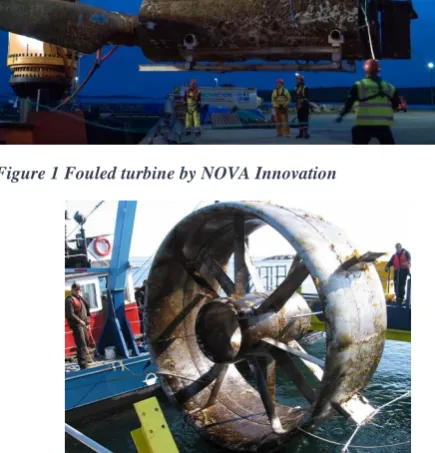
The power generating efficiency in HATT is mainly quantified by the power coefficient, 𝐶𝑃 which varies mainly with the conditions of the turbine. Therefore, understanding the behaviours of 𝐶𝑃 of a tidal turbine in real sea is particularly important to maintain the best performance of the HATT. However the NO.1 threat is the fouling caused by marine creatures, which has a profound impact on the levelized cost of energy, LCOE, due to its impact on the maintenance schedule of turbine blades. It can be seen first in the Figure 1, which demonstrates the marine fouling in the latest tidal turbine developed by NOVA Innovation. And the progress of fouling is develop on the tidal turbine blades with a staggering rate, which can been seen in Figure 2 taken by Clean Current Tidal Power Demonstration Project just after 6 months after the turbine has been deployed into the sea. Whereas tidal energy system is supposed to be able to operate for 20-25 years’ time. And it is now slowly getting the attention of the industrial leaders in the tidal energy industrial. However currently it is lack of clear solution. This is mainly because tidal energy technology is mainly inherited from the wind energy industrial, in terms of turbine design, manufacturing, drive train, control as well as power take off etc., in which marine fouling is never an issue for a wind turbine. However for tidal turbine it is the No.1 threat to its performance. In this context, it is of great importance understanding the effect of biofouling, which can occur almost everywhere in the sea.

Figure 1 Fouled turbine by NOVA Innovation

Figure 2 Fouling after 6 month (Clean Current Tidal Power Demonstration Project)

The accumulation of microorganisms, plants, algae, or animals on the surfaces of submerged, or semi-submerged, natural or artificial objects is termed marine biofouling (Lewis, 1998).

Thiobacilli, and/or other microorganisms quickly colonise any substrate placed in seawater (Gehrke and Sand, 2003). They form a sticky coating commonly referred to as a biofilm. The accumulation of biofilms not only brings the difficulties for subsea operators but also provide both a food source and a convenient interface to which the larger organisms, the macrofouling, can adhere (Titah-Benbouzid and (Titah-Benbouzid, 2015).

Fouling caused by large organisms, such as oysters, mussels, barnacles, seaweed and other organisms, is referred to as macrofouling. Macrofouling organisms can significantly affect the marine renewable energy convertors, by causing obstructions in the device and increasing the weight and drag. Accordingly, large economic costs follow due to the impaired equipment performance and the life span (Titah-Benbouzid and Benbouzid, 2015).

Fraenkel (2002) and Ng et al. (2013) identified the potential performance issues for marine turbines arising from the roughening of the turbine blades caused by the impact, cavitation or scour due to particulates, and the biofouling on the blade surface.

There have been few studies devoted to exploring the effect of surface roughness or fouling on marine turbines performances. Orme et al. (2001) investigated the potential effects of barnacles on the lift and drag coefficients for an aerofoil using a wind tunnel. The aerofoil was covered with idealised barnacles of different sizes and coverage densities, and they found decreased lift to drag ratio due to the idealised barnacles. Batten et al. (2008) studied the potential effects of increased blade roughness due to fouling using a numerical model based on blade element momentum (BEM) theory. They used larger drag coefficient 𝐶𝐷 in the numerical model for the fouled cases but the lift coefficient 𝐶𝐿 was not altered in the numerical model. The numerical model predicted 6-8% decrease in power coefficient 𝐶𝑃. Walker et al. (2014) conducted experimental and numerical studies to examine the effect of blade roughness and fouling on marine current turbine performance. They used a towing tank to test a model rotor in different surface conditions and a numerical BEM model was also developed altering the lift and drag coefficient according to the surface conditions. Both of their numerical and experimental results showed similar results suggesting that up to 19% of power coefficient 𝐶𝑃 can be reduced due to the surface roughness.

Although these studies clearly demonstrate the critical impact of biofouling on tidal turbine performances, they are still limited by several factors. First, it is questionable if the model-scale experiments can represent the hydrodynamic behaviour of full-scale tidal turbine. This is owing to the unique feature of the roughness effect in scaling. In other words, the size of surface roughness cannot be scaled proportionally to the model size, as argued by Franzini (1997). In terms of the numerical BEM models, the roughness effect on the blades were only considered as the altered lift and drag coefficients of the blades rather than solving the fluid field around the turbine, e.g. the pressure field around the blades, which can bring significant differences.

Implementation of computational fluid dynamics (CFD) is an effective way to overcome the above-mentioned difficulties. Eça and Hoekstra (2011) and Demirel et al. (2014) showed that CFD simulations using modified wall-function approach can precisely predict the roughness effects. In these CFD simulations the distribution of the local friction velocity, 𝑢𝜏, is dynamically computed for each discretized cell, and therefore the dynamically varying roughness Reynolds number, 𝑘+_{, and corresponding} roughness function, 𝛥𝑈+_{, can be taken into account in the} computation, and the roughness effect in the flow can be precisely predicted including the pressure field around the body. Recently, several studies used modified-wall function approaches in the CFD

models to investigate the roughness effect of biofouling on ship resistance (Demirel et al., 2017a; Song et al., 2019a) and marine propeller (Owen et al., 2018; Song et al., 2019b).

To the best of the authors’ knowledge, there exists no specific study to investigate the effect of biofouling on a full-scale tidal turbine using CFD. Therefore, the aim of this study is to fill this gap by developing a CFD model to simulate the effect of biofouling on the tidal turbine performances. The main advantage of the proposed approach is that the CFD model enables an extensive analysis on the hydrodynamic details of the turbulent flow over the rough surface of a full-scale tidal turbine in a fully non-linear way, which is not possible using experimental or theoretical methods.

In this study, a previously developed CFD approach was applied, for approximating the surface roughness due to barnacle fouling, in order to predict the effects on the HATT performances. Full-scale CFD simulations of the HATT in different fouling conditions were conducted at the tip speed ratios (TSR), ranging from 1 to 8. Finally, the impact of barnacle fouling on the power coefficients and thrust coefficients were examined.

2.

Numerical modelling

2.1. Roughness function

The surface roughness increases the turbulence. Accordingly, the turbulent stress, wall shear stress and finally the skin friction increases. The roughness effect can also be observed in the velocity profile in the log-law region. Clauser (1954) showed that the roughness effect results in a downward shift in the velocity profile in the log-law region. This downward shift is termed as the ‘Roughness Function’, 𝛥𝑈+_{. The non-dimensional velocity profile} in the log-law region for a rough surface is given as

𝑈+₌1

𝜅log 𝑦

+_{+ 𝐵 − 𝛥𝑈}+ ₍₁₎

The roughness function, 𝛥𝑈+ _{can be expressed as a function of the} roughness Reynolds number, 𝑘+_{, defined as}

𝑘+₌𝑘𝑈𝜏

𝜈

(2)

It should be borne in mind that 𝛥𝑈+_{simply vanishes in the case of a} smooth condition.

Demirel et al. (2017b) proposed an experimental approach to find the roughness functions of barnacle fouling. The study involves an extensive series of towing test of flat plates covered with artificial barnacle patches. Different sizes of real barnacles, categorised as small, medium and big regarding their size, were 3D scanned and printed into artificial barnacle tiles. The tiles then glued onto the flat plates by differing the coverage and the plates were towed at a range of speeds. Figure 3 shows the geometry of the 3D scanned barnacles and the barnacle patches glued on the plate.

From the analysis of the experimental results, they found that the roughness function behaviours of the barnacles follow the roughness function model of Grigson (1992) given as,

𝛥𝑈+₌1

𝜅ln(1 + 𝑘

+_{) (3)}

3 experimental result of Demirel et al (2017b) and showed an excellent agreement. In this study, the same modified wall-function approach as Song et al. (2019a) was used to simulate the surface roughness of barnacles of varying sizes and coverages.

Figure 3 Digitised barnacle geometry (left) and the flat plate covered with the barnacle patches (right), adapted from Demirel et al. (2017b)

Table 1 Roughness length scales of the fouling conditions, adapted from Demirel et al. (2017b)

Surface condition

Barnacle type

Surface coverage (%)

Barnacle height

ℎ (mm)

Representative sand-grain roughness height

𝑘_𝐺 (μm)

B10% Big 10 % 5 174

B20% Big 20 % 5 489

M10% Medium 10 % 2.5 84

M20% Medium 20 % 2.5 165

M40% Medium 40 % 2.5 388

M50% Medium 50 % 2.5 460

S10% Small 10 % 1.25 24

S20% Small 20 % 1.25 63

S40% Small 40 % 1.25 149

S50% Small 50 % 1.25 194

Figure 4 Roughness function for the fouling conditions, adapted from Demirel et al. (2017b)

2.2. Mathematical formulation

The proposed CFD model was developed based on the Reynolds-averaged Navier-Stokes (RANS) method using a commercial CFD software package, STAR-CCM+. The averaged continuity and momentum equations for incompressible flows may be given in tensor notation and Cartesian coordinates as in the following two equations (Ferziger and Peric, 2002).

𝜕(𝜌𝑢̅𝑖)

𝜕𝑥𝑖

= 0 (4)

𝜕(𝜌𝑢̅𝑖)

𝜕𝑡 +

𝜕 𝜕𝑥𝑗

(𝜌𝑢̅𝑖𝑢̅𝑗+ 𝜌𝑢̅̅̅̅̅̅) = −𝑖′𝑢𝑗′

𝜕𝑝̅ 𝜕𝑥𝑖

+𝜕𝜏̅𝑖𝑗 𝜕𝑥𝑗

(5)

in which, 𝜌 is density, 𝑢̅𝑖 is the averaged velocity vector, 𝜌𝑢̅̅̅̅̅̅𝑖′𝑢𝑗′ is the Reynolds stress, 𝑝̅ is the averaged pressure, 𝜏̅𝑖𝑗 is the mean viscous stress tensor components. This viscous stress for a Newtonian fluid can be expressed as

𝜏̅𝑖𝑗= 𝜇 (

𝜕𝑢̅𝑖

𝜕𝑥𝑗

+𝜕𝑢̅𝑗 𝜕𝑥𝑖

) (6)

where 𝜇 is the dynamic viscosity.

In the CFD solver, the computational domains were discretised and solved using a finite volume method. The second-order upwind convection scheme was used for the momentum equations. The flow equations were solved in a segregated manner. The continuity and momentum equations were linked with a predictor-corrector approach.

The shear stress transport (SST) 𝑘-𝜔 turbulence model was used to predict the effects of turbulence, which combines the advantages of the 𝑘-𝜔 and the 𝑘-ε turbulence model. This model uses a 𝑘-𝜔

formulation in the inner parts of the boundary layer and a 𝑘-ε

behaviour in the free-stream for a more accurate near wall treatment with less sensitivity of inlet turbulence properties, which brings a better prediction in adverse pressure gradients and separating flow (Menter, 1994). The volume of fluid (VOF) method was used for the models where free surfaces are present.

2.3. HATT geometry and simulation conditions

In this study, a full-scale CFD model of a typical three bladed HATT was developed. The turbine model was designed and tested by Wang et al. (2007) and validated by a model-scale CFD study (Shi et al., 2013). Table 2 and Figure 5 show the principal parameters and the geometry of the HATT.

The simulations were conducted in the smooth (clean) condition and 10 different fouling scenarios according to the barnacle sizes and coverages densities which can be found in Table 1. For each surface condition, simulations were conducted at the tip speed ratios, TSR, ranging 1-8. In order to vary the TSR values, the rotational speed (𝜔) was differed to match the corresponding TSR values, while the inlet velocity was remained constant (𝑉𝑖𝑛= 3.2𝑚/𝑠). The tip speed ratio, TSR was calculated as

TSR =𝜔𝑅

𝑉𝑖𝑛 (7)

where 𝜔, 𝑅, and 𝑉𝑖𝑛 are the rotational speed (rad/s), blade radius of the turbine (m) and the inlet velocity (m/s), respectively.

For each simulation case, the power coefficient, 𝐶𝑃, and thrust coefficients, 𝐶𝑇, were calculated as

𝐶𝑃=

𝑃 1 2𝜌𝐴𝑇𝑉𝑖𝑛3

(8)

𝐶𝑇=

𝑇 1 2𝜌𝐴𝑇𝑉𝑖𝑛2

(9)

where 𝑃 and 𝑇 are the power and the thrust of the turbine, 𝜌 and 𝐴𝑇 are the water density and the swept area of the turbine (𝜋𝑅2_), respectively.

Table 2 Main parameters of the HATT

Diameter (m) 20 Rotation rate (RPM) 12

Number of blades 3 Current speed (m/s) 3.2

Figure 5 Geometry of the HATT

2.4. Computational domain and boundary conditions

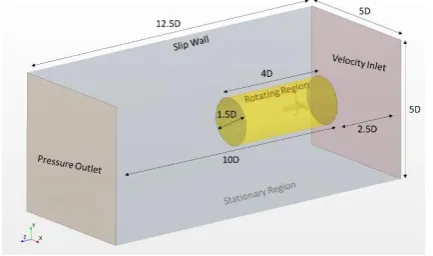
Figure 6 depicts an overview of the computational domain with the selected boundary conditions in the CFD simulations. The computational domain consists of a stationary region (outer zone) and a rotating region (inner zone). The inlet, outlet and surrounding walls were placed to simulate the conditions of the experiment conducted by Wang et al. (2007) using a cavitation tunnel.Me The boundary conditions for the inlet and outlet were defined as a velocity inlet and a pressure outlet, while the slip-wall boundary conditions were used for the surrounding walls, as the boundary layer flow on the wall is assumed to be negligible for the performance of the turbine.

The Moving Reference Frame (MRF) approach was used to simulate the rotating turbine (Luo et al., 1994). The MRF approach, also known as ‘Multiple Reference Frame’ or ‘Frozen Rotor Approach’, is a steady-state approximation in which individual cell zones can be assigned different translational and/or rotational motions and solved using the corresponding equations of the reference frames, e.g. the inner zone (yellow cylinder in Figure 6) using a rotating frame and the outer zone associated with a stationary frame in this study. Since the MRF approach does not require complicated mesh motion and uses a steady state solver for the flow field, it is simpler and computationally cheaper compared to other unsteady approaches (e.g. the Sliding Mesh). As proven by other studies (Mizzi et al, 2017; Owen et al, 2018; Song et al, 2019b), the authors believe that the MRF method does not bring any significant difference in the results compared to other unsteady methods, as this study is not concerning about the transient behaviours.

Figure 6 Domain and boundary conditions

2.5. Mesh generation

Mesh generation was performed using the built-in automated mesh tool of STAR-CCM+. Unstructured polyhedral meshes were used for simulation model, which enables to achieve accurate results with less computational cost. Local refinements were made for finer grids

in the critical regions, such as the region near the blades where the vortices and separations are expected to occur as shown in Figure 7. The prism layer meshes were used for near-wall refinement, and the thickness of the first layer cell on the surfaces was chosen such that the 𝑦+ _{value is always higher than 30 and 𝑘}+_{, as suggested by} Demirel et al. (2017a) and CD-Adapco (2017).

Figure 7 Grid system

3.

Results

3.1. Verification study

A verification study was carried out to evaluate the numerical uncertainties of the CFD model and to determine a sufficient mesh spacing. The Grid Convergence Index (GCI) method based on the extrapolation of Richardson (1910) was used to estimate the order of accuracy of the simulation model.

According to Celik et al. (2008) the apparent order of the method,

𝑝𝑎, is determined by

𝑝𝑎=

1 ln(𝑟21)| ln |

𝜀32

𝜀21| + 𝑞(𝑝𝑎

) | (10)

𝑞(𝑝𝑎) = ln (

𝑟₂₁𝑝𝑎_{− 𝑠}

𝑟₃₂𝑝𝑎_{− 𝑠}) (11)

𝑠 = 𝑠𝑖𝑔𝑛 (𝜀32

𝜀21) (12)

where 𝑟21 and 𝑟32 are refinement factors given by 𝑟21= √𝑁3 1/𝑁2 for a spatial convergence study of a 3D model. 𝑁 denotes the cell number of the numerical domain. 𝜀32=𝜙3− 𝜙2, 𝜀21=𝜙2− 𝜙1, and

𝜙𝑘 denote the key variables, e.g. 𝐶𝑃, or 𝐶𝑇 in this study. The extrapolated value is calculated by

𝜙𝑒𝑥𝑡21 =

𝑟₂₁𝑝𝜙1− 𝜙2

𝑟₂₁𝑝− 1 (13)

The approximate relative error, 𝑒𝑎21, and extrapolated relative error,

𝑒𝑒𝑥𝑡21, are then obtained by

𝑒𝑎21= |

𝜙1− 𝜙2

𝜙1 | (14)

𝑒𝑒𝑥𝑡21 = |

𝜙𝑒𝑥𝑡21 − 𝜙1

𝜙_𝑒𝑥𝑡21 | (15)

5

𝐺𝐶𝐼𝑓𝑖𝑛𝑒21 =

1.25𝑒𝑎21

𝑟₂₁𝑝 − 1 (16)

Three different grid resolutions were generated for the grid convergence study, which are referred to as fine, medium and coarse meshes corresponding total cell numbers of 𝑁1, 𝑁2, and 𝑁3. Table 3 indicates the required parameters for the numerical uncertainties arising from the spatial discretisation. The power coefficient, 𝐶𝑃 and thrust coefficient, 𝐶𝑇, at TSR=4, for the smooth case were used as the key variables. As shown in the table, the numerical uncertainties (GCI values) for 𝐶𝑃 and 𝐶𝑇 using the fine mesh are 0.24% and 0.04% respectively. For accurate prediction of the turbine performances, the fine mesh was used for the simulations.

Table 3 Discretisation error calculation for spatial convergence study

𝐶_𝑃 𝐶_𝑇

𝑁1 3,456,903 3,456,903

𝑁₂ 2,434,588 2,434,588

𝑁3 1,707,636 1,707,636

𝑟21 1.19 1.19

𝑟₃₂ 1.19 1.19

𝜙₁ (Fine) 4.551E-01 8.409E-01

𝜙2 (Medium) 4.529E-01 8.426E-01

𝜙3 (Course) 4.448E-01 8.319E-01

𝜀₃₂ -8.05E-03 -1.07E-02

𝜀21 -2.22E-03 1.63E-03

𝑠 1 -1

𝑒_𝑎21 _{4.88E-03 1.94E-03}

𝑞 -0.02 -0.02

𝑝_a 7.23 10.64

𝜙𝑒𝑥𝑡21 4.560E-01 8.407E-01

𝑒_𝑒𝑥𝑡21 _{-0.19% 0.04%}

𝐺𝐶𝐼_{𝑓𝑖𝑛𝑒}21

0.24% 0.04%

3.2. Validation study

Figure 8 and 9 compares the 𝐶𝑃 and 𝐶𝑇 obtained from the CFD model in smooth condition and the experimental data of Wang et al. (2007). To examine the scale effect together, the coefficients obtained from the simulations of model-scale turbine (D=0.4m) are also included in the figure. As presented in the figure, a good agreement was achieved between the CFD and EFD results, except for the overpredicted 𝐶𝑃 and 𝐶𝑇 values at high TSRs (6<TSR), and also overpredicted 𝐶𝑃 around TSR=2. Considering that the model-scale CFD results show good agreement with the EFD data, this difference can be most attributed to the scale effect due to the different Reynolds numbers. It is of note that the Reynold numbers, based on chord length at 0.7R and the relative flow velocity (𝑉𝑅=

√𝑉_𝐴2_{+ (0.7𝜔𝐷)}2_{) of the full-scale simulation and model-scale} experiment are 1.0 − 6.8 × 107 _{and 1.3 − 8.5 × 10}5_{, respectively.}

Figure 8 Comparison of the power coefficients obtained from the current CFD and EFD (Wang et al., 2007)

Figure 9 Comparison of the thrust coefficients obtained from the current CFD and EFD (Wang et al., 2007)

3.3. Roughness effect on the HATT

3.3.1.Power and thrust coefficient, 𝑪𝑷 and 𝑪𝑻

In order to investigate the impact of biofouling on the performance of the HATT, CFD simulations of the full-scale turbine were conducted in different fouling scenarios, shown in Table 1, at TSR ranging from 1 to 8.

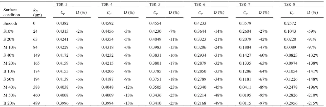
Figure 10 demonstrates the impact of the surface fouling on the power coefficients, 𝐶𝑃 of the turbine at each TSR. The fouling cases were sorted in the order of fouling severity, which can be represented by the representative sand-grain roughness height, 𝑘𝐺, in Table 1. As the table depicts, the 𝐶𝑃 values continuously decrease with increasing fouling rates. It was also noted that the reduction in 𝐶𝑃 becomes larger at higher TSR ranges. For example, the difference between the smooth and most severe fouling condition (B20%) is only 9% at TSR=3, and it increases to 213% at TSR=8, as can be seen in Table 4.

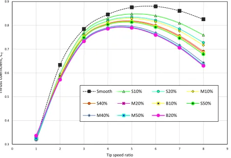
Figure 11 illustrates the power coefficients, 𝐶𝑃 of the different fouling scenarios versus the tip speed ratios, TSR. The increased power losses at higher TSRs are clearly seen in the figure. This rapid decreases in 𝐶𝑃 values at higher TSRs result in narrower operable TSR range. For instance, the TSR range where 𝐶𝑃 is higher than 0.4, for the most severe fouling condition (B20%), is 3.0 < TSR < 4.0 and it is narrower than a fifth of the that of smooth case, 2.25 < TSR < 7.4.

Another interesting finding from the result is the change in the optimum TSR point where the highest 𝐶𝑃 is found. Table 5 shows the maximum 𝐶𝑃 values for the different fouling scenarios and the corresponding TSR values. The roughness effect of the surface fouling not only reduces the maximum 𝐶𝑃 value of each case but also moves the corresponding rotational speed to lower TSR regions. It is of note that even for the mildest fouling case, the reduction of the optimum TSR is 14.2%. This finding suggests that the optimum TSR for the smooth condition is no longer valid once the surface is fouled and, hence, the surface condition should also be considered when the operating condition is planned, in order to achieve the maximum efficiency of tidal turbines.

Figure 11 compares the thrust coefficients, 𝐶𝑇 for the tidal turbine in the different fouling scenarios. Interestingly, it appeared that the surface roughness also decreases the 𝐶𝑇 values, which is desirable in terms of the survivability, apart from the drastic impact of biofouling on the 𝐶𝑃 values.

0 0.1 0.2 0.3 0.4 0.5 0.6 0.7

0 2 4 6 8 10

Po

w

er

co

ef

fi

ci

en

t,

CP

Tip speed ratio EFD

CFD (Model-scale) CFD (Full-scale)

0 0.2 0.4 0.6 0.8 1

0 2 4 6 8 10

Th

ru

st

c

o

ef

fi

ci

en

t,

CT

Tip speed ratio EFD

Figure 10 Comparisons of 𝑪𝑷 values in different fouling conditions at each TSR

Table 4 Comparisons of 𝑪𝑷 values in different fouling conditions

TSR=3 TSR=4 TSR=5 TSR=6 TSR=7 TSR=8

Surface condition

𝑘𝐺

(μm) 𝐶𝑃 D (%) 𝐶𝑃 D (%) 𝐶𝑃 D (%) 𝐶𝑃 D (%) 𝐶𝑃 D (%) 𝐶𝑃 D (%)

Smooth 0 0.4382 0.4592 0.4554 0.4233 0.3579 0.2572

S10% 24 0.4313 -2% 0.4456 -3% 0.4230 -7% 0.3644 -14% 0.2604 -27% 0.1043 -59%

S 20% 63 0.4241 -3% 0.4354 -5% 0.4049 -11% 0.3323 -21% 0.2079 -42% 0.0220 -91%

M 10% 84 0.4229 -3% 0.4318 -6% 0.3983 -13% 0.3206 -24% 0.1884 -47% 0.0089 -97%

S 40% 149 0.4172 -5% 0.4232 -8% 0.3831 -16% 0.2934 -31% 0.1427 -60% -0.0823 -132%

M 20% 165 0.4159 -5% 0.4215 -8% 0.3801 -17% 0.2879 -32% 0.1335 -63% -0.0974 -138%

B 10% 174 0.4153 -5% 0.4206 -8% 0.3785 -17% 0.2850 -33% 0.1286 -64% -0.1054 -141%

S 50% 194 0.4139 -6% 0.4187 -9% 0.3751 -18% 0.2789 -34% 0.1181 -67% -0.1226 -148%

M 40% 388 0.4038 -8% 0.4048 -12% 0.3505 -23% 0.2340 -45% 0.0411 -89% -0.2478 -196%

M 50% 460 0.4008 -9% 0.4009 -13% 0.3436 -25% 0.2214 -48% 0.0195 -95% -0.2826 -210%

B 20% 489 0.3996 -9% 0.3994 -13% 0.3410 -25% 0.2168 -49% 0.0115 -97% -0.2956 -215%

-15%

-21% -21% -22% -23% -23% -21%

-28% -24%

-19%

0.00 0.01 0.02 0.03 0.04 0.05 0.06

Smooth S10% S20% M10% S40% M20% B10% S50% M40% M50% B20% CP (TSR=1)

-9%

-20% -15% -18% -20% -21% -21% -24% -25% -25%

0.00 0.05 0.10 0.15 0.20 0.25 0.30 0.35 0.40

Smooth S10% S20% M10% S40% M20% B10% S50% M40% M50% B20% CP (TSR=2)

-2% -3% -3% -5% -5% -5% -6% _{-8% -9% -9%}

0.00 0.10 0.20 0.30 0.40 0.50

Smooth S10% S20% M10% S40% M20% B10% S50% M40% M50% B20%

CP (TSR=3)

-3% -5% -6% _{-8% -8% -8% -9%}

-12% -13% -13%

0.00 0.10 0.20 0.30 0.40 0.50

Smooth S10% S20% M10% S40% M20% B10% S50% M40% M50% B20%

CP (TSR=4)

-7% _-11%

-13% _{-16% -17% -17%}

-18%

-23% -25% -25%

0.00 0.10 0.20 0.30 0.40 0.50

Smooth S10% S20% M10% S40% M20% B10% S50% M40% M50% B20%

CP (TSR=5)

-14%

-21% _-24%

-31% -32% -33% -34%

-45% _{-48% -49%}

0.00 0.05 0.10 0.15 0.20 0.25 0.30 0.35 0.40 0.45

Smooth S10% S20% M10% S40% M20% B10% S50% M40% M50% B20%

CP (TSR=6)

-27%

-42% -47%

-60% _{-63% -64%}

-67%

-89%

-95% _-97%

0.00 0.05 0.10 0.15 0.20 0.25 0.30 0.35 0.40

Smooth S10% S20% M10% S40% M20% B10% S50% M40% M50% B20%

CP (TSR=7)

-59%

-91% _-97%

-132% -138% -141% _-148%

-196%

-210% -215% -0.40

-0.30 -0.20 -0.10 0.00 0.10 0.20 0.30

Smooth S10% S20% M10% S40% M20% B10% S50% M40% M50% B20%

7

Figure 11 Power coefficients calculated in different fouling scenarios

Table 5 Maximum 𝑪𝑷 value and corresponding TSR at each surface condition

Surface condition

𝑘𝐺 (μm) _{𝑂𝑝𝑡𝑖𝑚𝑢𝑚 𝐶}

𝑃 D (%) Corresponding TSR D (%)

Smooth 0 0.4604 0.4604 0.0%

S10% 24 0.4468 -3.0% 0.4468 -14.2%

S10% 63 0.4391 -4.6% 0.4391 -17.2%

M10% 84 0.4358 -5.3% 0.4358 -17.6%

S40% 149 0.4291 -6.8% 0.4291 -18.9%

M20% 165 0.4280 -7.0% 0.4280 -19.2%

B10% 174 0.4273 -7.2% 0.4273 -19.3%

S50% 194 0.4258 -7.5% 0.4258 -19.5%

M40% 388 0.4144 -10.0% 0.4144 -20.5%

M50% 460 0.4113 -10.7% 0.4113 -20.7%

B20% 489 0.4100 -10.9% 0.4100 -20.8%

-0.4 -0.3 -0.2 -0.1 0 0.1 0.2 0.3 0.4 0.5

0 1 2 3 4 5 6 7 8 9

Po

w

er

coef

fici

en

t,

CP

Tip speed ratio

Smooth S10% S20%

M10% S40% M20%

B10% S50% M40%

Figure 12 Thrust coefficients calculated in different fouling scenarios

3.3.2.Contribution of shear and pressure torque components

In order to investigate the rationale behind the increasing power loss due to the surface fouling at higher TSR regions, the components of the torque acting on the turbine were divided into shear and pressure components. Figure 13 illustrate the contributions of the pressure and shear components in the torque acting on the tidal turbine, in smooth condition and the most severe fouling (B20%) condition. As can be seen in the figure, the shear torques are acting on the negative direction of the turbine, and they increase with the TSRs. The fouled case has more than twice larger magnitudes of shear torques that those of smooth case over the TSR ranges. It can be deduced that the increased surface roughness due to the surface fouling results in increased skin friction and hence increases shear torque, which causes the efficiency loss.

Figure 13 also depicts that, for both surface conditions, the pressure components of torque decreases with TSRs, but the rate of decrease for the fouled case is much higher than that for the smooth case. This accelerated decrease can be seen as a cause of the rapid loss in, 𝐶𝑃, in conjunction with the increased shear torque due to the surface fouling.

Figure 13 Contribution of the torque coefficient components

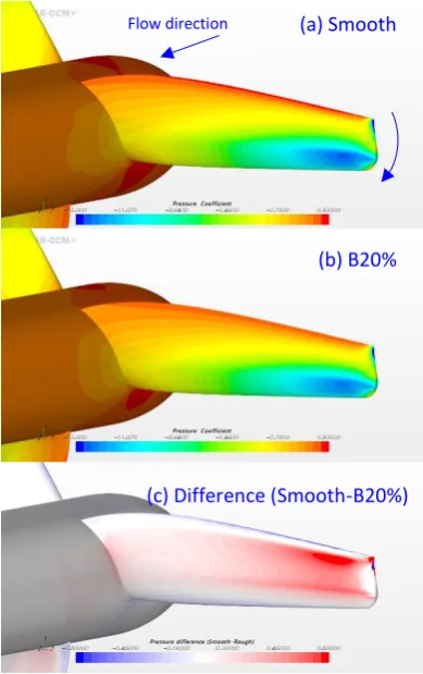
3.3.3.Surface pressure

Figure 14 and 15 compares the surface pressure on the turbine in the smooth and fouled (B20%) surface conditions. The pressure was nondimensionalised by dividing it by the dynamic pressure, 1/2𝜌𝑉2_. As can be seen in the figure, the fouled case has lower surface pressure on the blade in the face side and higher pressure in the back side. This observation is in agreement with the decreased pressure torque due to surface fouling, which can be found in Figure 13. 0.3

0.4 0.5 0.6 0.7 0.8 0.9

0 1 2 3 4 5 6 7 8 9

Th

ru

st

coef

fici

en

t,

CT

Tip speed ratio

Smooth S10% S20% M10%

S40% M20% B10% S50%

M40% M50% B20%

-1.0E+06 0.0E+00 1.0E+06 2.0E+06 3.0E+06 4.0E+06 5.0E+06

0 1 2 3 4 5 6 7 8 9

To

rque

(N

m

)

Tip Speed Ratio

9

Figure 14 Pressure distribution on the turbine surface at TSR=4 (face-side)

Figure 15 Pressure distribution on the turbine surface at TSR=4 (back-side)

3.3.1.Wall shear stress

Figure 16 illustrates the normalised wall shear stress magnitude on the turbine surface in the smooth and fouled (B20%) surface scenario at TSR=4. The wall shear stress was nondimensionalised by dividing it by the dynamic pressure, 1/2𝜌𝑉2_{. As can be seen in} the figure, significant increases in the wall shear stress were observed due to the surface fouling. The wall shear stress values for the fouled case were observed to be more than doubled due to the increased surface roughness, which is in accordance with the increased shear torque components observed in Figure 13.

Figure 16 Shear stress distribution on the turbine surface, at TSR=4

4.

Concluding remarks

A CFD model has been proposed for the investigation into the effect of biofouling on the performance of HATT. To represent the surface roughness of different fouling conditions, a previously-developed modified wall-function approach was used to approximate the roughness effects of barnacles of varying sizes and coverage densities.

A verification study was carried out to assess the numerical uncertainties of the proposed CFD model and to determine sufficient grid-spacings. The numerical uncertainties for 𝐶𝑃 and 𝐶𝑇 were estimated to be 0.24% and 0.04%, respectively.

As a validation study, 𝐶𝑃 and 𝐶𝑇 curves obtained from the CFD simulations were compared with the experimental data of Wang et al. (2007) and showed reasonable agreements.

Fully nonlinear RANS simulations of the full-scale HATT were performed in different fouling conditions at a range of tip speed ratios, to investigate the impact of barnacle fouling on the tidal turbine performance. The simulation results showed drastic impact of surface fouling on the efficiency of the tidal turbine. The power coefficients, 𝐶𝑃, showed decreasing trend with increasing fouling rates, and larger decreases were found at higher TSR regions. The decrease in the power coefficients, 𝐶𝑃 due to the surface fouling was found to be 9% at TSR=3, but it increased to 213% at TSR=8. This rapid reduction in 𝐶𝑃 appeared to cause narrower operable TSR ranges. In the most severe fouling condition (B20%), the operable TSR range (𝐶𝑃 > 0.4) was found to be narrower than a fifth of that for the smooth condition.

(a) Smooth

(b) B20%

(c) Difference (Smooth-B20%)

Flow direction

(a) Smooth

(b) B20%

(c) Difference (Smooth-B20%)

Flow direction

(a) Smooth

Another interesting finding from the result was that the optimum TSR point, where the highest 𝐶𝑃 is achieved, moved to lower TSR regions due to the surface fouling. This finding suggests that the optimum TSR for the smooth condition is no longer valid once the surface is fouled and the surface condition should be considered when the operating condition is planned, in order to achieve the maximum efficiency of tidal turbines.

The torque acting on the turbine were divided into the shear and pressure components, and it was found that the increased surface roughness due to the surface fouling causes in decreased torque and increased shear torque, resulting in reduced power coefficients. The surface pressure and wall shear stress were also examined, and reduced pressure difference between face and back side of the turbine and significantly increased wall shear stress were observed, which are in accordance with the reduced pressure torque and increased shear torque.

5.

Acknowledgements

It should be noted that the results were obtained using the ARCHIE-WeSt High Performance Computer (www.archie-west.ac.uk) based at the University of Strathclyde.

6.

References

Batten, W., Bahaj, A., Molland, A. F., & Chaplin, J. R. (2008). The Prediction of the Hydrodynamic Performance of Marine Current Turbines (Vol. 33).

CD-Adapco. (2017). STAR-CCM+ user guide, version 12.06. Celik, I. B., Ghia, U., Roache, P. J., Freitas, C. J., Coleman, H., &

Raad, P. E. (2008). Procedure for Estimation and Reporting of Uncertainty Due to Discretization in CFD Applications. Journal of Fluids Engineering, 130(7), 078001-078001-078004. doi: 10.1115/1.2960953 Charlier, R. H. (2003). A “sleeper” awakes: tidal current power.

Renewable and Sustainable Energy Reviews, 7(6), 515-529. doi: https://doi.org/10.1016/S1364-0321(03)00079-0 Clauser, F. H. (1954). Turbulent Boundary Layers in Adverse Pressure Gradients. Journal of the Aeronautical Sciences, 21(2), 91-108. doi: 10.2514/8.2938

Demirel, Y. K., Khorasanchi, M., Turan, O., Incecik, A., & Schultz, M. P. (2014). A CFD model for the frictional resistance prediction of antifouling coatings. Ocean Engineering, 89,

21-31. doi:

https://doi.org/10.1016/j.oceaneng.2014.07.017

Demirel, Y. K., Turan, O., & Incecik, A. (2017a). Predicting the effect of biofouling on ship resistance using CFD. Applied

Ocean Research, 62, 100-118. doi:

https://doi.org/10.1016/j.apor.2016.12.003

Demirel, Y. K., Uzun, D., Zhang, Y., Fang, H.-C., Day, A. H., & Turan, O. (2017b). Effect of barnacle fouling on ship resistance and powering. Biofouling, 33(10), 819-834. doi: 10.1080/08927014.2017.1373279

Eça, L., & Hoekstra, M. (2011). Numerical aspects of including wall roughness effects in the SST k–ω eddy-viscosity turbulence model. Computers & Fluids, 40(1), 299-314. doi: https://doi.org/10.1016/j.compfluid.2010.09.035 Ferziger, J. H., & Peric, M. (2002). Computational Methods for

Fluid Dynamics: Springer-Verlag Berlin Heidelberg. Fraenkel, P. L. (2002). Power from marine currents. Proceedings of

the Institution of Mechanical Engineers, Part A: Journal of Power and Energy, 216(1), 1-14. doi: 10.1243/095765002760024782

Franzini, J. (1997). Fluid Mechanics with Engineering Aplications: 9th edition (9 ed.). New York: McGraw-Hill.

Gehrke, T., & Sand, W. (2003). Interactions Between Microorganisms and Physiochemical Factors Cause MIC of Steel Pilings in Harbors (ALWC). Paper presented at the

CORROSION 2003, San Diego, California. https://doi.org/

Grigson, C. (1992). Drag losses of new ships caused by hull finish.

Journal of Ship Research, 36, 182-196.

Lewis, J. (1998). Marine biofouling and its prevention on underwater surfaces (Vol. 22).

Li, D., Wang, S., & Yuan, P. (2010). An overview of development of tidal current in China: Energy resource, conversion technology and opportunities. Renewable and Sustainable

Energy Reviews, 14(9), 2896-2905. doi:

https://doi.org/10.1016/j.rser.2010.06.001

Luo, J. Y., Issa, R. I., & Gosman, A. D. (1994). Prediction of impeller induced flows in mixing vessels using multiple frames of reference. Paper presented at the 8th European conference on mixing; INSTITUTION OF CHEMICAL ENGINEERS SYMPOSIUM SERIES, Cambridge. Menter, F. R. (1994). Two-Equation Eddy-Viscosity Turbulence

Models for Engineering Applications. AIAA Journal, 32(8), 1598-1605.

Mizzi, K., Demirel, Y. K., Banks, C., Turan, O., Kaklis, P., & Atlar, M. (2017). Design optimisation of Propeller Boss Cap Fins for enhanced propeller performance. Applied Ocean

Research, 62, 210-222. doi:

https://doi.org/10.1016/j.apor.2016.12.006

Ng, K.-W., Lam, W.-H., & Ng, K.-C. (2013). 2002–2012: 10 Years of Research Progress in Horizontal-Axis Marine Current Turbines. Energies, 6(3), 1497.

Orme, J. A. C., Masters, I., & Griffiths, R. T. (2001). Investigation of the effect of biofouling on the efficiency of the marine current turbines. Paper presented at the the Marine Renewable Energy Conference, Newcastle Upon Tyne, UK.

Owen, D., Demirel, Y. K., Oguz, E., Tezdogan, T., & Incecik, A. (2018). Investigating the effect of biofouling on propeller characteristics using CFD. Ocean Engineering. doi: https://doi.org/10.1016/j.oceaneng.2018.01.087

Pelc, R., & Fujita, R. M. (2002). Rnewable enrgy from the ocean.

Marine Policy, 26, 471-479.

Richardson, L. F. (1910). The approximate arithmetical solution by finite differences of physical problems involving differential equations, with an application to the stresses in a masonry dam. Transcations of the Royal Society of London. Series A, 210, 307-357.

Shi, W., Wang, D., Atlar, M., & Seo, K. C. (2013). Flow separation impacts on the hydrodynamic performance analysis of a marine current turbine using CFD. Proceedings of the Institution of Mechanical Engineers, Part A: Journal of Power and Energy, 227(8), 833-846. doi: 10.1177/0957650913499749

Song, S., Demirel, Y. K., & Atlar, M. (2019b). An investigation into the effect of biofouling on full-scale propeller performance using CFD. Paper presented at the OMAE, Glasgow.

Song, S., Demirel, Y. K., & Mehmet, A. (2019a). An Investigation into the Effect of Biofouling on the Ship Hydrodynamic Characteristics using CFD. Ocean Engineering.

Titah-Benbouzid, H., & Benbouzid, M. (2015, 2015-09-06). Marine Renewable Energy Converters and Biofouling: A Review on Impacts and Prevention. Paper presented at the EWTEC 2015, Nantes, France.

Walker, J., Flack, K., Lust, E., Schultz, M., & Luznik, L. (2014).

Experimental and numerical studies of blade roughness and fouling on marine current turbine performance (Vol. 66).