City, University of London Institutional Repository
Citation
:
Kao, C., Trapani, L. and Urga, G. (2018). Testing for instability in covariance
structures. Bernoulli : official journal of the Bernoulli Society for Mathematical Statistics and
Probability, 24(1), pp. 740-771. doi: 10.3150/16-BEJ894
This is the published version of the paper.
This version of the publication may differ from the final published
version.
Permanent repository link: http://openaccess.city.ac.uk/15475/
Link to published version
:
http://dx.doi.org/10.3150/16-BEJ894
Copyright and reuse:
City Research Online aims to make research
outputs of City, University of London available to a wider audience.
Copyright and Moral Rights remain with the author(s) and/or copyright
holders. URLs from City Research Online may be freely distributed and
linked to.
DOI:10.3150/16-BEJ894
Testing for instability in covariance structures
C H I H WA K AO1, L O R E N Z O T R A PA N I2and G I OVA N N I U R G A3
1Center for Policy Research, 426 Eggers Hall, Syracuse University, Syracuse, NY 13244-1020 (USA).
E-mail:[email protected]
2Centre for Econometric Analysis, Faculty of Finance, Cass Business School, 106 Bunhill Row, London
EC1Y 8TZ (UK). E-mail:[email protected]
3Centre for Econometric Analysis, Faculty of Finance, Cass Business School, 106 Bunhill Row, London
EC1Y 8TZ (UK) and Bergamo University (Italy). E-mail:[email protected]
We propose a test for the stability over time of the covariance matrix of multivariate time series. The analysis is extended to the eigensystem to ascertain changes due to instability in the eigenvalues and/or eigenvectors. Using strong Invariance Principles and Law of Large Numbers, we normalise the CUSUM-type statistics to calculate their supremum over the whole sample. The power properties of the test versus alternative hypotheses, including also the case of breaks close to the beginning/end of sample are investi-gated theoretically and via simulation. We extend our theory to test for the stability of the covariance matrix of a multivariate regression model. The testing procedures are illustrated by studying the stability of the principal components of the term structure of 18 US interest rates.
Keywords:changepoint; covariance matrix; CUSUM statistic; eigensystem
1. Introduction
In this paper, we propose a testing procedure to evaluate the structural stability of the covariance matrix (and its eigensystem) of multivariate time series. A large amount of empirical evidence shows that the issue of changepoint detection in a covariance matrix is of great importance. A classical example is the application of Principal Component Analysis (PCA) to the term struc-ture of interest rates, with the three main principal components interpreted as “slope”, “level” and “curvature” [28]. Bliss [7], Bliss and Smith [8] and Perignon and Villa [31] show that the prin-cipal components of the term structure change substantially over time. Similar findings, using a different methodology, are in [4]. PCA is also widely used in macroeconometrics, for instance to forecast inflation [34–36]. The importance of verifying the stability of a covariance matrix is also evident in the context of Vector AutoRegressive (VAR) models. In the context of forecast-ing, [9] show that changes in the smallest eigenvalue of the covariance matrix of the error term have a large impact on predictive ability. Furthermore, the Choleski decomposition of the error covariance matrix is routinely employed in the context of variance decomposition analysis, when examining how much of the variance of the forecast error of each variable in a VAR is due to exogenous shocks to the other variables (see, e.g., [32]).
Despite the relevance of the topic, most studies either assume stability as a working assump-tion without testing for it, or the testing is carried out by splitting the sample, thus assuming knowledge of the break date a priori. This calls for a rigorous testing procedure to estimate the location of the changepoint when breaks are detected.
The theoretical framework developed in this paper builds on a plethora of results for the changepoint problem available in statistics and in econometrics. Existing testing procedures (see, e.g., the reviews by [6,12]; and [24]) are typically based on taking the supremum (or some other metric – see [3]) of a sequence of CUSUM-type statistics, thus not requiring prior knowledge of the breakdate. In particular, [5] develop a test for the structural stability of a covariance ma-trix, based on minimal assumptions. However, a feature of this test is that, by construction, it has power versus breaks occurring at least (respectively, at most)O(√T )time periods from the beginning (respectively, to the end) of the sample. Lack of power versus alternatives close to ei-ther end of the sample is a typical feature in this literature (see also [2]), which somewhat limits the applicability of the test. Situations where breaks are due to recent events, like for example, the 2008 recession, are left out of the analysis. Our contribution complements that of [5] by proposing a test that has power versus breaks occurring close to the beginning/end of the sample. The main contribution of this paper is twofold. First, testing for changepoints is extended to PCA. In addition, the extension to testing for the stability of principal components is useful for the purpose of dimension reduction. Our simulations show that tests for the stability of the whole covariance matrix have severe size distortions in finite samples. Contrary to this, testing for the stability of eigenvalues is found to have the correct size and good power even for relatively small samples. As a second contribution, our testing procedure is able to detect breaks occurring up toO(ln lnT ) periods to the end of the sample. This is achieved by using a Strong Invariance Principle (SIP) and a Strong Law of Large Numbers (SLLN) for the partial sample estimators of the covariance matrix, and by using these results to normalize the CUSUM-type test statistic, using a Darling–Erd˝os limit theory (see [12,22]). In the Supplemental Material to this paper (henceforth referred to as [25]), we also extend our results to the case of testing for the stability of the covariance matrix of the error term in a multivariate regression setting.
The theory derived in our paper is illustrated through an application to the US term structure of interest rates, with a dataset spanning from the late nineties to the current date. We find (as expected) evidence of changes in the volatility and in the loading of the principal components of the term structure around the end of 2007/beginning of 2008. In the Supplemental Material [25], we also report another exercise, based on verifying the stability of the covariance matrix of the error term in a VAR model for exchange rates.
The paper is organized as follows. Section2contains the SIP and its extension to the eigen-system. The test statistic and its distribution under the null (as well as its behaviour under local-to-null alternatives) is in Section3. Monte Carlo evidence is in Section4, while the application to the term structure of interest rates is in Section5. Section6concludes.
A word on notation. Limits are denoted as “→” (the ordinary limit); “→p” (convergence in probability); “→d” and (convergence in distribution). Orders of magnitude for an almost surely convergent sequence (saysT) are denoted asOa.s.(Tς)andoa.s.(Tς)when, for someε >0 and
˜
T <∞,P[|T−ςsT|< εfor allT ≥ ˜T] =1 andT−ςsT →0 almost surely, respectively. Orders
of magnitude for a sequence converging in probability (say sT) are denoted as Op(Tς) and
op(Tς)when, for someε >0,ε>0 andT˜ε<∞,P[|T−ςsT|> ε]< εfor allT >T˜ε and
T−ςsT →0 in probability, respectively. Standard Wiener processes and Brownian bridges of dimensionqare denoted asWq(·)andBq(·), respectively;vdenotes the Euclidean norm of a
Lp-norm; the integer part of a real numberxis denoted asx . Constants that do not depend on
the sample size are denoted asM,M,M, etc.
2. Theoretical framework
This section derives results on the convergence rate of the sample covariance matrix, its eigen-system, and an estimator of its asymptotic variance, assuming a covariance stationary time series with no breaks. These calculations are useful in Section3, for deriving the null distribution of our test.
Let{yt}Tt=1be a time series of dimensionn; we assume thatyt has zero mean and covariance
matrix≡E(ytyt). This section contains the asymptotics of the partial sample estimates of;
the results are used in Section3in order to construct the CUSUM-type test statistic to test for breaks inand its eigensystem. Specifically, we report a SIP for the partial sample estimators of and an estimator of the long run covariance matrix of the estimated, sayV; and we extend
the asymptotics to PCA.
Strong invariance principle and estimation of
V
Let be the sample covariance matrix, i.e. =T−1Tt=1ytyt. For a given τ ∈ [0,1], we
define a point in time T τ , and we use the subscripts τ and 1−τ to denote quantities cal-culated using the subsamples t=1, . . . ,T τ andt = T τ +1, . . . , T, respectively. In par-ticular, we consider the sequence of partial sample estimators τ =(T τ )−1tT τ=1 ytyt, and
similarly1−τ = [T (1−τ )]−1Tt=T τ +1ytyt. Finally, henceforth we denotewt=vec(ytyt)
andw¯t =vec(ytyt−).
In the sequel, we need the following assumption.
Assumption 1. (i) suptEyt2r<∞for somer >2; (ii)ytisL2+-NED (Near Epoch
Depen-dent) for some >0, of sizeα∈(1,+∞)on an i.i.d. basis{vt}+∞t=−∞, withr >2αα−−11(1+
2);
(iii) letting V,T =T−1E[(
T t=1w¯t)(
T
t=1w¯t)], V,T is positive definite uniformly in T,
and as T → ∞, V,T → V with V <∞; (iv) letting w¯it be the ith element of w¯t
and definingSiT ,m≡
m+T
t=m+1w¯it, there exists a positive definite matrix ¯ = {ij}such that
T−1|E[SiT ,mSj T ,m] −ij| ≤MT−ψ, for alliandj and uniformly inm, withψ >0.
Assumption1specifies the moment conditions and the memory allowed inyt; no distributional
assumptions are required. According to part (i), at least the 4th moment ofyt is required to be
finite, similarly to [5]. As far as serial dependence is concerned, the requirement thatytbe NED
is typical in nonlinear time series analysis (see [17]) and it implies thatyt is a mixingale [13].
Many of the DGPs considered in the literature generate NED series – examples include GARCH, bilinear and threshold models (see [14]). Part (ii) illustrates the trade-off between the memory of yt(i.e., its NED sizeα), and its largest existing moment: asα(the memory ofyt) approaches 1,
(viz., they are squared), and therefore the relationship between moment conditions and memory is not the “standard” one (see, e.g., the IP in Theorem 29.6 in [13]). In principle, moment conditions such as the one in part (ii) could be tested for, for example, using a test based on some tail-index estimator – Hill [19,20] extends the well-known Hill’s estimator to the context of dependent data. Other types of dependence could be considered, for example, assuming a linear process foryt
– an IP for the sample variance is in [33], Theorem 3.8. Part (iv) is a bound on the growth rate of the variance of partial sums ofw¯t, and it is the same as Assumption A.3 in [11]. Although
it is not needed to prove the IP for the partial sum process ofw¯t, it is a sufficient condition for
the SIP; despite it being rather technical, it can be shown to hold for example, for the case of a weakly stationary sequence (see Proposition 2.1 in [16]).
Theorem1contains the IP and the SIP for the partial sums ofw¯t.
Theorem 1. Under Assumptions1(i)–(iii),asT → ∞
1
√
T T τ
t=1
¯
wt d
→ [V]1/2Wn2(τ ), (1)
uniformly inτ.Redefiningw¯t in a richer probability space,under Assumptions1(i)–(iv),there
exists aδ >0such that
T τ
t=1
¯
wt=
T τ
t=1
Xt+Oa.s.
T τ 12−δ, (2)
uniformly inτ,whereXt is a zero mean,i.i.d.Gaussian sequence withE(XtXt)=V.
Remarks. T1.1 Equation (1) is an IP forw¯t(i.e. a weak convergence result), which is sufficient
to use the test statistics discussed for example, in [2] and [3].
T1.2 Equation (2) is an almost sure result, which also provides a rate of convergence. The practical consequence of (2) is that the dependent, heteroskedastic seriesw¯t can be replaced with
a sequence of i.i.d. normally distributed random variables, with the same long run variance as
¯
wt. In both results – (1) and (2) – one difference with the literature is that we are dealing with
a non-Lipschitz transformation of NED data (essentially,w¯t is the square ofyt), which requires
some intermediate results on the dependence inw¯t itself; we refer to the Supplemental Material
[25] for the whole set of derivations.
We now turn to the estimation ofV. If no serial dependence is present, a possible choice is
the full sample estimatorV=T1Tt=1wtwt− [vec() ][vec()]. Alternatively, one could use
the sequence of partial sample estimators
V,τ=
1 T
T
t=1
wtwt−
τvec(τ) vec(τ)+(1−τ )
vec(1−τ) vec(1−τ)
To accommodate for the casel≡E(w¯tw¯t−l)=0 for somel, we propose a weighted
sum-of-covariance estimator with bandwidthm:
˜
V=0+
m
l=1
1− l m
l+l , (3)
wherel=T1Tt=l+1[wt−vec()][wt−l−vec() ]; orV˜,τ=(0,τ+0,1−τ)+ml=1(1−
l
m)[(l,τ + l,τ )+ (l,1−τ +l,1−τ)], where l,τ =
1
T
T τ
t=l+1[wt − vec(τ)][wt−l −
vec(τ)], and similarly forl,1−τ.
In order to derive the asymptotics ofV,τ andV˜,τ, consider the following assumption:
Assumption 2. (i) Either (a) l =0 for all l =0 or (b)
∞
l=0lsl<∞ for s =1;
(ii) suptEyt4r<∞for somer >2; (iii) letting T =T−1E{
T
t=1vec[ ¯wtw¯t−E(w¯tw¯t)] ×
vec[ ¯wtw¯t−E(w¯tw¯t)]}, T is positive definite uniformly inT, and T → with <∞.
Assumption2encompasses various possible cases. Part (i)(a) considers the basic, non autocor-related case, for which bothV andV,τ are valid choices. Part (i)(b) considers the possibility
of non-zero autocorrelations. Intuitively, the assumption that the 4th moment ofyt exists, as in
Assumption1(i), entails, through a Law of Large Numbers (LLN), the consistency ofV,τ. Part
(ii) supersedes Assumption1(i), by requiring the existence of moments up to the 8th. Intuitively, this implies that an IP holds for the partial sums of vec[ ¯wtw¯t−E(w¯tw¯t)].
The consistency ofV,τ and ofV˜,τ is in Theorem2:
Theorem 2. Under no changes in:
if Assumptions1(i)–(iii)and2(i)(a)hold,asT → ∞,there exists aδ>0such that
sup
1≤T τ ≤T
V,τ−V =op
1 Tδ
; (4)
if Assumptions1(i)–(iii)and2(i)(b)hold,as(m, T )→ ∞,there exists aδ>0such that
sup
1≤T τ ≤T
˜V,τ−V =Op
1 m
+Op
mlnT Tδ
; (5)
if Assumptions1(i)–(iii)and2(i)(b)–(ii)–(iii)hold,as(m, T )→ ∞
sup
1≤T τ ≤T
˜V,τ−V =Op
1 m
+Op
mln√T T
. (6)
The same rates hold forVorV˜.
Remarks. T2.1 Equation (4) is based on a SLLN for the case of no autocorrelation inwt – see
required in this literature (e.g., Lemma 2.1.2 in [12], page 76; see also the proof of Theorem3
below). In case of serial dependence, (5) states that it is possible to construct an estimator ofV
with a rate of convergence. This can be refined as in (6).
T2.2 A word of warning on the weighted-sum-of-covariance estimatorV˜,τ is in order. As
well-documented in several contributions (we refer to [30], and the references therein, for an exposition of the issues),V˜,τ can be expected to suffer from (possibly severe) finite sample bias,
especially in the presence of large autoregressive roots. In Section4, we assess the robustness of
˜
V,τ to the case of strong serial correlation in the data.
Estimation of the eigensystem
In this section, we extend the asymptotics for the partial sample estimates ofto its eigensystem. Let theith eigenvalue/eigenvector couple be defined as(λi, xi); the eigenvectors are defined
as an orthonormal basis, that is,xixj=δij, whereδij is Kronecker’s delta. Sincexi =λixi,
a natural estimator for(λi, xi)is the solution to the system
X=X,
XX=I, (7)
whereX= [ ˆx1, . . . ,xˆn],xˆidenotes the estimate ofxi, andis a diagonal matrix containing the
estimated eigenvaluesλˆi in decreasing order. Estimation of{(λi, xi)}ni=1based on (7) is known
as Anderson’s Principal Component (PC) estimator. Similarly, the partial sample estimators of the eigenvalues and eigenvectors are the solutions toτxˆi,τ= ˆλi,τxˆi,τ.
As we mention below (see Remark P1.2), one disadvantage of Anderson’s PC estimator is that the estimated eigenvectors have a singular asymptotic covariance matrix (see [26]). In order to avoid this issue, an estimator based on a different normalisation can be proposed, known as the Pearson–Hotelling’s PC estimator; in this case, the estimated eigenvalues are the same as from (7), but the eigenvectorsγiare defined (and estimated) as an eigenvalue-normed basis, viz.
γiγj =λiδij. Thus,γi ≡λ1i/2xi. A typical interpretation of theγis in the context of the term
structure of interest rates [28,31] is thatλiis the “volatility” ofγi, andxirepresents its “loading”.
The estimates of the eigensystem according to the Pearson–Hotelling approach are the solution to the system
X=X,
XX=. (8)
Upon calculating the solutions of (8), it turns out that the eigenvectors are estimated byγˆi =
ˆ
λ1i/2xˆi, that is, by the same estimator for the eigenvector as in (7) multiplied by the square root
of the corresponding estimate of the eigenvalue. Similarly, we define the partial sample estimator ofγi asγˆi,τ = ˆλ
1/2
i,τxˆi,τ.
Consider the following assumption.
Assumption 3requires that has distinct, strictly positive eigenvalues, and it is typical of PCA, affording to use Matrix Perturbation Theory (MPT); the assumption could be relaxed at the price of a more complicated analysis, still based on MPT. In essence, the asymptotics of (λˆi,τ,xˆi,τ)is derived by treatingτas a perturbation of, thus deriving the expressions for the
estimation errors ofλˆi,τ andxˆi,τ. The way in which the assumption is formulated is the same
as in [23], see equation (1.11). As a consequence of the requirement that eigenvalues be strictly positive, our set-up does not directly cover the case of exact factor models, where the covariance matrix of the data has reduced rank by construction – see [18,37] and [10].
The extension of the IP and the SIP to the eigensystem ofis reported in Proposition1:
Proposition 1. Under Assumptions1and3,asT → ∞,uniformly inτ
ˆ
λi,τ−λi=
xi⊗xivec(τ−)+Op
T−1, (9)
ˆ
xi,τ −xi=vx,ivec(τ−)+Op
T−1, (10)
ˆ
γi,τ −γi=vγ ,ivec(τ−)+Op
T−1, (11)
wherevx,i= [k=i xk
λi−λk(x
k⊗xi)]andvγ ,i=
1 2
xi
λ1i/2(x
i⊗xi)+
k=i λ1i/2xk
λi−λk(x
i⊗xk).
Remarks. P1.1 Proposition1 is the central ingredient in order to apply the test for structural breaks to the eigensystem. It states that the estimation errorsλˆi,τ −λi,xˆi,τ −xi andγˆi,τ−γi
are, asymptotically, linear functions of τ −; thus, the IP and the SIP in Theorem1 carry
through to the estimated eigensystem. The results in Proposition1, and the method of proof, can be compared to related results in [26].
P1.2 By (10), the asymptotic covariance matrix of √T (xˆi,τ −xi) is vx,iVvx,i. It can be
shown (see, e.g., [26], page 66) thatvx,iVvx,i is singular; given that there is no obvious way
to calculate the rank ofvx,iVvx,i , it is difficult to prove the consistency of the Moore–Penrose
inverse forvx,iVvx,i (see [1]). Thus, we recommend to carry out tests on the eigenvectors using
theγi’s.
P1.3 Proposition 1 shows that λˆi,τ −λi is linear in τ − to the order Op(T−1); the
proof of the proposition shows that the leading order term in the approximation error is T−1k=i[ ˆxi⊗ ˆxk] V˜
ˆ
λi−ˆλk[ ˆ
xk⊗ ˆxi], so finite sample improvements may be obtained usingλ˜i,τ=
ˆ
λi,τ−T−1
k=i[ ˆxi⊗ ˆxk]
˜
V
ˆ
λi−ˆλk[ ˆ
xk⊗ ˆxi]. This result is of independent interest; it could be useful
e.g. when measuring the percentage of the total variance ofyt explained by each of its principal
components. Similarly, in equation (36) inAppendixwe provide a formula to estimate the ex-pected value of theOp(T−1)order terms of(xˆi,τ−xi); combining these results, a bias-correction
forγˆi,τ can also be computed.
Define λ≡ [λ1, . . . , λn] as the n-dimensional vector containing the eigenvalues sorted in
Op(T−1)andDλγ ≡ [x1⊗x1, . . . , xn⊗xn, vγ , 1, . . . , vγ ,n ]. The matrixDλγ can be estimated as
Dλγ= [ ˆx1⊗ ˆx1, . . . ,xˆn⊗ ˆxn,vˆγ , 1, . . . ,vˆγ ,n], withvˆγ ,i=12ˆxˆi λ1i/2(xˆ
i⊗ ˆxi)+
k=i
ˆ
λ1i/2xˆk
ˆ
λi−ˆλk
(xˆi⊗ ˆxk). The asymptotics ofzˆτ follows from Theorem1and Proposition1, and we summarize it below.
Corollary 1. Under Assumptions1 and3,asT → ∞,it holds that√T (zˆτ−z) d
→ [Vz]1/2×
Wn(2n+1)(τ ). Also, there exists a δ >0 such that T (zˆτ −z)=t=T τ1 X˜t +Oa.s.(T τ
1 2−δ), uniformly inτ,whereVz=DλγVDλγ and X˜t is a zero mean,i.i.d.Gaussian sequence with
E(X˜tX˜t)=Vz.
Corollary1entails that
√
T (λˆτ−λ) d
→ [Vλ]1/2Wn(τ ),
√
Tvec(τ−) d
→ [V]1/2Wn2(τ ),
with:Vλ a matrix with (i, j )th element given by Vijλ=(xi⊗xi)V(xj ⊗xj), and V is an
(n2×n2)-dimensional matrix whose(i, j )thn×nblock is defined asVij=vγ ,iVvγ ,j.
3. Testing
This section studies the null distribution and the consistency of tests based on CUSUM-type statistics.
Henceforth, we define the CUSUM processS(τ )=t=T τ1 vec(ytyt). In light of Corollary1,
test statistics forand its eigensystem can be based on
˜
S(τ )=R×Dλγ×
S(τ )−T τ T S(1)
, (12)
withS(τ )˜ =0 forτ≤ T1 or≥1−T1, andRap×n(n+1)matrix. For example, when testing for the null of no changes in the largest eigenvalue,Ris the matrix that extracts the first element ofDλγ× [S(τ )−T τT S(1)]. Thence, testing is carried out by using (the supremum of)
T(τ )=
T
T τ × T (1−τ ) ×
˜
S(τ )V˜z,τ−1S(τ )˜ 1/2, (13)
withV˜z,τ =RDλγV˜,τDλγR. The test statistic defined in (13) can be compared with the one
proposed by [5], which, in our context, would be based on (the supremum of)
AT(τ )=
1 T ×
˜
Contrasting (13) with (14), it is clear that the only difference between the two test statistics is
the norming factors,
T
T τ ×T (1−τ ) versus
1
T. However, such difference is crucial: by virtue
of the weighing scheme proposed in (13), we are able to detect the presence of breaks closer to either end of the sample than afforded by (14). More specific comments on the power properties of tests based on (13) versus tests based on (14) are in the remarks to Theorem4; here we point out that the price to pay is that we are not able to study the limiting distribution of the supremum of (13) using the IP shown in Theorem1, but conversely the SIP is needed.
Theorem3contains the asymptotics of supT τ T(τ )under the null.
Theorem 3. Under Assumptions1–3,as(m, T )→ ∞with m1 +mln√T
T →0,
sup T τ1 ≤T τ ≤T τ2
T(τ ) d
→ sup
τ1≤τ≤τ2
Bp(τ )
√
τ (1−τ ), (15)
where Bp(τ ) is a p-dimensional standard Brownian bridge and [τ1, τ2] ⊂(0,1). Also, as
(m, T )→ ∞with √
ln lnT
m +mlnT
ln lnT T →0,
P
aT
sup
n≤T τ ≤T−n
T(τ )
≤x+bT
→e−2e−x, (16)
whereaT =
√
2 ln lnT andbT =2 ln lnT+p2ln ln lnT−ln(p2),with(·)the Gamma function.
Remarks. T3.1 According to (15), the maximum is taken in a subset of[0,1], namely[τ1, τ2].
This approach requires an IP forS(τ ), and the Continuous Mapping Theorem (CMT). As noted in Corollary 1 in [2], page 838,T(τ )is not continuous at{0,1}and sup1≤T τ ≤T T(τ )
p
→ ∞
under H0. Thus, trimming is necessary in this case. Further, in this case it suffices to have a
consistent estimator of the long-run covariance matrix V which, in light of equation (6) in
Theorem2, entails thatm→ ∞withm=o(T ). The considerations in Remark T2.1 apply here. T3.2 As an alternative approach, the SIP can be used: sums ofw¯t can be replaced by sums
of i.i.d. Gaussian variables, with an approximation error. Upon normalisingT(τ )with the
ap-propriate norming constants, sayaT andbT, an Extreme Value (EV henceforth) theorem can
be employed. Tests based on supn≤T τ ≤T−n[aTT(τ )−bT]are designed to be able to detect
breaks close to the end of the sample. Results like (16) have been derived by [22], for i.i.d. Gaussian data, and extended to the case of dependence by [27],inter alia. As far as the long-run covariance matrix estimator is concerned, in this case the theory requires a consistent estimator at a rate (at least)op[(
√
ln lnT )−1]: therefore, from (6), we need the restrictions √
ln lnT
m →0 and
mlnT
Consistency of the test
We now turn to studying the behaviour of supn≤T τ ≤T−nT(τ )under alternatives. As a leading
example, we consider the case of testing for no change inin presence of one abrupt change
Ha(T ):vech(t)=
vech(), fort=1, . . . , k0,T,
vech()+T, fort=k0,T +1, . . . , T ,
(17)
where both the changepoint (k0,T) and the size of the break (T) could depend onT. More
general alternatives could be considered (see, e.g., [2,12]): these include epidemic alternatives, and also breaks that occur as a smooth transition over time as opposed to abruptly as in (17). Further, note that (17) does not rule out the possibility that only some series (i.e. only some of the coordinates ofyt) actually have a break. This entails that tests based onT(τ )are capable
of detecting breaks that only affect some of the series, and possibly at different points in time. Theorem4illustrates the dependence of the power onT andk0,T.
Theorem 4. Let Assumptions1–3hold,and definecα,T such that,underH0,
P
sup
n≤T τ ≤T−n
T(τ )≤cα,T
=1−α
for someα∈ [0,1].If,underHa(T ),asT → ∞
1 ln lnT
(T−k0,T)k0,T
T RDλγT
2
→ ∞, (18)
it holds that
P
sup
n≤T τ ≤T−n
T(τ ) > cα,T
→1. (19)
Remarks. T4.1 Theorem4illustrates the impact ofk0,T andT on the power of tests based on
supn≤T τ ≤T−nT(τ ). Particularly, consider the two extreme cases:
T4.1.aT =O(1), that is, finite break size. In this case, the test has power as long ask0,T
is strictly bigger thanO(ln lnT ). This can be compared with tests based on sup1≤T τ ≤TT−1×
˜
S(τ )V˜z,τ−1S(τ )˜ , which can be shown to have nontrivial power in presence of finite breaks at most as close asO(√T ) to either end of the sample. Using similar algebra as in the proof of Theorem4, it can be shown that the noncentrality parameter of sup1≤T τ ≤TT−1S(τ )˜ V˜z,τ−1S(τ )˜
is proportional toT2 k2
0,T
T . UnderT =O(1), this entails that nontrivial power is attained
as long ask0,T =O(
√
T ).
T4.1.bk0,T =O(T )– that is, the break occurs in the middle of the sample. The test is powerful
as long as the size of the break is strictly bigger thanO(
ln lnT
T ). When using trimmed statistics
such as in (15), the test is powerful versus mid-sample alternatives of sizeO(√1
T): when no
T4.2 Equation (18) also indicates that the test has no power whenRDλγT =0 (or whenever
it is “very small”). This could for example happen in the case of having a break, however massive, in the eigenvalueλi, and applying the test for a change in eigenvalueλj,j =i; such a test is
bound to have no ability to detect a change inλi, by construction.
In the Supplemental Material [25], we also show that all the results developed above also hold when applied to residuals – that is, one can test for the stability of the covariance matrix (and its eigensystem) of the error term in the multivariate regression (including e.g., a VAR)
yt=βxt+εt, (20)
wheret =1, . . . , T andyt andεt aren×1 vectors,xt is of dimensionq×1 (and results can
be extended to also include linear or polynomial trends inxt) and the matrix of regressorsβhas
dimensionsn×q. As shown in the Supplemental Material [25], the extension to residuals only requires thatxtεt andεt satisfy similar assumptions to the one spelt out above.
Computation of critical values
Based on Theorem3, there are two possible approaches to the computation of critical values: either using the EV distribution in (16) or using an approximation similar to that proposed in [12], Section 1.3.2.
Direct computation of critical valuescα,T for a test of levelαis based oncα,T =aT−1{bT −
ln[−12ln(1−α)]}. Thus, critical values only depend onpandT. It is well known that conver-gence to the EV distribution is usually very slow, which hampers the quality of cα,T.
Alterna-tively, critical values can be simulated from
P
sup
hnT≤τ≤1−hnT
p
i=1
B12,i(τ ) τ (1−τ )
1/2
≤cα,T
=1−α, (21)
where theB1,i(τ )s are independent, univariate Brownian bridges, generated over a grid of
di-mensionT. We setT ×hnT =max{n,ln3/2T}. The “time series” part of this bound (i.e., the
ln3/2T part) is based on [12], page 25, who show that computing the maxima over restricted intervals (specifically, by truncating atT×hnT =ln3/2T) yields tests with good size properties;
4. Monte Carlo evidence
We evaluate size and power through a Monte Carlo exercise. Data are generated according to the following DGP:
yt=ρyt−1+et+θ et−1. (22)
Under the null, we simulate et as i.i.d. N (0, In). Our experiments are conducted by setting
(ρ, θ )= {(0,0), (0.5,0), (0,0.5), (0,−0.5)}; as far as the sample sizeT, and the matrix dimen-sionn, are concerned, experiments are reported forT = {50,200,500}andn= {3,10}. Finally, in order to avoid dependence on initial conditions,T +1000 data are generated, discarding the first 1000 observations.
As far as the test is concerned, this is based on
sup
T hnT≤T τ ≤T−T hnT
T(τ ), (23)
wherehnT is defined above ashnT =max{Tn,ln
3/2T
T }. In all experiments, we use the long run
variance estimator in (3), based on full sample estimation of the autocovariance matrices with m=T2/5.
Testing for changes in the largest eigenvalue
In the first set of experiments, we test for the null of no changes in the largest eigenvalue of. Under the alternative, breaks inE(etet)are defined as
In, fort=1, . . . , k,
In+, fort=k+1, . . . , T .
(24)
Breaks are evaluated according to the following schemes
k=
T 2
and =
ln lnT
T2/3 ×In, (25)
k=
T 2
and =
ln lnT
T1/2 ×In, (26)
k=T hnT +1, k=
1 2(lnT )
2, k=1
2(lnT )
5/2
and k=3√T;=In. (27)
The first two alternatives consider power versus mid-sample breaks; the last set of alternatives considers breaks of finite magnitude that are close to the beginning of the sample.
We note that:
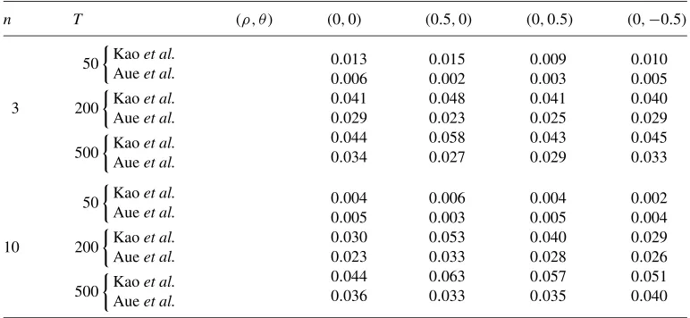
Table 1. Empirical rejection frequencies for the null of no changes in the largest eigenvalue of. Data are generated according to equation (22)
n T (ρ, θ ) (0,0) (0.5,0) (0,0.5) (0,−0.5)
3
50
Kaoet al.
Aueet al.
200
Kaoet al.
Aueet al.
500
Kaoet al.
Aueet al.
0.013 0.006 0.041 0.029 0.044 0.034
0.015 0.002 0.048 0.023 0.058 0.027
0.009 0.003 0.041 0.025 0.043 0.029
0.010 0.005 0.040 0.029 0.045 0.033
10
50
Kaoet al.
Aueet al.
200
Kaoet al.
Aueet al.
500
Kaoet al.
Aueet al.
0.004 0.005 0.030 0.023 0.044 0.036
0.006 0.003 0.053 0.033 0.063 0.033
0.004 0.005 0.040 0.028 0.057 0.035
0.002 0.004 0.029 0.026 0.051 0.040
frequencies belonging, in general, to the interval[0.04,0.06]with few exceptions. Interest-ingly, higher values ofnhave a slight tendency to reduce the size. Similar results are found with [5] test based on (14);
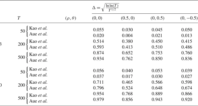
2. As far aspoweris concerned:
(a) mid-sample breaks are studied in Tables2–3, which correspond to cases (25) and (26), respectively. The test has good power, with the power increasing asnincreases. As predicted by the theory, the test by [5] has higher power. Note the adverse impact of higher serial correlation on both tests;
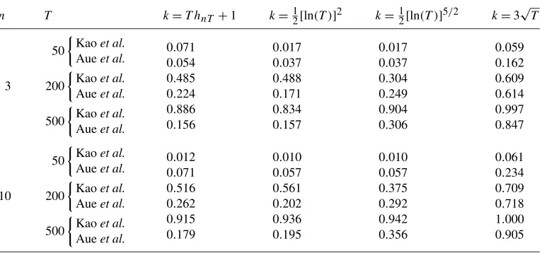
(b) breaks close to the beginning of the sample are considered in Table4, corresponding to equation (27). The test has power versus finite alternatives that are close to the beginning of the sample, and the power increases withn;
– as is natural, [5] test has very little power versus beginning of sample alternatives; by construction, such tests do not have power versus changes that occur closer thanO(√T ) periods to the beginning (or the end) of the sample; again, note the adverse effect of higher serial correlation on the power of both tests.
Testing for changes in the covariance matrix
We also carry out a second set of experiments to evaluate the performance of the test when applied to detect a change in E(ytyt). The test is based on the null that all eigenvalues are
Table 2. Power of the test for the null of no changes in the largest eigenvalue of. Data are generated according to equation (22) and under the alternative hypothesis specified in equation (25)
=
ln ln(T ) T2/3
n T (ρ, θ ) (0,0) (0.5,0) (0,0.5) (0,−0.5)
3
50
Kaoet al.
Aueet al.
200
Kaoet al.
Aueet al.
500
Kaoet al.
Aueet al.
0.035 0.014 0.235 0.293 0.427 0.533
0.021 0.001 0.180 0.185 0.302 0.350
0.027 0.010 0.211 0.228 0.371 0.424
0.034 0.006 0.191 0.232 0.335 0.410
10
50
Kaoet al.
Aueet al.
200
Kaoet al.
Aueet al.
500
Kaoet al.
Aueet al.
0.032 0.020 0.356 0.440 0.528 0.661
0.026 0.012 0.247 0.248 0.364 0.430
0.033 0.021 0.273 0.328 0.449 0.536
0.021 0.015 0.309 0.336 0.434 0.537
Table 3. Power of the test for the null of no changes in the largest eigenvalue of. Data are generated according to equation (22) and under the alternative hypothesis specified in equation (26)
=
ln ln(T ) T1/2
n T (ρ, θ ) (0,0) (0.5,0) (0,0.5) (0,−0.5)
3
50
Kaoet al.
Aueet al.
200
Kaoet al.
Aueet al.
500
Kaoet al.
Aueet al.
0.055 0.020 0.514 0.593 0.874 0.934
0.030 0.004 0.380 0.413 0.652 0.762
0.045 0.021 0.450 0.510 0.753 0.850
0.050 0.013 0.415 0.486 0.760 0.836
10
50
Kaoet al.
Aueet al.
200
Kaoet al.
Aueet al.
500
Kaoet al.
Aueet al.
0.056 0.037 0.711 0.796 0.954 0.979
0.040 0.017 0.465 0.524 0.768 0.856
0.053 0.030 0.566 0.648 0.889 0.943
[image:15.488.46.423.373.575.2]Table 4. Power of the test for the null of no changes in the largest eigenvalue of. Data are generated as i.i.d., under the alternative specified in equation (27)
n T k=T hnT +1 k=12[ln(T )]2 k=12[ln(T )]5/2 k=3
√ T
3
50
Kaoet al.
Aueet al.
200
Kaoet al.
Aueet al.
500
Kaoet al.
Aueet al.
0.071 0.054 0.485 0.224 0.886 0.156
0.017 0.037 0.488 0.171 0.834 0.157
0.017 0.037 0.304 0.249 0.904 0.306
0.059 0.162 0.609 0.614 0.997 0.847
10
50
Kaoet al.
Aueet al.
200
Kaoet al.
Aueet al.
500
Kaoet al.
Aueet al.
0.012 0.071 0.516 0.262 0.915 0.179
0.010 0.057 0.561 0.202 0.936 0.195
0.010 0.057 0.375 0.292 0.942 0.356
0.061 0.234 0.709 0.718 1.000 0.905
The main findings are as follows:
1. As far assizeis concerned, asnincreases, the test becomes increasingly conservative in finite samples; however, asT → ∞, the empirical rejection frequencies tend towards their nominal values;
2. As far aspoweris concerned:
(a) under mid-sample alternatives, the power increases monotonically with T as ex-pected. As far asnis concerned, the power seems to have a mild tendency to increase with n. As expected, in this context our test is less powerful than the one proposed by [5], and it has power higher than 50% whenT ≥200;
(b) under end-of-sample alternatives, asnincreases, the power also increases. As ex-pected, our test is decidedly more powerful than the test by [5], at least for large samples (T ≥200). Neither test has satisfactory power when the sample size is small;
(c) in both experiments, we also considered a break of equal magnitude and location as above, but only for the first element in the matrix, that is, the volatility of the first series. We considered the case of i.i.d. data only. Results are comparable with the rest of the tables.
Other experiments
1. The case of anearly singular covariance matrix(Table B1 in the Supplementary Material) has been simulated by usinget∼N (0, Cn)in the DGP defined in equation (22), whereCnis an
n-dimensional diagonal matrix defined as
{Cn}ii=
1, fori=1,
U[0,0.02], for 2≤i≤n. (28)
This set-up, with one large eigenvalues and the others being very small, corresponds to the case of having a factor model. By way of comparison, we also carried out the same exercise, but with data generated by settinget∼N (0, In). We test for the stability of the first principal component,
considering size and power versus mid-sample and end-of-sample alternatives: in presence of very small eigenvalues, the test still has good size and power properties, although power is better (especially asngrows) when eigenvalues are of comparable magnitude.
2. The case ofhighly autocorrelated data(Table B2 in the Supplementary Material) has been simulated using the following variant of the DGP defined in (22)
yt=0.9yt−1+et. (29)
Without pre-whitening, the test is so grossly oversized (empirical rejection frequencies, under the null, are well above 50%) that we do not even report the results: the basic message is that the test cannot be employed in presence of highly correlated data. This is essentially due to the poor performance of the long-run variance estimator; unreported experiments where the test is carried out using the population long-run variance reinforce this conjecture. As a solution, we suggest pre-whitening, which in our case we carry out by estimating a VAR(1)and using a short bandwidth chosen asm=T1/4: in this case, results are very good in terms of power and size. By way of robustness check, we have also tried to assess whether, in presence of a mis-specified pre-whitening, the test works well – to this end, we have simulated data as
yt=0.9yt−1+et+0.9et−1,
with pre-whitening being carried out as before – that is, by using a VAR(1). Results show that even when pre-whitening is not correctly specified, the test has the correct size, and good power versus mid-sample alternatives; however, the power versus breaks close to either end of the sam-ple is significantly lower when the pre-whitening is not correctly specified.1
5. Application: The time stability of the covariance matrix of
interest rates
In this section, we apply the theory developed above to test for the stability of the covariance matrix of the term structure of interest rates – returns, computed as log differences of zero-coupon
bond prices are used, since preliminary analysis shows that the yields are highly persistent. Our analysis is motivated by the study in [31], and follows similar steps.
As a first step, we investigate whether the “volatility curve”(i.e., the term structure of the volatility of interest rates) changes over time; this corresponds to testing for the stability of the main diagonal of the covariance matrix. Further, we verify whether the whole covariance matrix changes. This could be done by directly testing for the constancy of the matrix. Alternatively, in order to reduce the dimensionality of the problem, one could check whether the main three prin-cipal components (customarily known as level, slope and curvature) are stable through time. We choose the latter approach, verifying separately, for each principal component, whether sources of time variation are in the loadings (i.e., the eigenvectors) or in the volatility (i.e., the eigenval-ues), or both.
Previous studies have found evidence of changes in the yield curve. Using a descriptive ap-proach based on splitting the sample at some predetermined points in time, indicated by stylised facts, [7] finds that the eigenvectors of the covariance matrix of interest rates are quite stable, al-though the eigenvalues differ across subsamples. Perignon and Villa [31], under the assumption that data are i.i.d. Gaussian, find evidence of changes in the volatilities (eigenvalues) of the prin-cipal components across four different subperiods (chosena priori) in the time interval January 1960–December 1999.
We apply our test to US data, considering monthly and weekly frequencies, spanning from April 1997 to November 2010 (monthly – the sample size isTm=164) and from the first week
of April 1997 to the last week of November 2010 (weekly – the sample size isTw=713); the use
of different frequencies within the same endpoint may be helpful to show whether the properties of the data depend on their frequency or not. The number of maturities which we consider is n=18, corresponding to (1m, 3m, 6m, 9m, 12m, 15m, 18m, 21m, 24m, 30m, 3y, 4y, 5y, 6y, 7y, 8y,9y,10y). Figure1reports the term structure in the period considered.
In the Supplemental Material, we also report some descriptive statistics (Table C). Since there seems to be some serial correlation (at least with lower maturities), we pre-whiten the data using the VAR(1) scheme employed in the previous section. We letytdenote, henceforth, the demeaned
18-dimensional vector of maturities. The first step of our analysis is an evaluation of the stability of the variances, that is, of the elements on the main diagonal of=E(ytyt). Instead of
check-ing for the stability of the whole main diagonal, we test the volatilities one by one; this approach should be more constructive if the null of no changes were to be rejected, in that it would indicate which maturity changes and when. In order to control for the size of this multiple comparison, we propose a Bonferroni correction, computing the critical values for each test asαI=αnP, where
αP is the size of the whole procedure. Using these critical values yields, approximately, a level
αP not greater than 1%, 5% and 10% corresponds to conducting each test at levelsαI=0.056%,
0.28% and 0.56%, respectively.
As a second step, we verify whether the first three principal components are constant over time. Particularly, we carry out separately the detection of changes in the volatility of the principal components (verifying the time stability of the three largest eigenvalues, sayλ1,λ2andλ3), and
in their loading (verifying the stability of the eigenvalue-normed eigenvectors corresponding to the three largest eigenvalues, denoted asγ1,γ2 andγ3). As far as eigenvectors are concerned,
(10) and (11) ensure that, when running the test, the CUSUM transformation of the estimatedγis
Figure 1. Term structure of the US interest rates. Maturities correspond to 1m,3m,6m,9m,12m,15m,
18m,21m,24m,30m,3y,4y,5y,6y,7y,8y,9y,10yover the period April 1997–November 2010.
Results for both experiments, at both frequencies, are reported in Table5(critical values are in Table D in the Supplemental Material [25]).
Interestingly, when using a 5% level, rejections occur for the same maturities, whether one uses the Bonferroni correction or not. The only exception is the test for the stability of the second eigenvector,γ2, when using weekly data, where the null of no change is now rejected at 5%.
A marginal discrepancy can be observed in Panel A of Table5, when testing for the constancy of the diagonal elements of with weekly data. When considering a single hypothesis testing approach, two maturities (the 30 months and the 3 years ones) now appear to have a break. The rest of the results (especially the absence of breaks in monthly data) is the same as when using a Bonferroni correction.
Table5shows some discrepancy between monthly and weekly data. Monthly data, as a whole, have a stabler covariance structure over time, with no changes in the volatilities of the maturities, or in any of the principal components. Indeed, the only instability is observed in the eigenvalue structure (Panel B):λ3, the volatility of the curvature, has a break significant at 5%. The
C.
Kao,
L.
T
rapani
and
G.
Ur
[image:20.488.111.643.116.432.2]ga
Table 5. Tests for changes in the variances of the term structure; in the volatilities of each principal component; and in the eigenvalue-normed eigenvectors. Rejection at 10%, 5% and 1% levels are denoted with∗,∗∗and∗∗∗respectively. Where present, numbers in square brackets are the estimated breakdates, defined asT×arg maxT(τ )
Panel A Panel B Panel C
H0:iiconstant H0:λiconstant H0:γi constant
i Monthly Weekly Monthly Weekly Monthly Weekly
1m 2.6989 2.8421 λ1 1.6921 3.5798∗∗ x1 3.9142 6.957∗∗
3m 2.7656 3.5461 [1st week, 12/2007] [3rd week, 03/2008]
6m 2.7394 3.0854 λ2 2.5513 2.7488 x2 4.3898 7.098∗∗
9m 2.3924 2.1531 [3rd week, 04/2008]
12m 1.5350 2.9454 λ3 3.4328∗∗ 2.7726 x3 4.2340 7.261∗∗∗
15m 1.4991 2.6190 [01/2008] [2nd week, 03/2008]
18m 1.6467 2.4979 21m 1.8065 2.6907 24m 1.9827 2.9462 30m 2.0718 3.1947 3y 2.0815 3.4064 4y 1.9314 3.7837 5y 1.8964 3.8836∗
[1st week, 12/2007] 6y 1.8369 4.0432∗∗
[1st week, 12/2007] 7y 1.7677 4.0488∗∗
[1st week, 12/2007] 8y 1.9601 4.1446∗∗
[1st week, 12/2007] 9y 2.1046 4.2285∗∗
[last week, 08/2008] 10y 2.1967 4.3417∗∗
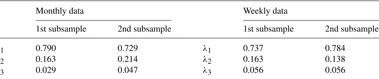
Table 6. Proportion of the total variance explained by principal components (λ1,λ2andλ3refer to the level, slope and curvature respectively) for each subsample. The samples are split based on the results in Table2. When considering monthly data, the sample was split at January 2008; when using weekly data, at the first week of December 2007
Monthly data Weekly data
1st subsample 2nd subsample 1st subsample 2nd subsample
λ1 0.790 0.729 λ1 0.737 0.784
λ2 0.163 0.214 λ2 0.163 0.138
λ3 0.029 0.047 λ3 0.056 0.056
are subject to change: the level and the curvature change significantly around the middle/end of March 2008 (possibly due to an “attraction” effect of the variance of the 10-year maturity); the slope has a significant break also, a few weeks later. The presence of significant changes in the loadings of each principal component as a result of the 2007–2009 recession is a different feature to what [31] found in the time period they consider, when eigenvectors were not subject to changes over time.
Finally, we report the proportion of the total variance explained by each principal component before and after this date.
6. Conclusions
In this paper, we propose a test for the null of no breaks in the eigensystem of a covariance ma-trix. The assumptions under which we derive our results are sufficiently general to accommodate for a wide variety of datasets. We show that our test is powerful versus alternatives as close to the boundaries of the sample asO(ln lnT ). Results are extended to testing for the stability of the eigensystem. We also derive a correction for the finite sample bias when estimating eigenvalues and eigenvectors, which can be relatively severe for largenor smallT. The theory is also ex-tended to develop tests for the null of no change in the covariance matrix of the error term in a multivariate regression (including the case of VARs; see the Supplemental Material [25]. As shown in Section4, the properties of the test are satisfactory: the correct size is attained under various degrees of serial dependence, and the test exhibits good power.
The results in this paper suggest several avenues for research. An important issue is the spec-ification of the long-run variance estimator when implementing the test. Monte Carlo evidence suggests that employing the estimator with pre-whitening, subsequently choosing a small band-width, yields good results – this could be an initial guideline for the applied user. Also, the theory is derived under the minimal assumption that the 4th moment exists. Aueet al.[5] provide a dis-cussion as to how to proceed if this is not the case, which involves fractional transformations of the series, viz.yitfor some∈(0,1), although the optimal choice ofis not straightforward. Also, the estimator of the long-run varianceVproves to be crucial in affecting the properties of
Appendix: Proofs of the main results
Proof of Theorem1. The proof of (1) is essentially based on checking the validity of the as-sumptions in Theorem 29.6 in [13], page 481, for the normalized sequence w¯T ,t=V,T−1/2w¯t.
In light of Lemma 2 in the Supplemental Material [25], w¯T ,t, for given values of α and r
in Assumption 2, is L2-NED on the strong mixing base {vt}+∞t=−∞ with size α> 12, which
entails the validity of Assumption (c) in [13]; Theorem 29.6. Assumption 1(ii) implies that E(w¯T ,t)=V,T−1/2E(w¯t)=0. Assumption (b) in Theorem 29.6 in [13], page 482, follows from
Assumption1(ii) and from noting that, in light of Assumption1(i), suptE( ¯wtr/2) <∞.
As-sumptions (d) and (f) in Theorem 29.6 in [13] are implied by Assumption1(iii). Finally, As-sumption (e) follows from the LLN entailed by AsAs-sumptions1(iii). Thus, (1) holds.
As far as (2) is concerned, its proof is based on Theorem 1 in [16], page 263. Lemma 2 in the Supplemental Material [25] entails thatw¯t is a zero-meanL2+-mixingale of sizeα>
1
2. Letting m= { ¯w1,...,w¯m} andST m≡
m+T
t=m+1w¯t, (2) follows if |E[ST m|m]|2<∞ and
|E[SiT mSj T m|m] −E[SiT mSj T m]| =O(T1−θ)forθ >0 and alli,j. Both conditions can be
proved following the same passages as in [11], pages 651–652.
Proof of Theorem2. The proof is similar to the proof of Lemma 2.1.1 in [12], pages 74–75. In view of Lemma 3 in the Supplemental Material [25], a SLLN holds (see [27], Theorem 2.1), whereby for alll
1
T τ T τ
t=1
vecw¯tw¯t−l−E
¯
wtw¯t−l =oa.s.
1
T τ δ
;
similarly,τ −=oa.s.(T τ −δ
), sincewt also satisfies the assumptions needed for
Theo-rem 2.1 in [27]. This entails that, for anyε >0 andε>0, there is an integergT =gT(ε, ε)such
that
P
sup
gT≤T τ ≤T
T τ δl,τ−l> ε
≤ε,
P
sup
1≤T τ ≤T−gT
T τ δl,τ−l> ε
≤ε.
These yield sup1≤T τ ≤T l,τ −l =op( 1
Tδ). This proves (4).
In order to prove (5), note that
˜V,τ−V ≤
(0,τ−τ 0)+0,1−τ−(1−τ )0
+2
m
l=1
1− l m
(l,τ−τ l)+l,1−τ−(1−τ )l
+2
m
l=1
l
ml +2 ∞
l=m+1
l
=I+II+III.
Note first that Assumption2(i)(b) entailsIII=o(m−s); clearly, this holds uniformly inτ. Also, again by Assumption2(i)(b),II=2m−1O(1)=O(m−1), again uniformly inτ. We now study I; in particular, we will consider the quantityml=0(1− ml)(l,τ −τ l). Letting wˆ¯t =wt −
vec(τ), we have
E m
l=0
1− l m
1 T
T τ
t=1
ˆ¯
wtwˆ¯t−l−l
2
≤T−2
m
l=0
m
h=0
E
T τ
t=1
ˆ¯
wtwˆ¯t−l−l
T τ
t=1
ˆ¯
wtwˆ¯t−h−h
≤T−2
m
l=0
m
h=0
E1/2
T τ
t=1
ˆ¯
wtwˆ¯t−l−l
2
E1/2
T τ
t=1
ˆ¯
wtwˆ¯t−h−h
2
;
we know by the proof of Theorem 2.1 in [27] that there is a constant δ >0 such that E1/2t=T τ1 (wˆ¯twˆ¯t−l−l)2=O(T τ 1−δ); therefore,
E m
l=0
1− l m
1 T
T τ
t=1
ˆ¯
wtwˆ¯t−l−l
2
=Om2T τ −2δ,
which entails (see [29])
E sup
0≤m≤m
sup
1≤T τ ≤T
m
l=0
1− l m
1 T
T τ
t=1
ˆ¯
wtwˆ¯t−l−l
2
=Om2T−2δlnmlnT,
and note that lnm≤lnT. Hence, it can be shown that
sup
1≤T τ ≤T
(0,τ−τ 0)+0,1−τ−(1−τ )0
+2
m
l=1
1− l m
(l,τ−τ l)+l,1−τ−(1−τ )l
=Op