City, University of London Institutional Repository
Citation
:
Kyriazis, N., Koukouvinis, F. ORCID: 0000-0002-3945-3707, Karathanassis, I. K. ORCID: 0000-0001-9025-2866 and Gavaises, M. ORCID: 0000-0003-0874-8534 (2018). A tabulated data technique for cryogenic two-phase flows. Paper presented at the 7thEuropean Conference on Computational Fluid Dynamics, 11-15 Jun 2018, Glasgow, UK.
This is the accepted version of the paper.
This version of the publication may differ from the final published
version.
Permanent repository link:
http://openaccess.city.ac.uk/20507/Link to published version
:
Copyright and reuse:
City Research Online aims to make research
outputs of City, University of London available to a wider audience.
Copyright and Moral Rights remain with the author(s) and/or copyright
holders. URLs from City Research Online may be freely distributed and
linked to.
A TABULATED DATA TECHNIQUE FOR CRYOGENIC TWO-PHASE
FLOWS
NIKOLAOS KYRIAZIS, PHOEVOS KOUKOUVINIS, IOANNIS KARATHANASSIS AND MANOLIS GAVAISES
City, University of London EC1V 0HB
[email protected] [email protected] [email protected]
Key words:Cryogenic flows, LOX simulation, Helmholtz Equation of state.
Abstract. Flashing flows of liquid oxygen (LOX) are prevalent in space applications, where LOX can be used as rocket engine propellant [1]–[3]. Towards this direction, the cryogenic flow in a converging-diverging nozzle has been investigated in the present study by utilising real fluid thermodynamics under the homogeneous equilibrium mixture (HEM) assumption for the LOX. A tabulated data method for the Helmholtz energy equation of state (EoS) has been developed in OpenFOAM (OF) [4] and has been incorporated into an explicit density based solver. Due to the wide variation of the speed of sound and consequently of the Mach number noticed in the liquid, vapour and mixture phases, a Mach consistent numerical flux has been employed suitable for subsonic up to supersonic flow conditions [5]. Since the Helmholtz EoS is computationally inefficient compared to simplified EoS, an ad-hoc thermodynamic table containing all the thermodynamic properties for the LOX has been created and stored prior entering the time loop [6], accompanied by a static linked-list algorithm for reducing the search time. Once the thermodynamic element of the table which satisfies the values of the density and internal energy as predicted from the numerical solution of the Navier-Stokes equations is identified, the unknown thermodynamic properties are approximated by a finite element interpolation [7]. The numerical method has been firstly validated against the Riemann problem at similar cryogenic flow conditions. Then, 2-D axisymmetric simulations of the phase-change process in a converging-diverging nozzle are performed and compared with prediction from other numerical tools as well as experimental data. It is concluded that the results are satisfactory while the applicability of the Helmholtz EoS to LOX simulations is demonstrated. This suggests that the proposed methodology can be utilized for the simulation of flashing flows.
1 INTRODUCTION
compared to other fuels in such applications. Aiming to minimize the fuel tank structure in the rocket, oxygen is stored in liquid form (LOX). For instance, LOX is used in the Ariane 5 and in the future Arianne 5ME upper stage engines [9]. Complex thermodynamic modelling is therefore required for such cryogenic flow applications. Experimental studies are scarce due to the cryogenic flow conditions [10]–[12], which pose questions about the accuracy and reliability of the results [9], while there is also little information in the literature regarding LOX simulations, which necessitate real fluid thermodynamics to be employed; see for example [13], [14].
For modelling cryogenic flows, either two-fluid or one-fluid models have been employed in numerous past studies. The two-fluid model, which was originally introduced by Wallis in 1980 [15], considers slip velocity and non-equilibrium effects. However, such models strongly depend on closure models describing the interaction between the two phases, thus rendering the relevant methodologies problem dependent. Maksic and Mewes [16] simulated flashing in converging-diverging nozzles by employing a transport equation for the bubble number density (4-equation model) to the continuity, momentum and energy equations. Later on, a 6-equation model (continuity, momentum and enthalpy equations for each phase separately) has been used by Marsh, O’ Mahony [17] for flashing flows and by Mimouni [18] for boiling flows, where Janet et al. [19] utilised a 7-equation model and they considered nucleation during flashing flow in converging-diverging nozzles. In the latter, a bubble number transport equation was added in the system of 6 equations.
On the other hand, in one-fluid models the same velocity, pressure and temperature fields are assumed, since the phases are assumed to be in thermal and mechanical equilibrium. The Homogeneous Relaxation Model (HRM), which considers non-equilibrium vapour generation, was introduced by Bilicki and Kestin [20]; later on, Schmidt et al. [21] expanded HRM to 2-D problems. In another mixture approach, Travis et al. [14] utilised the Helmholtz EoS for isentropic cryogenic flows of hydrogen, methane, nitrogen and oxygen. They introduced a non-equilibrium parameter in order to correlate the liquid and vapour temperatures. Concerning mass-transfer rate models, Karathanassis et al. [22] assessed their performance in a comparative study among Hertz-Knudsen [23], Zwart-Gerber-Belamri [24], HRM [21] and HEM [25] models for various nozzle geometrical configurations.
In the previous works, simplified EoS were utilised or significant assumptions were made ignoring temperature effects, e.g. adiabatic flow conditions. The aim of the present work is to study such effects and to employ a higher order and more realistic EoS suitable for cryogenic flows, which has not been attempted in the past. Therefore, the cryogenic flow in a converging-diverging nozzle is modelled by utilizing the Helmholtz EoS, which provides real fluid thermodynamics closure to the solved equations. The tabulated data algorithm for the Helmholtz EoS has been incorporated in an explicit single-phase solver in OF under the HEM approach; the use of HEM is justified by the retrograde behavior of Oxygen [26], [27]. Concerning the discretization of the convective term, a Mach consistent numerical flux has been employed, which is suitable for modelling subsonic up to supersonic flow conditions [5] in conjunction with a 4-stage RK scheme (4th order) utilized for time advancement. For simplicity, RANS simulations have been performed.
conical converging-diverging nozzle is performed. Finally, in section 4 the most important conclusions are summarized.
2 NUMERICAL METHOD
The numerical method has been described in detail in [7] for n-Dodecane bubble dynamics simulations, however in the present study it has been implemented in OF and its applicability in cryogenic flow conditions and LOX is demonstrated. The modified solver (tabFoam) is based on the explicit density-based solver rhoCentralFoam. The 3-D compressible Reynolds Averaged Navier-Stokes (RANS) equations in conservative form are considered:
( ) ( )
t
v
U
F U F U, U (1)
Where U is the conserved variable vector for the average quantities: U [ u ρE]T, F U( ) is the convective flux tensor, F U, Uv( ) is the viscous flux tensor and ij is the viscous stress
tensor given by:
i j kij t ij
j i k
u
u 2 u
x x 3 x
. The turbulence effects are captured using
the k-ω SST model [28] with the Reboud’s correction [29] for 2-phase flows, which behaves well for moderate and high Reynolds numbers.
The properties of Oxygen are derived from the Helmholtz energy EoS, which is calibrated within the temperature range 54.36 K≤T≤2000 K, for maximum pressure pmax=82 MPa and for maximum density ρmax=1387.1 kg/m3 [30]. The dimensionless form of the aforementioned EoS, having as independent variables the density and the temperature is given by:
a(ρ,T) α(δ,τ)= α (δ,τ)+ α (δ,τ)0 r
RT (2)
Where δ=ρ/ρc, τ=Tc/T. In practice, the expanded form of (2) (for more information see [27],
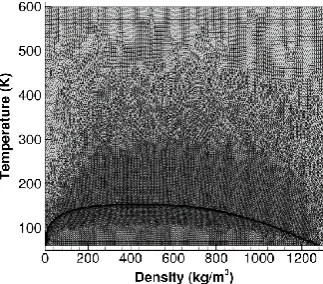
[31]). From equation (2) all the thermodynamic properties can be obtained, such as pressure, internal energy, enthalpy and speed of sound as a function of density and temperature. The saturation conditions are identified by the Maxwell criterion and the fluid properties in the saturation dome are calculated by the mixture assumption, whereas the mixture speed of sound is determined from the Wallis speed of sound formula [32]. In Fig. 1 phase diagrams for Oxygen are indicatively shown.
Instead of solving the Helmholtz EoS at each time step, a tabulated data technique, similar to Dumbser et al. [6] has been implemented after explicitly solving the RANS equations. An unstructured thermodynamic grid of approximately 34,000 thermodynamic elements has been created, which contains information for all the thermodynamic properties on each node. The thermodynamic grid is refined around the saturation curve, as it can be seen in Fig. 2.
(pressure, temperature or speed of sound) within a specific element of the table is then approximated by a Finite Element bilinear interpolation:
nodes
n,e Nn ,e bn
(3)Where b are the unknown coefficients of φ and N is the shape function of node n:
n n n n n
N ρ,e = 1+(e - e )+(ρ - ρ )+(e - e )(ρ - ρ ) (4) And the coefficients of each property are calculated by:
1N
b = (5)
Where φ are the values of the property at the nodes of the quadrilateral element and the shape function N of node n evaluated at node m is given by:
mn m n m n m n m n
N = 1+(e - e )+(ρ - ρ )+(e - e )(ρ - ρ ) (6)
[image:5.595.87.507.350.486.2]A Mach number consistent numerical flux has been implemented [5], [7] in order to handle the great variation of the Mach number between the different flow regimes, from incompressible flow in the liquid region, to highly compressible in the vapour and mixture regimes. A four-stage Runge-Kutta method, 4th order in time [33] has been selected for time discretisation.
Figure 1: Three dimensional phase diagrams for Oxygen: pressure (left), speed of sound (middle) and internal energy (right) in terms of density and temperature, combined with the saturation curve (dashed line). Properties
have been derived from Helmholtz EoS.
[image:5.595.216.378.546.688.2]3 RESULTS
In this section, the numerical model is firstly validated against the Riemann problem and a converging-diverging nozzle at cryogenic flow conditions and then, a RANS simulation of a conical converging-diverging nozzle is performed. The Riemann problem was selected as a means of validation of the spatial and temporal accuracy of the algorithm and to examine if it is feasible to capture the correct wave pattern. Next, the Euler equations have been also solved for a symmetrical converging-diverging nozzle, before advancing to more complicated RANS simulations of a conical nozzle, for which experimental data exist [12].
3.1 Riemann problem
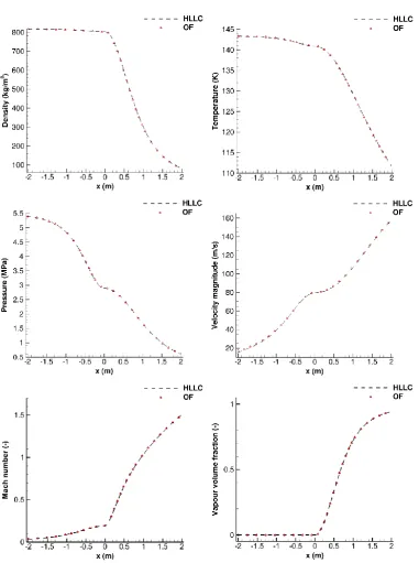
The first case examined is the Riemann problem in the computational domain x[-2,2 m] with initial conditions for the left state: ρL=965.8 kg/m3, TL=208.9 K, uL=0 m/s and for the right state: ρR=417.6 kg/m3, TR=111 K, uR=0 m/s. The numerical solution is compared with the solution from an 1-D FV solver which has been validated against the exact solution at time t=1 ms (Fig. 3). First order of spatial accuracy with 1000 equally spaced cells in the x direction has been used in both solvers. Wave transmissive boundary conditions have been employed for the
left and the right side of the shock tube, that is Un1
xL
Un
xL
and
1 0 0 n n x x U U .
As it can be seen in Fig. 3, the two solutions are in satisfactory agreement and the correct wave pattern has been successfully captured: a left moving expansion wave on the left, a contact discontinuity in the middle and a right moving shock wave on the right. It has to be mentioned here that although the same amount of computational cells and the same spatial accuracy is used in both solvers, dispersion is obvious in the traditional HLLC solver at the location of the right moving wave at x0.2m. This is a good demonstration of the capabilities of the Mach consistent numerical flux, which gives smooth and accurate solutions.
3.2 Converging-diverging nozzle
The second case examined is inviscid flow inside a symmetrical converging-diverging nozzle of circular cross-section S for x[-2,2 m] . The cross-section area varies with the length of the nozzle following the formula: for S x( )0.01x2 0.01. The inlet conditions are
3
817.07 /
in kg m
,T 143K, which will lead to an inlet pressure pin 5387100Pa, whereas in the outlet condition, only the pressure is specified, pout 1634699.75Pa. An inviscid simulation of a wedge of 5 degrees has been employed instead of simulating the whole nozzle. A structured grid of approximately 5200 cells has been created, where the length size is around
1
x cm
, equally spaced in the x-direction and y 4.3mm, equally spaced in the y-direction (Δy changes in the x direction, as the radius of the nozzle decreases or increases).
a pseudo 1-D FV solver coincide for all the plotted quantities. Due to subsonic flow conditions in the entrance, flow accelerates in the converging part. In the diverging part, flow continues to accelerate (M>1), resulting in further depressurization and beginning of vaporization. The supersonic region in this configuration is extended all the way down until the exit and no shock wave is noticed.
Figure 4: Validation for the converging-diverging nozzle case: comparison of the density (upper left), temperature (upper right), pressure (middle left), velocity magnitude (middle right), Mach number (lower left)
3.3 Conical converging-diverging nozzle
In order to demonstrate the applicability of the tabulated data algorithm in turbulent flows, a RANS simulation for a conical converging-diverging nozzle is performed (Reinflow=65k) and
[image:9.595.75.526.240.390.2]the obtained results are compared with experimental data of Hendricks et al. [12]. A wedge of 5 degrees is simulated, taking advantage of the problem symmetry; the nozzle geometry is demonstrated in Fig. 5. In the inflow, the total pressure is specified ptot,in=1.1385 MPa, whereas in the outlet the static pressure is pout=0.26 MPa. The k-ω SST turbulence model with the Reboud correction has been employed and the turbulence variables have been initialized accordingly, based on the Reynolds number in the inflow.
Figure 5: Geometry of the conical converging-diverging nozzle [12]. The inflow has been expanded upstream in order to impose the stagnation conditions of the experiment. The grey area denotes the computational domain,
whereas inlet and outlet are coloured by blue and red respectively.
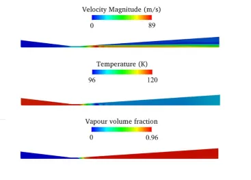
In Fig. 6 contour fields for the velocity magnitude, temperature and vapour volume fraction are shown. Similar to the previous case, the flow accelerates in the converging part before the throat, due to the subsonic flow conditions. Then a region of supersonic acceleration downstream the throat follows, which is terminated by a normal shock wave. The shock wave produces an instantaneous deceleration of the flow to subsonic speed. The subsonic flow decelerates through the remainder of the diverging section and exhausts as a subsonic jet. The vapour phase generated just after the throat region results in an increased Mach number (M=1.2). The mixture speed of sound here is determined by the Wallis formula [32] under the instantaneous phase change assumption. Almost full liquid vaporization has occurred after the throat, around x=0.015. The discrepancy of this point between the experiment and the simulation is responsible for predicting slightly different location of the shock wave (see also Fig. 7).
waves are noticed instead. Furthermore, in the inviscid simulation a pressure step is noticed at the location of the throat, which is not evident in the RANS simulation, due to numerical diffusion which is included from the turbulence modelling.
Figure 6: Contour fields for converging-diverging nozzle [10] RANS simulation: velocity magnitude (upper), temperature (middle) and vapour volume fraction (bottom).
Figure 7: Pressure distribution along x-axis for the conical converging-diverging nozzle; comparison between inviscid (dashed black), RANS (green) simulations and the experimental values (red square) of Hendricks et al.
[image:10.595.191.399.469.653.2]4 CONCLUSIONS
An explicit density based solver for cryogenic two-phase flows has been developed in OF. The Helmholtz EoS for oxygen has been employed in a tabulated form; finite element bilinear interpolation was used for approximating the thermodynamic properties. A Mach consistent numerical flux has been implemented allowing for large variation of its value along the computational domain. The numerical scheme has been validated against the Riemann problem and a pseudo 1-D finite volume solver for a symmetric converging-diverging nozzle. Then, RANS simulation of a conical converging-diverging nozzle has been performed and compared with experimental values. The results are satisfactory and the correct wave dynamics have been predicted in all the studied cases. This work demonstrates the applicability of the Helmholtz EoS in cryogenic flow conditions and RANS simulations.
REFERENCES
[1] T. Ramcke, A. Lampmann, and M. Pfitzner, “Simulations of Injection of Liquid Oxygen/Gaseous Methane Under Flashing Conditions,” Journal of Propulsion and
Power, pp. 1–13, Dec. 2017.
[2] Y. Liao and D. Lucas, “3D CFD simulation of flashing flows in a converging-diverging nozzle,” Nuclear Engineering and Design, vol. 292, pp. 149–163, Oct. 2015.
[3] J. Lee, R. Madabhushi, C. Fotache, S. Gopalakrishnan, and D. Schmidt, “Flashing flow of superheated jet fuel,” Proceedings of the Combustion Institute, vol. 32, no. 2, pp. 3215–3222, Jan. 2009.
[4] C. Greenshields, “OpenFOAM - The Open Source CFD Toolbox - User Guide,” May 2015.
[5] S. Schmidt, I. Sezal, G. Schnerr, and M. Talhamer, “Riemann Techniques for the
Simulation of Compressible Liquid Flows with Phase-Transistion at all Mach Numbers - Shock and Wave Dynamics in Cavitating 3-D Micro and Macro Systems,” in 46th AIAA
Aerospace Sciences Meeting and Exhibit, 0 vols., American Institute of Aeronautics and
Astronautics, 2008.
[6] M. Dumbser, U. Iben, and C.-D. Munz, “Efficient implementation of high order unstructured WENO schemes for cavitating flows,” Computers & Fluids, vol. 86, pp. 141–168, 5 2013.
[7] N. Kyriazis, P. Koukouvinis, and M. Gavaises, “Numerical investigation of bubble dynamics using tabulated data,” International Journal of Multiphase Flow, vol. 93, no. Supplement C, pp. 158–177, Jul. 2017.
[8] B. Chehroudi, D. Talley, and E. Coy, “Visual characteristics and initial growth rates of round cryogenic jets at subcritical and supercritical pressures,” Physics of Fluids, vol. 14, no. 2, pp. 850–861, 2002.
[9] G. Lamanna et al., “Flashing Behavior of Rocket Engine Propellants,” vol. 25, pp. 837–
856–837–856, Aug. 2015.
[10] R. C. Hendricks, R. J. Simoneau, and R. F. Barrows, “TWO-PHASE CHOKED FLOW OF SUBCOOLED OXYGEN AND NITROGEN,” Feb. 1976.
[12] L. Vingert, G. Ordonneau, N. Fdida, and P. Grenard, “A Rocket Engine under a Magnifying Glass,” Jan. 2016.
[13] H. Kim, H. Kim, D. Min, and C. Kim, “Numerical simulations of cryogenic cavitating flows,” Journal of Physics: Conference Series, vol. 656, no. 1, pp. 012131–012131, 2015.
[14] J. R. Travis, D. P. Koch, and W. Breitung, “A homogeneous non-equilibrium two-phase critical flow model,” International Journal of Hydrogen Energy, vol. 37, no. 22, pp. 17373–17379, 2012.
[15] G. B. Wallis, “Critical two-phase flow,” International Journal of Multiphase Flow, vol. 6, no. 1, pp. 97–112, 1980.
[16] S. Maksic and D. Mewes, “CFD-Calculation of the Flashing Flow in Pipes and Nozzles,” no. 36150, pp. 511–516, 2002.
[17] C. A. Marsh and A. P. O’Mahony, “Three-dimensional modelling of industrial flashing flows,” Progress in Computational Fluid Dynamics, an International Journal, vol. 9, no. 6–7, pp. 393–398, 2009.
[18] S. Mimouni, M. Boucker, J. Laviéville, A. Guelfi, and D. Bestion, “Modelling and computation of cavitation and boiling bubbly flows with the NEPTUNE_CFD code,” vol. 238, pp. 680–692, Mar. 2008.
[19] J. P. Janet, Y. Liao, and D. Lucas, “Heterogeneous nucleation in CFD simulation of flashing flows in converging–diverging nozzles,” International Journal of Multiphase Flow, vol. 74, pp. 106–117, 2015.
[20] Z. Bilicki and J. Kestin, “Physical aspects of the relaxation model in two-phase flow,”
Proceedings of the Royal Society of London A: Mathematical, Physical and Engineering
Sciences, vol. 428, no. 1875, pp. 379–397, 1990.
[21] D. P. Schmidt, S. Gopalakrishnan, and H. Jasak, “Multi-dimensional simulation of thermal non-equilibrium channel flow,” International Journal of Multiphase Flow, vol. 36, no. 4, pp. 284–292, 2010.
[22] I. K. Karathanassis, P. Koukouvinis, and M. Gavaises, “Comparative evaluation of phase-change mechanisms for the prediction of flashing flows,” International Journal of
Multiphase Flow, vol. 95, pp. 257–270, 2017.
[23] D. Fuster, G. Agbaglah, C. Josserand, S. Popinet, and S. Zaleski, “Numerical simulation of droplets, bubbles and waves: state of the art,” Fluid Dynamics Research, vol. 41, no. 6, pp. 065001–065001, 2009.
[24] Zwart, P. J., Gerber, A. G., and Belamri, T., “A Two-Phase Flow Model for Predicting Cavitation Dynamics.,” in ICMF 2004 International Conference on Multiphase Flow, 2004.
[25] A. H. Koop, “Numerical Simulation of Unsteady Three-Dimensional Sheet Cavitation,” University of Twente, 2008.
[26] G. Lamanna, H. Kamoun, B. Weigand, and J. Steelant, “Towards a unified treatment of fully flashing sprays,” International Journal of Multiphase Flow, vol. 58, pp. 168–184, 2014.
[27] R. B. Stewart, R. T. Jacobsen, and W. Wagner, “Thermodynamic Properties of Oxygen from the Triple Point to 300 K with Pressures to 80 MPa,” Journal of Physical and
[28] F. R. Menter, “Two-equation eddy-viscosity turbulence models for engineering applications,” AIAA Journal, vol. 32, no. 8, pp. 1598–1605, Aug. 1994.
[29] O. Coutier-Delgosha, R. Fortes-Patella, and J. L. Reboud, “Evaluation of the Turbulence Model Influence on the Numerical Simulations of Unsteady Cavitation,” Journal of
Fluids Engineering, vol. 125, no. 1, pp. 38–45, Jan. 2003.
[30] E. Lemmon, M. McLinden, and D. Friend, “NIST Chemistry WebBook, NIST Standard Reference Database Number 69,” 2005.
[31] R. Schmidt and W. Wagner, “A new form of the equation of state for pure substances and its application to oxygen,” Fluid Phase Equilibria, vol. 19, no. 3, pp. 175–200, Dec. 1985.
[32] Brennen C. E., Cavitation and Bubble Dynamics. 1995.
[33] E. F. Toro, Riemann Solvers and Numerical Methods for Fluid Dynamics, A Practical

![Figure 5: Geometry of the conical converging-diverging nozzle [12]. The inflow has been expanded upstream in order to impose the stagnation conditions of the experiment](https://thumb-us.123doks.com/thumbv2/123dok_us/1379860.91202/9.595.75.526.240.390/geometry-converging-diverging-expanded-upstream-stagnation-conditions-experiment.webp)