Efficient Implementation of Iterative Polynomial
Matrix EVD Algorithms Exploiting Structural
Redundancy and Parallelisation
Fraser K. Coutts,
Student Member, IEEE
, Ian K. Proudler, Stephan Weiss,
Senior Member, IEEE
Abstract—A number of algorithms are capable of itera-tively calculating a polynomial matrix eigenvalue decomposition (PEVD), which is a generalisation of the EVD and will diagonalise a parahermitian polynomial matrix via paraunitary operations. While offering promising results in various broadband array processing applications, the PEVD has seen limited deployment in hardware due to the high computational complexity of these algorithms. Akin to low complexity divide-and-conquer (DaC) solutions to eigenproblems, this paper addresses a partially par-allelisable DaC approach to the PEVD. A novel algorithm titled parallel-sequential matrix diagonalisation exhibits significantly reduced algorithmic complexity and run-time when compared with existing iterative PEVD methods. The DaC approach, which is shown to be suitable for multi-core implementation, can im-prove eigenvalue resolution at the expense of decomposition mean squared error, and offers a trade-off between the approximation order and accuracy of the resulting paraunitary matrices.
Index Terms—parahermitian matrix, paraunitary matrix, polynomial matrix eigenvalue decomposition, parallel, algorithm.
I. INTRODUCTION
T
HE eigenvalue decomposition (EVD) is a useful tool for many narrowband problems involving Hermitian in-stantaneous covariance matrices [1], [2]. In broadband ar-ray processing or multichannel time series applications, an instantaneous covariance matrix is not sufficient to measure correlation of signals across time delays. Instead, a space-time covariance matrix captures the auto- and cross-correlation sequences obtained from multiple time series. Itsz-transform, the cross-spectral density (CSD) matrix, is a Laurent polyno-mial matrix inz∈C[3], [4].A polynomial matrix eigenvalue decomposition (PEVD) has been defined as an extension of the EVD to parahermitian polynomial matrices in [5]. The PEVD uses finite impulse response (FIR) paraunitary matrices [6] to approximately diagonalise and typically spectrally majorise [7] a CSD matrix and its associated space-time covariance matrix. Recent work in [8], [9] provides conditions for the existence and uniqueness
This work was supported in parts by the Engineering and Physical Sciences Research Council (EPSRC) Grant number EP/S000631/1 and the MOD Uni-versity Defence Research Collaboration in Signal Processing. Fraser Coutts was the recipient of a Caledonian Scholarship by the Carnegie Trust.
F.K. Coutts is with the Institute for Digital Communications, School of Engineering, University of Edinburgh, Edinburgh, Scotland (e-mail [email protected]).
I.K. Proudler and S. Weiss are with the Centre for Signal & Im-age Processing (CeSIP), Department of Electronic & Electrical Engi-neering, University of Strathclyde, Glasgow G1 1XW, Scotland (e-mail
{ian.proudler,stephan.weiss}@strath.ac.uk).
of eigenvalues and eigenvectors of a PEVD, such that these can be represented by a power or Laurent series that is absolutely convergent, permitting a direct realisation in the time domain. Further research in [10] studies the impact of estimation errors in the sample space-time covariance matrix on its PEVD.
Once broadband multichannel problems have been ex-pressed using polynomial matrix formulations, solutions can be obtained via the PEVD. For example, the PEVD has been successfully used in broadband MIMO precoding and equalisation using linear [11]–[16] and non-linear [17], [18] approaches, broadband angle of arrival estimation [19]–[22], broadband beamforming [23]–[25], optimal subband cod-ing [7], [26], joint source-channel codcod-ing [27], source sep-aration [28], and scene discovery [29].
Existing PEVD algorithms include second-order sequential best rotation (SBR2) [5], sequential matrix diagonalisation (SMD) [30], and various evolutions of both algorithm fam-ilies [31]–[33]. Different from fixed order time domain PEVD schemes in [34], [35] and DFT-based approaches in [36]–[38], the SBR2 and SMD algorithm families have proven conver-gence. Both SBR2 and SMD algorithms employ iterative time domain schemes to approximately diagonalise a parahermitian matrix, and encourage — or even guarantee [39] — spectral majorisation such that the power spectral densities (PSDs) of the resulting eigenvalues are ordered at all frequencies [7].
While offering promising results, the PEVD has seen limited deployment in hardware. A parallel form of SBR2 whose performance has little dependency on the size of the input parahermitian matrix has been designed and implemented on an FPGA [40]–[42], but the SMD algorithm, which can achieve superior levels of diagonalisation [30], has been restricted to software applications due to its high computa-tional complexity and non-parallelisable architecture. Efforts to reduce the algorithmic cost of iterative PEVD algorithms, including SMD, have mostly been focussed on the trimming of polynomial matrices to curb growth in order [5], [43]– [45], which translates directly into a growth of computational complexity. By applying a row-shift truncation scheme for paraunitary matrices in [45]–[47], the polynomial order can be reduced with little loss to paraunitarity of the eigenvectors. These efforts, including a low cost cyclic-by-row numerical approximation of the EVD [48], [49] and optimisation over reduced parameter sets [33], [49], [50] have nonetheless not been able to reduce computational cost sufficiently to invite a hardware realisation.
cost of SMD-type algorithms through a novel combination and extension of recent numerical optimisation approaches. The structural redundancy inside the parahermitian matrix, i.e. its inherent symmetry, can be exploited in order to reduce both computations and memory requirements [51]. A divide-and-conquer (DaC) PEVD algorithm in [52] segments a large parahermitian matrix into multiple independent parahermitian matrices, which are subsequently diagonalised independently and simultaneously, demonstrating promising performance characteristics in applications [22], [47]. In the approach presented in this paper, both the ‘divide’ and ‘conquer’ stages make use of algorithmic improvements from [51] and [53], and the truncation schemes from [44], to minimise algorithm complexity. The final stage of the algorithm employs a novel variant of the row-shift truncation scheme of [45] to reduce the polynomial order of the paraunitary matrix.
Below, Sec. II will provide a summary of the notations and definitions used throughout this paper. Sec. III will introduce polynomial matrix truncation schemes used within the pro-posed parallel-sequential matrix diagonalisation (PSMD) ap-proach. The PSMD algorithm approach is outlined in Sec. IV, and performance metrics are defined in Sec. V. Simulation results for PSMD are compared to existing iterative PEVD methods in Sec. VI, with comments on hardware implemen-tations in Sec. VII and conclusions drawn in Sec. VIII.
II. NOTATIONS ANDDEFINITIONS
In this paper, upper- and lowercase boldface variables, such as A and a, refer to matrix- and vector-valued quantities, respectively. A dependency on a continuous and discrete variable is indicated via brackets and parentheses, respectively, such as A(t), t ∈ R, or a[n], n∈ Z. Polynomial quantities are denoted by their dependency on z and italic font, such as A(z). The expectation operator is denoted asE{·} and{·}H
indicates a Hermitian transpose. The parahermitian conjugate
{·}Pimplies a Hermitian transpose and a time reversal, such
that RP(z) =RH(1/z∗)[4].
In a broadband array scenario, a space-time covariance matrix
R[τ] =E{x[n]xH[n−τ]}
can be constructed from a vector-valued time-series x[n] ∈
CM, which depends on the discrete time index n and is assumed to be zero mean. Auto-correlation functions of theM
measurements inx[n]reside along the main diagonal ofR[τ], while cross-correlation terms between the different entries of
x[n]form the off-diagonal terms, such that R[τ] =RH[−τ].
The CSD matrixR(z) :C→CM×M arises as thez-transform of a space-time covariance matrix R[τ], NO FORMULA R(z) = PT
τ=−TR[τ]z
−τ, where T is the maximum lag of
R[τ]; i.e., R[τ] = 0 ∀ |τ| > T. The relationship between time domain and transform domain quantities is abbreviated below as R(z)•—◦R[τ]. Since R[τ] = RH[−τ], R(z) is
a parahermitian matrix, such that R(z) = RP(z) [4]. The PEVD [5] uses a paraunitary matrix F(z) to approximately diagonalise a parahermitian CSD matrixR(z)such that
R(z)≈FP(z)D(z)F(z), (1)
whereD(z)≈diag{D1(z), D2(z), . . . , DM(z)} approxi-mates a diagonal matrix and is typically spectrally majorised with PSDs Di(ejΩ) ≥ Di+1(ejΩ) ∀ Ω, i = 1. . .(M −1),
where Di(ejΩ) =Di(z)|z=ejΩ. The diagonal of D(z) con-tains approximate polynomial eigenvalues, and the rows of F(z)are approximate polynomial eigenvectors. The parauni-tary property of the eigenvectors ensures that
F(z)FP(z) =FP(z)F(z) =IM , (2) where IM is an M × M identity matrix. Note that the decomposition in (1) is unique up to permutations and arbitrary all-pass filters applied to the eigenvectors.
Equation (1) has only approximate equality, as the PEVD of a finite order polynomial matrix is generally transcendental, i.e. not of finite order; however, the approximation error can be shown to become arbitrarily small if the order of the approximation is selected sufficiently large [8]. A finite order approximation will therefore lead to only approximate diago-nality ofD(z) in (1). Similarly, a finite order approximation of F(z) through trimming will result in only approximate equality in (2).
By partitioning a parahermitian matrixR(z), it is possible to write
R(z) =R(−)(z) +R[0] +R(+)(z),
where R[0] is the ‘lag zero’ matrix of R(z), R(+)(z) con-tains terms for positive lag elements only, and R(−)(z) = R(+),P(z) [51]. It is therefore sufficient to record half of R(z), which here without loss of generality isR[0]+R(+)(z). For the remainder of this paper, we use the notation {·} to represent the recorded half of a parahermitian matrix; i.e., R(z) =R[0] +R(+)(z)andR(z)•—◦R[τ], where
R[τ] =
R[τ], 0≤τ≤T ;
0, otherwise.
If we possess knowledge of R(z), we have all the infor-mation required to obtain R(z), R[τ], and R[τ]. Given this relationship, we therefore refer to R(z) as a parahermitian matrix throughout this paper for brevity. In addition, we refer to R(z) and R[τ] as the ‘half-matrix’ versions of the ‘full-matrix’ representationsR(z)andR[τ], respectively.
Throughout this paper, Rm,k[τ]◦—•Rm,k(z) repre-sents the element in the mth row and kth column of
R[τ]◦—•R(z).
III. POLYNOMIALMATRIXTRUNCATIONSCHEMES
A. State-of-the-Art in Polynomial Matrix Truncation
The polynomial matrix truncation method from [44] is employed within PSMD. This approach reduces the order of a polynomial matrixY(z)— which has minimum lagT1and
maximum lagT2— by removing theT3(µ)leading andT4(µ)
trailing lags using a trim function
ftrim(Y[τ], µ) =
Y[τ], T1+T3(µ)≤τ ≤T2−T4(µ)
0, otherwise.
The amount of energy lost by removing the T3(µ) leading
and T4(µ) trailing lags of Y[τ] via theftrim(·) operation is
measured by
γtrim= 1−
P
τkftrim(Y[τ], µ)k2F
P
τkY[τ]k
2 F
, (4)
where k · kF is the Frobenius norm. A parameter µ is used
to provide an upper bound for γtrim. Given the above, the
truncation procedure can be expressed as the constrained optimisation problem:
maximise(T3(µ) +T4(µ)), s.t. γtrim≤µ . (5)
This is implemented by removing the outermost matrix co-efficients of matrix Y(z) until γtrim approaches µ from
below. Note that if Y(z) is parahermitian, T1 = −T2 and
T3(µ) =T4(µ)due to symmetry.
B. Compensated Row-Shift Truncation Method
The row-shift truncation method [45], [46] exploits ambi-guity in the paraunitary matrices [45], [54]. This arises as a generalisation of a phase ambiguity inherent to eigenvectors from a standard EVD [2], which in the polynomial case extends to arbitrary phase responses or all-pass filters. The simplest manifestation of such filters is of the form of an integer number of unit delays. If D(z) is exactly diagonal, then this phase ambiguity may permit eigenvectors F(z) to be replaced by a lower order Fˆ(z), whereFˆ(z) =Γ(z)F(z) andΓ(z)is a paraunitary diagonal matrix. In this case, since diagonal matrices commute,
R(z)≈FP(z)D(z)F(z) = ˆFP(z)Γ(z)D(z)ΓP(z)Fˆ(z) = ˆFP(z)D(z)Fˆ(z), (6) and D(z) in unaffected. The row-shift truncation method in [45] exploits this by searching for the best delay and truncation of all eigenvector approximations in a paraunitary matrix F(z)calculated by any PEVD algorithm.
During the iterations of a PEVD algorithm, or due to large M, the diagonalisation of D(z) may be poor with significant non-zero off-diagonal elements, such thatΓ(z)does not cancel as in (6). Since we are typically only interested in the approximate polynomial eigenvalues stored on the diagonal ofD(z), we propose a compensated variation of the row-shift truncation in [45] which incorporates the matrixΓ(z)into the parahermitian matrix to avoid propagating the decomposition error that would otherwise arise from neglecting non-zero off-diagonal components. Define the augmented parahermitian matrix Dˆ(z) = Γ(z)D(z)ΓP(z), so that the decomposition accuracy can now be maintained while using the lower order
ˆ
F(z) , s.t. R(z) ≈ FˆP(z)Dˆ(z)Fˆ(z). Note that because of
paraunitarity of Γ(z), Dˆ(z) possesses the same polynomial eigenvalues as D(z). While Dˆ(z) may now have a higher polynomial order than D(z), a suitable choice for Γ(z) can lead to an order reduction of the paraunitary matrix, which is typically more important for application purposes [17], [22], [24], [26], [27].
From [45], Γ(z)can take the form
Γ(z) = diag{zτ1, zτ2, . . . , zτM}. (7)
The delay matrixΓ(z)has the effect of shifting themth row of the paraunitary matrix F(z) by τm. These row shifts can be used to align the first polynomial coefficients in each row of the paraunitary matrix following the independent truncation of each row via the process below.
The matrixF(z)can be subdivided into itsM row vectors fm(z) :C→C1×M,m= 1. . . M,
F(z) =
f1(z) .. . fM(z)
.
Each row — which has minimum lag T1,m and maximum lag T2,m — is then truncated individually according to
ftrim(fm[τ], µ). The row shifts,τm, in (7) are then set equal to (T1,m+T3,m(µ)), m = 1. . . M, such that the minimum lag of each shifted row fˆm(z) is zero. Here, T3,m(µ) is the T3(µ)obtained via (3) for the mth row. Following
row-shift truncation, each row ofFˆ(z) has orderTm(µ), and the order of the paraunitary matrix is max
m=1...M{Tm(µ)}, where
Tm(µ) = T2,m −(T3,m(µ) + T4,m(µ)), with T3,m(µ) and
T4,m(µ)obtained from (5).
When applying compensated row-shift truncation (CRST) to a matrixF(z), we therefore obtain
[Fˆ(z),Dˆ(z)]←fCRST(F(z),D(z), µ),
withFˆ(z)having rowsfˆm(z)•—◦ˆfm[τ] =ftrim(fm[τ], µ). IV. PARALLEL-SEQUENTIALMATRIXDIAGONALISATION
Motivated by the results obtained by a DaC algorithm in [22], [47], this section outlines the components of a novel parallel-sequential matrix diagonalisation (PSMD) PEVD al-gorithm, which is summarised in Sec. IV-A. Sec. IV-B and Sec. IV-C explain its ‘divide’ and ‘conquer’ steps, respectively. Some comments on algorithm convergence are provided in Sec. IV-D.
A. Overview
The PSMD algorithm diagonalises a parahermitian matrix R(z) : C → CM×M via a number of paraunitary op-erations. The algorithm outputs an approximately diagonal matrix D(z), which contains the approximate eigenvalues, and an approximately paraunitary matrixF(z), which contains the corresponding approximate eigenvectors, such that (1) is satisfied.
diagonalised independently and simultaneously. Fig. 1 shows the state of the parahermitian matrix at each stage of the process for this example. As in [51], here we exploit the natural symmetry of the parahermitian matrix structure and only store one half of its elements; i.e., we diagonaliseR(z).
Research in [49], [55] has shown that restricting the search space of iterative PEVD algorithms to a subset of lags around lag zero of a parahermitian matrix can bring performance gains with little impact on algorithm convergence. To reduce the computational complexity, we therefore employ the restricted update method of [53] in the ‘divide’ and ‘conquer’ stages. This not only restricts the search space of the algorithms used in each stage, but also restricts the portion of the parahermitian matrix that is updated at each iteration.
If R(z) is of large spatial dimension, an algorithm named half-matrix restricted update sequential matrix segmentation (HRSMS) is repeatedly used to ‘divide’ the matrix into block diagonal form that contains multiple independent parahermi-tian matrices. This function generates a paraunitary matrix T(z)that ‘divides’ an input matrixA(z)into two independent parahermitian matrices,A11(z)andA22(z), of smaller spatial
dimension.A11(z)is then subject to further ‘division’ if it still
has sufficiently large spatial dimension. Following a number of ‘division’ steps, each of the output independent parahermitian matrices are stored on the diagonal of matrix R0(z); thus, R0(z) is block diagonal by construction. The matrices T(z) are concatenated to form an overall dividing matrix G(z). It is therefore possible to approximately reconstruct R(z)from the product GP(z)R0(z)G(z).
Each block on the diagonal of matrix R0(z)is then diago-nalised in parallel through the use of a half-matrix version of the algorithm from [53], named half-matrix restricted update sequential matrix diagonalisation (HRSMD). The diagonalised outputs,C(z), are placed on the diagonal of matrixD(z), and the corresponding paraunitary matrices, V(z), are stored on the diagonal of matrixJ(z). The matrixR0(z)can be approxi-mately reconstructed fromJP(z)D(z)J(z); by extension, it is possible to approximately reconstructR(z)from the product GP(z)JP(z)D(z)J(z)G(z) =FP(z)D(z)F(z).
The polynomial matrix truncation scheme of Sec. III-A is implemented within HRSMS and HRSMD. The paraunitary matrix compensated row-shift truncation scheme of Sec. III-B is more costly than the method of Sec. III-A, and does not pro-vide an increase in truncation performance when implemented within the SMD algorithm [46] — which the aforementioned algorithms are based on. However, a similar strategy has been found to be effective when truncating the output paraunitary matrix of a DaC PEVD scheme in [47]. Similarly, we employ this scheme to truncate the final paraunitary matrix in PSMD. Algorithm 1 summarises the above steps of PSMD in more detail. Of the parameters input to PSMD, µ,µt, and µs are truncation parameters, andδandare stopping thresholds for HRSMS and HRSMD, which are allowed a maximum of ID and IC iterations. Matrices of spatial dimension greater than
ˆ
M ×Mˆ will be subject to ‘division’. The parameter P will be discussed in subsequent sections; IM and0M are identity and zero matrices of spatial dimensionsM×M, respectively.
a)
=
=TR
=
=TR
b) c)
=
[image:4.612.311.564.54.129.2]=TD
Fig. 1. Concept of PSMD: (a) original matrixR[τ]∈C20×20, which in a first ‘divide’ paraunitary similarity transform step yields (b) the block diagonal resultR0[τ]; a second paraunitary similarity transform, which can now be applied to each subblock separately leads to (c) the diagonalised outputD[τ].
Input:R(z),µ,µt,µs,δ,,ID,IC,Mˆ,P Output: D(z),F(z)
Determine if input matrix is large: ifM >Mˆ then
Large matrix — ‘divide-and-conquer’:
M0←M,A(z)←R(z),G(z)←IM, R0(z),J(z),D(z)←0M, α←0 ‘Divide’ matrix:
whileM0 >Mˆ do
α←α+ 1
[A11(z),A22(z),T(z)]←
HRSMS(A(z), ID, P, δ, µ, µt)
(M−M0) ones appended to lag zero diagonal ofT(z)to formTˆ(z)
StoreA22(z)on diagonal of R0(z)inαth
P×P block from bottom-right
G(z)←Tˆ(z)G(z),A(z)←A11(z),
M0←M0−P
end
StoreA(z)on diagonal ofR0(z)in top-left
M0×M0 block
‘Conquer’ independent matrices (in parallel):
forγ←1to (α+ 1)do
B(z)isγth block ofR0(z)from bottom-right [C(z),V(z)]←HRSMD(B(z), IC, , µ, µt) Store(C(z),V(z))inγth block of
(D(z),J(z))from bottom-right end
F(z)←J(z)G(z) else
Small matrix — perform HRSMD only: [F(z),D(z)]←HRSMD(R(z), IC, , µ, µt) end
D[τ]←ftrim(D[τ], µ)
Apply compensated row-shift truncation: [F(z),D(z)]←fshift(F(z),D(z), µs)
Algorithm 1: PSMD Algorithm
B. ‘Dividing’ the Parahermitian Matrix
a)
=
=
T
A=
b)
A]
A22]
A2]
A2
]
=
T
AFig. 2. (a) Original matrixA[τ]∈ C20×20 with regions to be driven to
zero in HRSMS, and (b) segmented result forP = 4;TAandTA0 are the maximum lags for the original and segmented matrices, respectively.
variant of SMD [30] designed to segment a matrix A(z) : C → CM
0×M0
into two independent parahermitian matrices A11(z) :C→C(M
0−P)×(M0−P)
and A22(z) :C→CP×P, and two matrices A12(z) : C → C(M
0−P)×P
and A21(z) :
C → CP×(M
0−P)
, where A12(z) = AP21(z) approximates
a matrix of zeroes. The dimensions of the smaller matrix produced during division, P, is forced to satisfy P ≤ Mˆ. Each instance of HRSMS is provided with a parameter ID — which defines the maximum possible number of algorithm iterations — a stopping thresholdδ, and truncation parameters
µ andµt.
To achieve matrix segmentation, the HRSMS algorithm uses a series of elementary paraunitary operations to iteratively minimise the energy in the bottom-left P ×(M0−P) and top-right (M0 −P)×P regions of A(z). Each elementary paraunitary operation consists of two steps: first a delay step is used to move the region with the largest energy to lag zero; then an EVD diagonalises the lag zero matrix, transferring the shifted energy onto the diagonal.
[image:5.612.60.285.54.153.2]We employ the restricted update method of [53] in HRSMS, which calculates the paraunitary matrix while restricting the search space of the algorithm and the portion of the para-hermitian matrix that is updated at each iteration. This re-striction limits both the number of search operations and the computations required to update the increasingly segmented parahermitian matrix. Over the course of algorithm iterations, the update space contracts piecewise strictly monotonically. That is, the update space contracts until order zero is reached; after this, in a so-called regeneration step, the calculated paraunitary matrix is applied to the input matrix to construct the full-sized parahermitian factor. The update space is then maximised and thereafter again contracts monotonically over the following iterations.
Fig. 2 illustrates the segmentation process of HRSMS for
M0 = 20 and P = 4. In this example, if M0−P = 16 is greater than Mˆ,A11[τ] will be subject to further division.
Upon initialisation, the algorithm diagonalises the lag zero coefficient matrix A[0] by means of its modal matrix Q(0),
which is obtained from the ordered EVD of A[0], such that S(0)(z) =Q(0)A(z)Q(0),H. The unitaryQ(0)is applied to all coefficient matrices A[τ]∀ τ ≥0, and initialisesH(0)(z) =
Q(0).
Although the HRSMS algorithm operates on S(i)(z), it
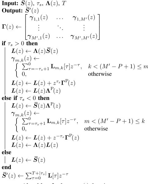
Input:S(z),τs,Λ(z),T Output: S0(z)
Γ(z)←
γ1,1(z) . . . γ1,M0(z) ..
. . .. ...
γM0,1(z) . . . γM0,M0(z)
ifτs>0 then
L(z)←Λ(z)S(z) γm,k(z)←
P0
τ=−τs+1Lm,k[τ]z
−τ, k <(M0−P+ 1)≤m
0, otherwise
L(z)←L(z) +zτsΓP(z) L(z)←L(z)ΛP(z) else ifτs<0 then
L(z)←S(z)ΛP(z)
γm,k(z)← P0
τ=τs+1Lm,k[τ]z
−τ, m <(M0−P+ 1)≤k
0, otherwise
L(z)←L(z) +z−τsΓP(z) L(z)←Λ(z)L(z)
else
L(z)←S(z) end
S0(z)←PT+|τs| τ=0 L[τ]z
−τ
Algorithm 2: fshift,SMS(·)function
effectively computes
S(i)(z) =U(i)(z)S(i−1)(z)U(i),P(z) H(i)(z) =U(i)(z)H(i−1)(z)
in theith step,i= 1,2, . . .min{ID, I}, in which
U(i)(z) =Q(i)Λ(i)(z), (8) and I is defined later. The product in (8) consists of a paraunitary delay matrix
Λ(i)(z) = diag{1 . . . 1
| {z }
M0−P
zτ(i) . . . zτ(i) | {z }
P
} (9)
and a unitary Q(i), with the result that U(i)(z)
in (8) is paraunitary. For subsequent discussion, it is convenient to define intermediate variablesS(i)0(z)andH(i)0(z)
where
S(i)0(z) =fshift,SMS(S(i−1)(z), τ(i),Λ(i)(z), T(i−1))
H(i)0(z) =Λ(i)(z)H(i−1)(z) , (10) wherefshift,SMS(·)— which is described in Algorithm 2 —
implements the delays encapsulated in the matrixΛ(i)(z)for a half-matrix representation andT(i−1)is the maximum lag of
S(i−1)[τ]. MatrixΛ(i)(z)is selected based on the position of
the dominant region inS(i−1)(z)•—◦S(i−1)[τ], as identified
by the parameter set
τ(i)= arg max τ
kS(21i−1)[τ]kF, kS (i−1)
[image:5.612.319.561.56.357.2]b)
d)
e) a)
= 3
= 2 = 1
= 0
c)
= 3
= 2 = 0
= 1
= 3
= 2 = 0
[image:6.612.48.565.52.276.2]= 1
Fig. 3. Example for a matrix where in theith iteration the Frobenius norm of a region in the top-right of the matrix is maximum: (a) the region is shifted (here in negative direction), with elements in the region past lag zero (b) extracted and (c) parahermitian conjugated; (d) these elements are appended to the far (hidden) bottom-left region at lag zero and (e) shifted in the opposite (here positive) direction.
where
kS(21i−1)[τ]kF=
v u u t
M0
X
m=M0−P+1 M0−P
X
k=1
|S(m,ki−1)[τ]|2,
and the norm of kS(12i−1)[τ]kF is similarly calculated over the
terms S(k,mi−1)[τ].
According to the fshift,SMS(·) function: if (11) returns
τ(i) > 0, then the bottom-left P ×(M0 −P) region of S(i−1)(z) is to be shifted by τ(i) lags towards lag zero. If
τ(i)<0, it is the top-right(M0−P)×P region that requires shifting by−τ(i) lags towards lag zero. To preserve the
half-matrix representation, elements that are shifted beyond lag zero, i.e., outside the recorded half-matrix, have to be stored as their parahermitian conjugate (i.e., Hermitian transposed and time reversed) and appended onto the bottom-leftP×(M0−P) (forτ(i)<0) or top-right(M0−P)×P(forτ(i)>0) region of
the shifted matrix at lag zero. The concatenated region is then shifted by |τ(i)| elements towards increasingτ. Note that the
fshift,SMS(·)function shifts the bottom-rightP×P region of
S(i−1)(z)in opposite directions, such that this region remains unaffected. An efficient implementation of fshift,SMS(·) can
therefore exclude this region from shifting operations. An efficient example of the shift operation is depicted in Fig. 3 for the case of S(i−1)(z) :
C→C5×5 with parameters
τ(i)=−3,T(i−1)= 3, andP = 2. Owing to the negative sign
of τ(i), it is here the top-right(M0−P)×P region that has to be shifted first, followed by the bottom-leftP×(M0−P) region, which is shifted in the opposite direction.
The shifting process in (10) moves the dominant bottom-left or top-right region inS(i−1)[τ]into the lag zero coefficient ma-trix S(i)0[0]. In accordance with the restricted update scheme of [53], we now obtain a matrix
S(i)00(z) =
T(i−1)−|τ(i)|
X
τ=0
¯
S(i)0[τ]z−τ. (12)
Note that S(i)00(z) is not equal to S(i)0(z) by construction but is of lower order and therefore less computationally costly to update in the subsequent step. Applying (12) at
a) = 3
= 2
= 1
=
= 3
= 2
= 1
=
= 2
= 1
=
b) c)
= 2
= 1
=
d)
= 2
= 1
=
= 1
=
e) f)
= 1
=
g)
= 1
=
h)
=
i)
Fig. 4. (a) MatrixS(i−1)(z) :
C→C5×5 with maximum lagT(i−1)= 3 andP = 2; (b) shifting of region with maximum energy to lag zero (τ(i)=
−1); (c) central matrix with maximum lag(T(i−1)− |τ(i)|) = 2,S(i)00(z), is extracted. (d)S(i)(z) =Q(i)S(i)00(z)Q(i),H; (e) shifting of region with maximum energy to lag zero (τ(i+1) = 1); (f)S(i+1)00(z)extracted. (g) S(i+1)(z); (h)τ(i+2)=−1; (i)S(i+2)00(z)is extracted.
each iteration enforces a monotonic contraction of the update space of the algorithm. We can therefore avoid truncation of S(i)00(z)at each iteration, as its order is not increasing. As a result of this, we also limit the search space of (11), which negatively impacts the convergence speed of HRSMS, as we may not identify the same τ(i) as an unrestricted version of
the algorithm. However, we demonstrate in Sec. VI that this impact is typically not significant.
The order of the paraunitary matrixH(i)0(z)does increase at each iteration; to constrain computational complexity, we obtain a truncated paraunitary matrix
H(i)00[τ] =ftrim(H(i)0[τ], µt).
The energy in the shifted regions is then transferred onto the diagonal of S(i)00[0] by a unitary matrix Q(i) — which
diagonalisesS(i)00[0]by means of an ordered EVD — in S(i)(z) =Q(i)S(i)00(z)Q(i),H
H(i)(z) =Q(i)H(i)00(z) . (13) If at this point the order of S(i)(z) is zero, we
obtain a regenerated parahermitian matrix S(i)(z) = H(i)(z)R(z)H(i),P(z), and truncate to minimise future computational complexity via S(i)[τ] ← f
trim(S(i)[τ], µ).
Note that obtaining the regenerated matrix requires the use of a full-matrix representation. Following regeneration, we can continue with a half-matrix representation.
Input:A(z),ID,P,δ,µ,µt Output: A11(z),A22(z),T(z)
Find eigenvectors Q(0) that diagonalise
A[0]∈CM
0×M0
S(0)(z)←Q(0)A(z)Q(0),H,H(0)(z)←Q(0),i←0, stop←0
do
i←i+ 1
Find τ(i) from (11); generateΛ(i)(z)from (9)
S(i)0(z)←
fshift,SMS(S(i−1)(z), τ(i),Λ(i)(z), T(i−1))
H(i)0(z)←Λ(i)(z)H(i−1)(z) S(i)00(z)←PT(i−1)−|τ(i)|
τ=0 ¯S(i)0[τ]z−τ
H(i)00[τ]←f
trim(H(i)0[τ], µt)
Find eigenvectors Q(i)that diagonaliseS(i)00[0] S(i)(z)←Q(i)S(i)00(z)Q(i),H
H(i)(z)←Q(i)H(i)00(z) if T(i)= 0 ori > I
D or(14) satisfiedthen S(i)(z)←H(i)(z)R(z)H(i),P(z)
S(i)[τ]←ftrim(S(i)[τ], µ)
end
if i > ID or (14) satisfiedthen stop ←1
end while stop= 0 T(z)←H(i)(z)
A11(z)is top-left(M0−P)×(M0−P)block ofS(i)(z)
A22(z) is bottom-rightP×P block ofS(i)(z)
Algorithm 3: HRSMS algorithm
After a user-defined ID iterations, or when
max τ
n
kS(21I)[τ]k2 F, kS
(I) 12[−τ]k
2 F
o
≤δX
τ
kR[τ]k2 F (14)
at some iterationI— whereδis chosen to be arbitrarily small — the HRSMS algorithm returns matrices A11(z), A22(z),
andT(z). The latter is constructed from the concatenation of the elementary paraunitary matrices:
T(z) =H( ˆI)(z) =U( ˆI)(z)· · ·U(0)(z) =
ˆ
I
Y
i=0
U( ˆI−i)(z),
where Iˆ= min{ID, I}.A11(z) is the top-left (M0 −P)×
(M0−P)block of A0(z) =T(z)R(z)TP(z)and A22(z)is
the bottom-right P×P block ofA0(z).
The above steps of HRSMS are summarised in Algorithm 3.
C. ‘Conquering’ the Independent Matrices
At this stage of PSMD, R(z) has been segmented into multiple independent parahermitian matrices, which are stored as blocks on the diagonal of R0(z). Each matrix can now be diagonalised individually through the use of a PEVD algo-rithm; here, a half-matrix version [51] of the restricted update SMD algorithm from [53] is chosen, and is henceforth named half-matrix restricted update sequential matrix diagonalisation
Input:B(z),IC,,µ,µt Output: C(z),V(z)
Find eigenvectorsQ(0) that diagonaliseB[0]∈
CN×N S(0)(z)←Q(0)B(z)Q(0),H,H(0)(z)←Q(0),i←0,
stop ←0 do
i←i+ 1
Find {c(i), τ(i)} from (16); generateΛ(i)(z)
from (15) S(i)0(z)←
fshift,SMD(S(i−1)(z), c(i), τ(i),Λ(i)(z), T(i−1))
H(i)0(z)←Λ(i)(z)H(i−1)(z) S(i)00(z)←PT(i−1)−|τ(i)|
τ=0 S¯(i)0[τ]z−τ
H(i)00[τ]←f
trim(H(i)0[τ], µt)
Find eigenvectorsQ(i) that diagonaliseS(i)00[0] S(i)(z)←Q(i)S(i)00(z)Q(i),H
H(i)(z)←Q(i)H(i)00(z) ifT(i)= 0ori > I
C or (18) satisfiedthen S(i)(z)←H(i)(z)R(z)H(i),P(z)
S(i)[τ]←ftrim(S(i)[τ], µ)
end
ifi > IC or (18) satisfiedthen stop←1;
end whilestop= 0 V(z)←H(i)(z) C(z)←S(i)(z)
Algorithm 4: HRSMD algorithm
(HRSMD). Each instance of HRSMD is provided with a parameterIC — which defines the maximum possible number of algorithm iterations — a stopping threshold , and trun-cation parameters µ and µt. Upon completion, the HRSMD algorithm returns matrices V(z) and C(z), which contain the polynomial eigenvectors and eigenvalues for input matrix B(z), respectively, such thatC(z) =V(z)B(z)VP(z).
The HRSMD algorithm approximates the PEVD using a series of elementary paraunitary operations to iteratively diagonalise a parahermitian matrixB(z) :C→CN×N. Each elementary paraunitary operation consists of two steps: first a delay step is used to move the column or row with the largest energy in its off-diagonal elements to lag zero; then an EVD diagonalises the lag zero matrix, transferring the shifted energy onto the diagonal.
The HRSMD algorithm is functionally very similar to HRSMS, and also employs the restricted update approach of [53]. HRSMS zeroes off-diagonal elements in order to create a block-diagonal matrix, whereas HRSMD zeroes off-diagonal elements in order to create a off-diagonal matrix. We therefore describe only the differences between HRSMD and HRSMS, and provide pseudocode in Algorithm 4.
In HRSMD, the product in (8) uses a paraunitary delay matrix
Λ(i)(z) = diag{1 . . . 1
| {z }
c(i)−1
z−τ(i) 1 . . . 1
| {z }
N−c(i)
Input:S(z),c,τs,Λ(z),T Output: S0(z)
Γ(z)←
γ1,1(z) . . . γ1,N(z) ..
. . .. ... γN,1(z) . . . γN,N(z)
if τs>0then
L(z)←S(z)ΛP(z) γm,k(z)←
P0
τ=−τs+1Lm,k[τ]z
−τ, k=c, m6=c
0, otherwise
L(z)←L(z) +zτsΓP(z) L(z)←Λ(z)L(z) else if τs<0 then
L(z)←Λ(z)S(z) γm,k(z)←
P0
τ=τs+1Lm,k[τ]z
−τ, m=c, k6=c
0, otherwise
L(z)←L(z) +z−τsΓP(z) L(z)←L(z)ΛP(z)
else
L(z)←S(z) end
S0(z)←PT+|τs| τ=0 L[τ]z
−τ
Algorithm 5: fshift,SMD(·)function
which is selected based on the position of the dominant off-diagonal column or row in S(i−1)(z)•—◦S(i−1)[τ], as
identified by the parameter set
{c(i), τ(i)}= arg max
k,τ
n
kˆs(ki−1)[τ]k2,kˆs (i−1) (r),k [−τ]k2
o ,(16)
where
kˆs(ki−1)[τ]k2=
q PN
m=1,m6=k|S
(i−1)
m,k [τ]|2,
kˆs((r)i−,k1)[τ]k2=
q PN
m=1,m6=k|S
(i−1)
k,m [τ]|2. (17) A function fshift,SMD(·) — described in Algorithm 5 — is
used instead of fshift,SMS(·). According to the fshift,SMD(·)
function: if (16) returns τ(i) > 0, then the c(i)th column of
S(i−1)(z) is to be shifted by τ(i) lags towards lag zero. If
τ(i) < 0, it is the c(i)th row that requires shifting by −τ(i)
lags towards lag zero. Elements that are shifted beyond lag zero have to be stored as their parahermitian conjugate and appended onto the c(i)th row (for τ(i) > 0) or column (for
τ(i)<0) of the shifted matrix at lag zero. The concatenated
row or column is then shifted by |τ(i)| elements towards
increasing τ. Note that the fshift,SMD(·) function shifts the
polynomial in thec(i)th position along the diagonal in opposite
directions, such that this polynomial remains unaffected. An efficient implementation offshift,SMD(·)can therefore exclude
this element from shifting operations.
Iterations of HRSMD continue for a maximum ofICsteps, or until S(I)(z)is sufficiently diagonalised — for someI —
with dominant off-diagonal column or row norm
max k,τ
n
kˆs(kI)[τ]k2, kˆs (I) (r),k[−τ]k2
o
≤ , (18)
where the value of is chosen to be arbitrarily small. On completion, HRSMD returns matricesV(z)andC(z), where C(z) =V(z)B(z)VP(z). The former is constructed from the concatenation of the elementary paraunitary matrices:
V(z) =H( ˆI)(z) =U( ˆI)(z)· · ·U(0)(z) =
ˆ
I
Y
i=0
U( ˆI−i)(z),
whereIˆ= min{IC, I}.
D. Algorithm Convergence
Various members of the SMD family of algorithms have been explicitly proven to converge in [30], [31], [56], and are guaranteed to reduce a norm over all off-diagonal elements of a parahermitian matrix below any arbitrarily small value, given a sufficient number of iterations. The algorithm family includes search space strategies that limit the temporal and/or spatial application of a paraunitary similarity transform [50], [56], which are similar to the spatial restrictions applied within the HRSMS ‘divide’ algorithm, and the HRSMD algorithm performing the ‘conquer’ step. Thus the PSMD algorithm only applies numerical efficiencies to these existing SMD family members, and provided that truncation errors are sufficiently low to not substantially alter the matrix factors, the PSMD algorithm’s convergence is covered by these existing proofs and formally summarised in [57], which is omitted here.
V. CONVERGENCEMETRICS
If HRSMS is not executed with a sufficient number of iterations ID or the threshold δ is too high, the generated parahermitian matrix is not perfectly block diagonal, with the matricesA21(z) andA12(z)containing non-zero energy.
Discarding the latter matrices upon completion of an instance of HRSMS introduces errors that degrade the approximation given by (1). Counteracting this by an increase in ID or de-crease ofδwill reduce the speed and increase the complexity of the ‘divide’ step and therefore the overall algorithm.
Further, higher truncation thresholds for the parahermitian and paraunitary matrices worsen the approximation given by (1) and weaken the paraunitary property of eigenvectors F(z); i.e., equality in (2) is no longer guaranteed if truncation is employed during generation ofF(z). We will define metrics for these errors below.
1) Normalised Off-Diagonal Energy : Since iterative PEVD algorithms progressively minimise off-diagonal energy, a suit-able metric Enorm(i) , defined in [30], can be used to measure
their performance; this metric normalises the off-diagonal energy in the parahermitian matrix at the ith iteration— equivalent to the square of (17)— by the total energy, which remains invariant under paraunitary operations. Computation of Enorm(i) generates squared covariance terms; therefore a
2) Eigenvalue Resolution: We define eigenvalue resolution as the normalised mean-squared error between the spectrally majorised ground-truth and measured eigenvalue PSDs:
λres=
1
M K
M
X
m=1
K−1
X
k=0
|Dm,m[k]−Wˆm,m[k]| ˆ
Wm,m[k]
, (19)
where D[k] is obtained from the K-point DFT of D[τ] and
ˆ
W[k] is found by spectrally majorising theK-point DFT of ground-truth eigenvaluesW[τ]. A suitableK is identified as the smallest power of two greater than the lengths of D(z) and W(z). The normalisation in (19) will give emphasis to the correct extraction of small eigenvalues in the presence of stronger ones, similar to the coding gain metric in [26].
3) Decomposition Mean Squared Error: Denote the mean squared reconstruction error for an approximate PEVD as
MSE = 1
M2L0
X
τkER[τ]k
2
F, (20)
where ER[τ] =Rˆ[τ]−R[τ], Rˆ(z) =FP(z)D(z)F(z), and
L0 is the length ofE R(z).
4) Paraunitarity Error: Define the paraunitarity error as
η= 1
M X
τkEF[τ]−IM[τ]k
2
F, (21)
where EF(z) = F(z)FP(z), IM[0] is an M ×M identity
matrix, andIM[τ]for τ6= 0 is anM ×M matrix of zeroes.
5) Paraunitary Filter Length: The output paraunitary ma-trix F(z) can be implemented as a lossless bank of finite impulse response filters in applications; a useful metric for gauging the implementation cost of this matrix therefore is its length, LF.
VI. SIMULATIONS ANDRESULTS
A. Simulation Scenario
The simulations below have been performed over an ensem-ble of 103 instantiations of R(z) : C → CM×M, M = 30, based on the randomised source model in [30]. This source model generates R(z) = XP(z)W(z)X(z), whereby the diagonal W(z) : C → CM×M contains the PSDs of 30 independent sources. These sources are spectrally shaped by innovation filters such that W(z) has an order of 118, and limits the dynamic range of the PSDs to about30 dB. Random paraunitary matricesX(z) :C→CM×M of order 60 perform a convolutive mixing of these sources, such that R(z)has an order of 238.
The performances of the existing SBR2 [5], SMD [30], and DCSMD [52] PEVD algorithms are compared with a newly developed half-matrix DCSMD (HDCSMD) algorithm and the proposed PSMD algorithm.
SBR2 and SMD are allowed to run for 1800 and 1400 iterations, respectively, with truncation parameters µSBR2 =
µSMD = 10−6. DCSMD, HDCSMD, and PSMD are provided
with parameters µ = µt = µs = 10−12, δ = 0, = 0,
ID = 100, IC = 200, Mˆ = 8, and P = 8. Two variants of PSMD are also tested: PSMD1 is supplied with
µ=µt=µs= 10−6and PSMD2 is supplied withID= 400, while all other parameters are kept the same.
0 2 4 6 8 10 12 14 16 18 20
−14 −12 −10 −8 −6 −4 −2 0
Time / s
5l
og
1
0
E
{
E
(
i
)
n
o
rm
}
/
[d
B
]
SBR2 SMD DCSMD HDCSMD PSMD PSMD1
PSMD2
1 1.5 2 −13.6
[image:9.612.315.562.61.151.2]−13.4
Fig. 5. Performance of PSMD, PSMD1, and PSMD2 relative to SBR2 [5], SMD [30], DCSMD [52], and half-matrix DCSMD for the decomposition of a30×30parahermitian matrix.
Simulations were performed within MATLABR R2014a under UbuntuR 16.04 on an MSIR GE60-2OE with IntelR CoreTMi7-4700MQ2.40 GHz×8cores, NVIDIAR GeForceR GTX 765M, and8 GB RAM.
B. Diagonalisation Speed
1) Without Parallelisation: The ensemble-averaged diago-nalisation metric of Sec. V-1 for each of the tested PEVD algorithms is plotted against the ensemble-averaged elapsed system time at each iteration in Fig. 5. The curves demonstrate that PSMD achieves a similar degree of diagonalisation to most of the other algorithms, but in a shorter time. The SBR2 algorithm exhibits relatively low diagonalisation with respect to time, and would require a great deal of additional simulation time to attain diagonalisation performance simi-lar to the other algorithms. By utilising a restricted update approach, PSMD has sacrificed a small amount of diago-nalisation performance to decrease algorithm run-time versus the otherwise functionally identical HDCSMD algorithm. In-creased levels of truncation within PSMD1 have decreased
algorithm run-time but have also decreased diagonalisation performance slightly. The increase in ID within PSMD2 has increased the run-time of the ‘divide’ step and marginally improved diagonalisation.
The ‘stepped’ characteristics of the curves for the DaC strategies of DCSMD, HDCSMD, and PSMD are a result of the algorithms’ two-stage implementation. The ‘divide’ steps of the algorithms exhibit low diagonalisation for a large increase in execution time. In the ‘conquer’ steps, high diagonalisation is seen for a small increase in execution time.
2) With Parallelisation: From Fig. 5, the average run-time for the PSMD algorithm for the given simulation scenario is 1.485 seconds. If the MATLABR Parallel Computing ToolboxTM is used to parallelise the ‘conquer’ step of PSMD by spreading four instances of HRSMD across the four cores present on the simulation platform, the average run-time can be reduced to 1.075 seconds. The performance of PSMD is otherwise identical.
TABLE I
AVERAGEλres, MSE,η,ANDLF COMPARISON.
Method λres MSE η LF
SBR2 [5] 1.1305 1.293×10⁻⁶ 2.448×10⁻⁸ 133.8
SMD [30] 0.0773 3.514×10⁻⁶ 6.579×10⁻⁸ 165.5 DCSMD [52] 0.0644 6.785×10⁻⁶ 1.226×10⁻¹⁴ 360.4 HDCSMD 0.0644 6.785×10⁻⁶ 1.226×10⁻¹⁴ 360.4
PSMD 0.0658 6.918×10⁻⁶ 4.401×10⁻¹⁵ 279.3 PSMD1 0.0661 8.346×10⁻⁶ 1.303×10⁻⁸ 156.0 PSMD2 0.0245 7.618×10⁻⁷ 1.307×10⁻¹⁴ 307.6
C. Eigenvalue Resolution
The ensemble-averaged eigenvalue resolution of (19) can be seen in column two of Tab. I. It can be observed that the DaC approaches to the PEVD offer superior eigenvalue resolution versus SMD, despite the fact that all algorithms bar SBR2 achieve similar levels of diagonalisation. The slightly worse diagonalisation performance of PSMD relative to DCSMD and HDCSMD has translated to marginally higher λres. The
poor diagonalisation performance of SBR2 has resulted in significantly worse resolution of the eigenvalues. Paired with its degraded diagonalisation performance, PSMD1has slightly
higherλresthan PSMD. While PSMD2achieves a similar level
of diagonalisation to PSMD, the additional effort contributed towards the ‘divide’ step has dramatically improved λres.
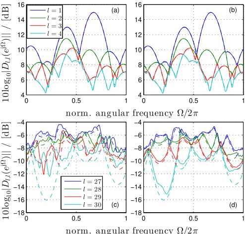
Experimental results for a single parahermitian matrix real-isation in Fig. 6, showing ground truth versus extracted eigen-values, exemplarily indicate that SMD prioritises resolution of eigenvalues with high power, and requires a high number of iterations to satisfactorily resolve eigenvalues with low power, while the DaC methods attempt to resolve all eigenvalues equally. This property of SMD has also been observed in [30]. For simplicity of the graphs in Fig. 6, only the strongest and weakest four of the30eigenvalues are shown, with the ground truth shown with dotted lines. A comparison of Fig. 6(a) and (b) indicates that SMD offers slightly better resolution of the first four eigenvalues, while Fig. 6(c) and (d) show that PSMD is more able to resolve the last four eigenvalues. More accurately resolving eigenvalues of low power may be advantageous when attempting to estimate the noise-only subspace in broadband angle of arrival scenarios, in which DaC techniques have already proved useful [22].
D. Mean Squared Error
The ensemble-averaged MSE of (20) for each algorithm forms column three of Tab. I. The DaC methods can be seen to introduce an error to the PEVD, and produce higher ensemble MSEs than SBR2 and SMD. By decreasing truncation levels, the MSE of all PEVD algorithms can be reduced at the expense of longer algorithm run-time and paraunitary matrices of higher order. Conversely, the higher truncation within PSMD1 has resulted in marginally higher MSE. To reduce the MSE of DCSMD, HDCSMD, and PSMD in this scenario,
IDcan be increased; however, this will reduce the speed of the algorithms, as more effort will be contributed to the ‘divide’ step. This can be observed in the results of PSMD2, which offers the lowest MSE of any of the tested algorithms.
0 0.5 1
4 6 8 10 12 14 16
0 0.5 1
4 6 8 10 12 14 16
1
0
lo
g10
|
Dl,
l
(
e
j
Ω)
||
/
[d
B
]
norm. angular frequencyΩ/2π
l= 1 l= 2 l= 3 l= 4
(b) (a)
0 0.5 1
−18 −16 −14 −12 −10 −8 −6 −4
0 0.5 1
−18 −16 −14 −12 −10 −8 −6 −4
1
0
lo
g10
|
Dl,
l
(
e
j
Ω)
||
/
[d
B
]
norm. angular frequencyΩ/2π
l= 27 l= 28 l= 29
l= 30 (c) (d)
Fig. 6. Ground truth (dashed) vs extracted (solid) (a,b) strongest and (c,d) weakest four polynomial eigenvalues obtained from (a,c) SMD and (b,d) PSMD when applied to a single instance of the specified scenario.
E. Paraunitarity Error
Ensemble averages for this error defined in (21) are listed in column four of Tab. I. Owing to their short run-time, low levels of truncation can be used for the DaC algorithms; this directly translates to low paraunitarity error. Conversely, high truncation is typically required to allow SBR2 and SMD to provide feasible run-times, resulting in higher η. The use of larger truncation parameters in PSMD1 has resulted in a significant increase in paraunitarity error, such that η is only slightly lower for PSMD1 than SMD. Increasing ID in PSMD2 has slightly increased η, as more iterations of the ‘divide’ step — and therefore more truncation operations — are completed.
F. Paraunitary Filter Length
Column five of Tab. I, showing the ensemble-average parau-nitary filter length of Sec. V-5, shows that DaC strategies tend to produce higher values for LF [22], [47], [52]. However, the use of compensated row-shift truncation in PSMD has resulted in lower LF. Using higher levels of truncation in any algorithm would reduce filter length and algorithm run-time at the expense of higher MSE andη; this relationship is observed in the results of PSMD1, which is able to provide significantly shorter paraunitary filters than PSMD. Indeed, the filters produced are actually shorter than those given by SMD. IncreasingID in PSMD2 has resulted in an increase inLF.
VII. ALGORITHMIMPLEMENTATION INHARDWARE
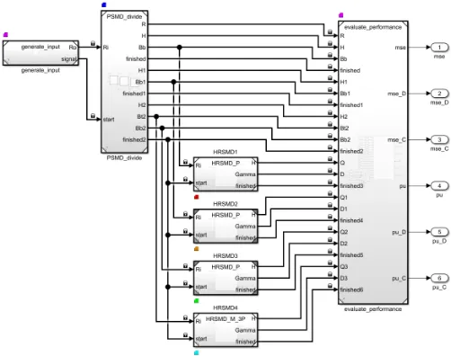
[image:10.612.313.560.55.291.2]Fig. 7. Model diagram of the parallel form of the algorithm implemented in SimulinkR.
The PSMD implementation is detailed in Sec. VII-A, while Secs. VII-B and VII-C discuss running this on a quad core CPU and Raspberry Pi, respectively, to highlight how paral-lelism is exploited.
A. Modular Realisation of Algorithm
When creating a block-based modular system implemen-tation, MATLABR’s Simulink and Embedded Coder can generate C code, but also provide various profiling tools, and enable the concurrent execution of tasks, depending on the target hardware platform. Since PSMD utilises multiple instances of the HRSMD and HRSMS algorithms, each of these instances can be formulated as a function block and subsequently allocated to a task.
In the model of Fig. 7, a first block generates a para-hermitian matrix according to Sec. VI-A. A ‘divide’ stage block hides three sequentially organised instances of HRSMS, followed by ‘conquer’ stage containing four parallel instances of HRSMD that diagonalise the four smaller parahermitian matrices. A last block provides access to result parameters for diagnostics.
If the C code generated by MATLABR’s Embedded Coder is compiled for deployment on hardware with a compatible operating system and multiple CPU cores, each of these tasks can be managed independently and can therefore be executed concurrently. The dovetailing of tasks may however introduce some additional latency, which can affect execution time. The latter will be influenced by the slowest block, which typically is the first instance of the HRSMS ‘divide’ stage operating on an M ×M matrix, while all other blocks operate on parahermitian matrices with smaller spatial dimension.
The parallel implementation of Fig. 7 can be contrasted by a serial implementation by forcing both the ‘divide’ and ‘conquer’ stages into a single block. For both serial and parallel implementations, some parameters must be preset. For memory conservation, parahermitian and paraunitary matrices are both limited to maximum lengths of 201, whereby the
(a) (b)
Fig. 8. Average execution time inµs for each task over 100instances of the (a) serial and (b) parallel implementation on an IntelR i7-4700MQ CPU. ‘System’ refers to model computations not associated with the algorithm.
half-matrix method conserves half the memory space for the parahermitian matrix. To keep memory use low, we have implemented PSMD1from Sec. VI-A, which permitted a
rel-atively high level of truncation and thus produced the shortest paraunitary matrices of all the considered DaC configurations.
B. Multicore CPU Implementation
For efficient implementation on an IntelR i7-4700MQ CPU, BLAS and LAPACK libraries were sourced via the IntelR Math Kernel Library. MATLABR, and therefore the simula-tion results of Sec. VI implicitly rely on these to facilitate fast matrix multiplication and useful EVD algorithms. Complex double precision was used throughout, therefore numerical accuracy was equivalent to results of Tab. I.
By segmenting the serial and parallel models into tasks, a profiler native to Simulink could be utilised to evaluate the timing performance of each task individually. Average performance was ascertained by running the models over 100 instantiations, with results for the task timings shown in Fig. 8(a) and (b) for the serial and parallel versions, respectively. For the serial version, the average execution time in Fig. 8(a) is 0.772 s. For the parallel version, each task represents one of the blocks in Fig. 7. The ‘divide’ stage takes on average 0.583 s to run; thereafter, the four ‘conquer’ stages operate in parallel. With the slowest HRSMD taking an average execution time of 0.079 s, the total average execution time for the parallel implementation is 0.663 s, thus about 16% faster than the serial implementation. Also note that parallelised and compiled version, while running on the same hardware as the results provided in Fig. 5, execute globally significantly faster than the MATLABR simulations of Sec. VI. Fig. 9 illustrates how each task is assigned a core at each sample time; the cores—four physical and four virtual ones—are numbered0-7.
[image:11.612.316.568.63.189.2]Fig. 9. Cores assigned to each task over the first30of100instances of the parallel implementation on an IntelR i7-4700MQ CPU.
TABLE II
AVERAGE RESOURCES UTILISED BY SERIAL AND PARALLEL
IMPLEMENTATIONS OF ALGORITHM ON ANINTELR I7-4700MQ CPU.
Model Execution time Memory usage Cores used
DCSMD 1.0846s 214709KiB 1
PSMD, serial 0.7717s 192883KiB 1
PSMD, parallel 0.6626s 192884KiB 5
C. Raspberry Pi Implementation
To demonstrate the implementation on a hardware device that is more stand-alone than the CPU in Sec. VII-B, we have targetted a Raspberry Pi 3B+ with a 1.4 GHz 64-bit quad-core ARM processor running a Mathworks-customised Linux operating system. With the same parahermitian matrix scenario as before, the models were compiled with a Simulink support package dedicated for this hardware. Standard Linux repositories provided the BLAS and LAPACK libraries for compilation. The models were downloaded to the Raspberry Pi 3B+ in the form of ‘.elf’ binary files; downloading as well as all other communication with the hardware platform were conducted via secure shell (SSH).
Due to unavailability of the profiling options reported in Sec. VII-A, Raspberry Pi 3B+’s CPU and memory usage were sampled with0.1s resolution using standard Linux commands; the results are shown for the serial model in Fig. 10. From the diagnostics of this graph, 100% of one CPU is dedicated to execution of the algorithm, while a further100%of a second CPU is used to generate the input parahermitian matrix and log the algorithm performance. The algorithm is the longer of the two processes; we see a step from 200% to 100% when the extraneous input/output process finishes. Algorithm completion occurs when the CPU utilisation drops to0%. We can therefore reliably measure the serial implementation by subtracting the start points from the end points. There is a baseload for the memory to hold the generated parahermitian matrix; spikes occur if processing additional resources is required.
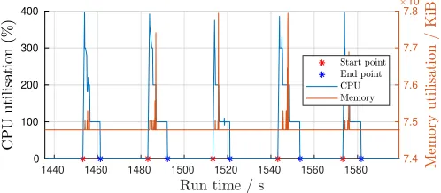
In the parallel results of Fig. 11, we see a large initial spike to 400% CPU utilisation, since the ‘divide’ stage (1 core), ‘conquer’ stage (2 cores), and input/output process (1 core) are pipelined and all executing simultaneously. The ‘conquer’ stage finishes first, dropping the CPU utilisation to 200%. The path from 200% → 100% → 0% is then the same as observed for the serial implementation. The memory usage of the parallel implementation is slightly higher compared to the serial one.
The resources of Tab. III were obtained following the
exe-1440 1460 1480 1500 1520 1540 1560 1580
0 50 100 150 200 250
7.4 7.5 7.6 7.7 7.8
[image:12.612.314.563.218.327.2]104
Fig. 10. CPU and memory utilisation over time of five instances of the serial model on a Raspberry Pi 3B+.
1440 1460 1480 1500 1520 1540 1560 1580
0 100 200 300 400
7.4 7.5 7.6 7.7 7.8 104
Fig. 11. CPU and memory utilisation over time of five instances of the parallel model on a Raspberry Pi 3B+.
TABLE III
AVERAGE RESOURCES UTILISED BY SERIAL AND PARALLEL
IMPLEMENTATIONS OF ALGORITHM ON ARASPBERRYPI3B+.
Model Execution time Memory usage Cores used
Serial 11.647s 74116KiB 1
Parallel 9.370s 74780KiB 3
cution of250instances of the serial and parallel models on the Raspberry Pi 3B+. By exploiting the parallel implementation that the PSMD algorithm’s structure affords, the execution time can be reduced by19.55%with only a minor increase in memory usage compared to a serial PSMD realisation. Note that the core count in Tab. III excludes the input/output blocks of the model; compared to the single-core operation of the serial model, the parallel model pipelines the ‘divide’ with the ‘conquer’ stage, where the latter are executed in parallel across two cores.
VIII. CONCLUSION
[image:12.612.333.543.406.442.2]When compared with the standard iterative SBR2 and SMD algorithms, PSMD offers a significant decrease in run-time and paraunitarity error — and provides superior eigenvalue resolution — but results in higher mean squared reconstruction error and paraunitary filter length. However, the latter can be reduced at the expense of higher paraunitarity error.
While the impact of DaC algorithm parameters Mˆ, P, and δ on performance metrics is not analysed here, research in [22] has investigated this topic for DCSMD and highlights the flexibility of this type of PEVD algorithm. Additional results in [47] demonstrate the increasing superiority of a DaC algorithm versus SMD when processing parahermitian matrices of increasing spatial dimension.
Two hardware implementations of the PSMD — one on an IntelR CPU, the other on a stand-alone Raspberry Pi — were demonstrated, and included the exploitation of symmetric structural features of a parahermitian matrix via the half-matrix method, and exploitation of parallelism through multi-core operation. This demonstrated enhanced execution time and memory use compared to an existing algorithm, and showed that the parallelism provides a significant improvement over a serial realisation.
When designing PEVD implementations for real appli-cations — particularly those involving a large number of sensors — the potential for the proposed method to increase diagonalisation speed while reducing complexity requirements offers benefits. In addition, the parallelisable nature of PSMD, which has been exploited here to reduce algorithm run-time, is well suited to hardware implementation.
For applications involving broadband angle-of-arrival es-timation, the short run-time of PSMD will decrease the time between estimations of source locations and bandwidths; similarly, use of PSMD will allow for signal of interest and interferer locations and bandwidths to be updated more quickly in broadband beamforming applications. Furthermore, the low paraunitarity error of PSMD, which facilitates the implementation of near-lossless filter banks, is advantageous for communications applications.
REFERENCES
[1] G. W. Stewart, “The decompositional approach to matrix computation,” Computing in Science Eng.,2(1):50–59, Jan. 2000.
[2] G. Golub and C. V. Loan,Matrix computations, 4th ed. Baltimore, ML: John Hopkins, 2013.
[3] I. Gohberg, P. Lancaster, and L. Rodman,Matrix Polynomials. New York: Academic Press, 1982.
[4] P. P. Vaidyanathan, Multirate Systems and Filter Banks. Englewood Cliffs: Prentice Hall, 1993.
[5] J. G. McWhirter, P. D. Baxter, T. Cooper, S. Redif, and J. Foster, “An EVD Algorithm for Para-Hermitian Polynomial Matrices,”IEEE TSP, 55(5):2158–2169, May 2007.
[6] S. Icart and P. Comon, “Some properties of Laurent polynomial matri-ces,” inIMA Int. Conf. Math. Signal Proc., Dec. 2012.
[7] P. P. Vaidyanathan, “Theory of optimal orthonormal subband coders,” IEEE TSP,46(6):1528–1543, June 1998.
[8] S. Weiss, J. Pestana, and I. K. Proudler, “On the existence and unique-ness of the eigenvalue decomposition of a parahermitian matrix,”IEEE TSP,66(10):2659–2672, May 2018.
[9] S. Weiss, J. Pestana, I. Proudler, and F. Coutts, “Corrections to on the existence and uniqueness of the eigenvalue decomposition of a parahermitian matrix,”IEEE Transactions on Signal Processing, vol. 66, no. 23, pp. 6325–6327, Dec. 2018.
[10] C. Delaosa, F. K. Coutts, J. Pestana, and S. Weiss, “Impact of space-time covariance estimation errors on a parahermitian matrix evd,” in IEEE SAM, Sheffield, UK, July 2018.
[11] C. H. Ta and S. Weiss, “A design of precoding and equalisation for broadband MIMO systems,” in Asilomar Conf. SSC, pp. 1616–1620, Nov. 2007.
[12] R. Brandt and M. Bengtsson, “Wideband MIMO channel diagonalization in the time domain,” inPIMRC, pp. 1958–1962, Sept. 2011.
[13] N. Moret, A. Tonello, and S. Weiss, “MIMO precoding for filter bank modulation systems based on PSVD,” inProc. IEEE 73rd VTC, pp. 1–5, May 2011.
[14] A. Sandmann, A. Ahrens, and S. Lochmann, “Resource allocation in svd-assisted optical mimo systems using polynomial matrix factoriza-tion,” inITG Symp. Photonic Networks, May 2015.
[15] A. Sandmann, A. Ahrens, and S. Lochmann, “Performance analysis of polynomial matrix SVD-based broadband mimo systems,” inSSPD, Edinburgh, UK, Sep. 2015.
[16] A. Ahrens, A. Sandmann, E. Auer, and S. Lochmann, “Optimal power allocation in zero-forcing assisted PMSVD-based optical MIMO sys-tems,” inSSPD, Edinburgh, UK, Dec. 2017.
[17] C. H. Ta and S. Weiss, “A jointly optimal precoder and block decision feedback equaliser design with low redundancy,” inEUSIPCO, Poznan, Poland, pp. 489–492, Sep. 2007.
[18] J. Foster, J. G. McWhirter, S. Lambotharan, I. K. Proudler, M. Davies, and J. Chambers, “Polynomial matrix QR decomposition for the decod-ing of frequency selective multiple-input multiple-output communication channels,”IET Signal Proc.,6(7):704–712, Sep. 2012.
[19] S. Weiss, M. Alrmah, S. Lambotharan, J. McWhirter, and M. Kaveh, “Broadband angle of arrival estimation methods in a polynomial matrix decomposition framework,” inIEEE CAMSAP, pp. 109–112, Dec. 2013. [20] M. Alrmah, S. Weiss, and S. Lambotharan, “An extension of the music algorithm to broadband scenarios using polynomial eigenvalue decomposition,” inEUSIPCO, pp. 629–633, Aug. 2011.
[21] M. Alrmah, J. Corr, A. Alzin, K. Thompson, and S. Weiss, “Polynomial subspace decomposition for broadband angle of arrival estimation,” in SSPD, Sep. 2014.
[22] F. K. Coutts, K. Thompson, S. Weiss, and I. Proudler, “Impact of fast-converging PEVD algorithms on broadband AoA estimation,” inSSPD, Dec. 2017.
[23] S. Redif, J. G. McWhirter, P. D. Baxter, and T. Cooper, “Robust broadband adaptive beamforming via polynomial eigenvalues,” inProc. IEEE/MTS OCEANS, Sep. 2006.
[24] S. Weiss, S. Bendoukha, A. Alzin, F. Coutts, I. Proudler, and J. Cham-bers, “MVDR broadband beamforming using polynomial matrix tech-niques,” inEUSIPCO, pp. 839–843, Sep. 2015.
[25] A. Alzin, F. Coutts, J. Corr, S. Weiss, I. K. Proudler, and J. A. Chambers, “Adaptive broadband beamforming with arbitrary array geometry,” in IET/EURASIP ISP, Dec. 2015.
[26] S. Redif, J. McWhirter, and S. Weiss, “Design of FIR paraunitary filter banks for subband coding using a polynomial eigenvalue decomposi-tion,”IEEE TSP,59(11):5253–5264, Nov. 2011.
[27] S. Weiss, S. Redif, T. Cooper, C. Liu, P. D. Baxter, and J. G. McWhirter, “Paraunitary oversampled filter bank design for channel coding,”EURASIP J. Adv. Sig. Proc., Mar. 2006.
[28] S. Redif, S. Weiss, and J. McWhirter, “Relevance of polynomial ma-trix decompositions to broadband blind signal separation,” Sig. Proc., 134:76–86, May 2017.
[29] S. Weiss, N. J. Goddard, S. Somasundaram, I. K. Proudler, and P. A. Naylor, “Identification of broadband source-array responses from sensor second order statistics,” inSSPD, London, UK, Dec. 2017.
[30] S. Redif, S. Weiss, and J. McWhirter, “Sequential matrix diagonalization algorithms for polynomial EVD of parahermitian matrices,”IEEE TSP, 63(1):81–89, Jan. 2015.
[31] J. Corr, K. Thompson, S. Weiss, J. McWhirter, S. Redif, and I. Proudler, “Multiple shift maximum element sequential matrix diagonalisation for parahermitian matrices,” inIEEE SSP, pp. 312–315, June 2014. [32] Z. Wang, J. G. McWhirter, J. Corr, and S. Weiss, “Multiple shift second
order sequential best rotation algorithm for polynomial matrix EVD,” in EUSIPCO, pp. 844–848, Sep. 2015.
[33] J. Corr, K. Thompson, S. Weiss, J. G. McWhirter, and I. K. Proudler, “Causality-Constrained multiple shift sequential matrix diagonalisation for parahermitian matrices,” inEUSIPCO, pp. 1277–1281, Sep. 2014. [34] A. Tkacenko and P. Vaidyanathan, “Iterative greedy algorithm for
![Fig. 1. Concept of PSMD: (a) original matrix Rapplied to each subblock separately leads to (c) the diagonalised output[τ] ∈ C20×20, which in afirst ‘divide’ paraunitary similarity transform step yields (b) the block diagonalresult R′[τ]; a second paraunitary similarity transform, which can now be D[τ].](https://thumb-us.123doks.com/thumbv2/123dok_us/1334582.87246/4.612.311.564.54.129/separately-diagonalised-paraunitary-similarity-diagonalresult-paraunitary-similarity-transform.webp)

![Fig. 5. Performance of PSMD, PSMD1SMD [30], DCSMD [52], and half-matrix DCSMD for the decomposition ofa, and PSMD2 relative to SBR2 [5], 30 × 30 parahermitian matrix.](https://thumb-us.123doks.com/thumbv2/123dok_us/1334582.87246/9.612.315.562.61.151/performance-dcsmd-matrix-dcsmd-decomposition-relative-parahermitian-matrix.webp)