Robust optimisation of low-thrust interplanetary transfers using evidence theory

AAS 19-285

ROBUST OPTIMISATION OF LOW-THRUST INTERPLANETARY

TRANSFERS USING EVIDENCE THEORY

Marilena Di Carlo

_{, Massimiliano Vasile}

_{, C. Greco}

_{and R. Epenoy}

This work presents the formulation and solution of optimal control problems under epistemic uncertainty, when this uncertainty is modelled with Dempster-Shaffer theory of evidence. The application is to the design of low-thrust interplanetary transfers when an epistemic un-certainty exists in the performance of the propulsion system and in the magnitude of the departure hyperbolic excess velocity. The problem is solved by transforming the exact for-mulation, that uses discontinuous Belief functions, into an inexact formulation that uses a new continuous statistical function, calledS in the following, that approximates the value

of the Belief function. The optimisation is realised by first building a surrogate model of the quantities of interest and associatedSfunctions. The surrogate is then progressively

up-dated as the optimisation proceeds. The proposed method is applied to the design of optimal low-thrust transfers from the Earth to asteroid Apophis.

INTRODUCTION

In the early phases of the design of a space mission, the values of several design parameters are either unknown or are known with a degree of uncertainty.1 _{An insufficient consideration for uncertainty, in this}

phase, would lead to a wrong decision on the feasibility of the mission.2 _{In this work, uncertainty}

quantifi-cation is applied to the optimisation of low-thrust interplanetary trajectories. In particular, the optimisation under uncertainty is realised making use of the Dempster-Shaffer theory of evidence,3 _{for the case when}

epistemic uncertainty exists in the system parameters of the low-thrust spacecraft (thrust and specific impulse of the engine) and in the magnitude of the departure hyperbolic excess velocity. The considered problem is a low-thrust transfer from Earth to asteroid Apophis.

The paper is organised as follow. The first two sections introduce the theoretical background required for the formulation of the problem of optimisation under uncertainty. In particular, at first, Uncertainty Quantification using Evidence Theory is presented; then, the Low-Thrust Transfer Optimal Control Problem is described. The problem of Optimisation under Uncertainty is then introduced. The case study and the results of the proposed method are then presented for the Earth-Apophis transfer.

UNCERTAINTY QUANTIFICATION USING EVIDENCE THEORY

Evidence Theory, or Dempster-Shaffer theory, belongs to the class of imprecise probability theories devel-oped to treat both epistemic and aleatory uncertainty, when no information about the probability distribution is available.4 _{In Evidence Theory, uncertainties are defined by means of Basic Probability Assignments}

(BP A), associated to elementary propositionsAin the space of possible eventsΘ. BeingΘthe set of all

∗_{Research Associate, Department of Mechanical and Aerospace Engineering, University of Strathclyde, 75 Montrose Street, G1 1XJ,}

Glasgow, United Kingdom.

†_{Professor, Department of Mechanical and Aerospace Engineering, University of Strathclyde, 75 Montrose Street, G1 1XJ, Glasgow,}

United Kingdom

‡_{PhD Student, Department of Mechanical and Aerospace Engineering, University of Strathclyde, 75 Montrose Street, G1 1XJ, Glasgow,}

United Kingdom

possibilities, the Basic Probability Assignment is a functionBP A: 2Θ_{→[0,1]verifying}

BP A(∅) = 0,

X

A⊂Θ

BP A(A) = 1. (1)

In model-based systems engineering, elementary propositions will often take the form of an uncertain quantity

ξbeing within a set of intervals, i.e.

A={ξ∈[al, bl]}, 1≤l≤ L, (2)

and their associatedBP A. In Equation (2),Lis the number of intervals[al, bl]associated to the quantity

ξ. Note thatBP Acan be associated to potentially overlapping or disjoint intervals as well as to their union,

the latter representing a degree of ignorance. If several uncertain variables are taken into account, one will consider propositions of the kind

A={ξ= (ξ1, ξ2,· · ·, ξnξ)∈

nξ

Y

j=1

[aj,lj, bj,lj] =Hl}, 1≤lj≤ Lj, (3)

wherenξ is the number of uncertain variables and[aj,lj, bj,lj]denote the bounds of thelj-th interval of the

j-th variables. In Equation (3),l= (l1, l2,· · ·, lnξ)is the multivariate index associated to hyperrectangular

domainHl. Assuming independent uncertainties, theBP Aof every such possibility can be computed as the

product of theBP Aof the elementary propositions regarding eachξj,

BP A(Hl) =

nξ

Y

j=1

BP Aj,lj , (4)

whereBP Aj,lj is the BPA associated to the interval lj of the uncertain variablej. After combination of

several, possibly conflicting, evidence sources,5–7_{a map of probability masses is thus assigned to all elements}

in2Θ_{. The Belief (Bel) on and Plausibility (P l) of a given propositionA⊆Θare defined as}

Bel(A) = X B|B⊆A

BP A(B),

P l(A) = X B|B∩A6=∅

BP A(B), (5)

i.e. Bel(A)collects the BPA associated to possibilitiesBsatisfyingA, whereasP l(A)collects the BPA of possibilitiesBnot contradictingA. Hence

P l(A) = 1−Bel( ¯A), (6)

and Belief and Plausibility can be interpreted as the lower and upper bounds, respectively, imposed by the evi-dence available on the imprecise probabilityP(A). The difference betweenP l(A)andBel(A)constitutes an indicator of the degree of second-order uncertainty associated to the assessment ofP(A). This interpretation

is illustrated in Figure 1.

In the applications that concern this work, the formulation presented translates into considering a mapping ofBP Aover a family of hyperrectangular subsets Hl of the space of uncertain variables. This family of

subsets is referred to asΞ, the uncertainty space, and needs to contain every focal elementθ, that is every subset ofΘwith non-nullBP A:

Ξ⊇[θ , θ⊂Θ, BP A(θ)>0. (7)

TheBP Astructure ofΞ can then be used to calculate the lower (Belief) and upper (Plausibility) bounds on the probability that the value of a quantity of interestJ(ξ)is as expected, e.g. under a thresholdν, by

considering

A={ξ∈Ξ|J(ξ)≤ν}, (8) which gives

Bel(J(ξ)≤ν) =X θ

BP A(θ),

P l(J(ξ)≤ν) =X θ

BP A(θ), (9)

with

θ={θ⊂Θ| max

ξ∈Hl⊆θ

(J(ξ))≤ν},

θ={θ⊂Θ| min

ξ∈Hl⊆θ(F(ξ))≤ν}.

(10)

Thus, in robust design optimisation, the robustness of a design against the epistemic uncertainty in the system is usually characterised by the curvesBel(J(ξ) ≤ ν)andP l(J(ξ) ≤ ν)againstν associated to that design – henceforth referred to simply as Belief and Plausibility curves. In particular, if J is to be minimised, thenA as defined above is the desirable hypothesis, and the robustness index is often chosen asBel(J(ξ) ≤ ν)since it can be interpreted as a conservative estimation of the probability associated to the desirable hypothesis. The drawback of this comprehensive approach for uncertainty quantification is that it leads to an NP-hard problem with a computational complexity that is exponential with the number of epistemic uncertain variables. This is due to the fact that a global maximisation (or minimisation) of the quantity of interest is required over eachθ ⊂ Ξhaving non-null BP A(Equation (10)). In this work

this issue is tackled using surrogate models of the quantities of interest, in order to reduce the computa-tional time associated to the minimisation and maximisation. The single objective optimisation problems given in Equations (10) are solved using Multi-Population Adaptive Inflationary Differential Evolution Al-gorithm (MP-AIDEA),8_{an adaptive multi-population evolutionary algorithm based on the hybridisation of}

Differential Evolution with Monotonic Basin Hopping. MP-AIDEA is available open-source on GitHub at

https://github.com/strath-ace/smart-o2c/tree/master/Optimisation.

LOW-THRUST TRANSFER OPTIMAL CONTROL PROBLEM

The use of Evidence Theory to treat uncertainties is applied to the optimal control problem of an interplan-etary low-thrust transfer. The low-thrust optimal control problem is transcribed with a variant of the direct analytical shooting algorithm proposed by Zuiani et al.9_{and implemented in the software code FABLE (FAst}

Boundary-value Low-thrust Estimator).10 _{The code FABLE is available open source on GitHub athttps:}

//github.com/strath-ace/smart-o2c/tree/development/Transcription/FABLE. The

idea of this transcription method is to split the trajectory into a predefined sequence ofnLT finite coast and thrust arcs. Eachs-th thrust arc is represented by the low-thrust acceleration components, ar, atandah expressed in a local radial-transverse-normal reference frame as:9

aLT,s=  



ar

at

ah  

 s

=  



scosαscosβs

ssinαscosβs

ssinβs  



whereαsandβsare, respectively, the azimuth and elevation angles andsis the modulus of the acceleration:

s=

F ms

1

(r/r¯)2 . (12)

In Equation (12),Fis the thrust of the engine,msis the mass of the spacecraft on thes-th arc, and¯r= 1AU. The trajectory is analytically propagated from the departure point to the arrival point. The departure state is defined by the state of the Earth on the departure day; the departure velocity vector is obtained considering both the velocity of the Earth and the departure hyperbolic excess velocity vectorv∞, defined, in an

Earth-centered reference system, as:

v∞= [v∞cosαcosδ, v∞sinαcosδ, v∞sinδ]T . (13)

In Equation (13),αandδare the departure azimuth and declination angles. The arrival state is defined by the state of the target body on the arrival day, considering a two-body dynamics. The motion of the spacecraft is assumed purely Keplerian along coast arcs while thrust arcs are analytically propagated using an asymptotic expansion solution based on the work of Zuiani and Vasile.11 _{Each arc begins and ends at anOn/Of f}

control node, whereOnnodes define the switching point from a coast to a thrust arc andOf f nodes define

the switching point from a thrust to a coast arc. The azimuth and elevation angles,αsandβs, are constant along a thrust arc, whileschanges according to Equation (12). The optimisable vector for each transfer is defined by the anglesαsandβsfor each thrust arc, by the true longitude of theOn/Of f control nodes, and by the azimuth and declination angles at lunch (the magnitudev∞is assumed to be known):

u= [L1,On, L1,Of f, α1, β1, L2,On, L2,Of f, α2, β2, . . . LnLT,On, LnLT,Of f, αnLT, βnLT, α, δ]

T _{. (14)}

The objective function of the optimal control problem is the total∆V, calculated as:

J(u, v∞, F, Isp) = ∆V =

nLT

X

s=1 Z

sdt=

Z _Fr¯2

r(t)2_m(t)dt . (15)

In the conservative assumption thatmstays constant on each thrust arc, the integrals for the computation of ∆V can be transformed into integrals in the true longitudeL, that can be solved analytically to give:

J(u, v∞, F, Isp) = ∆V ≈

nLT

X

s=1

F ¯r2

ms

1 p

µas(1−e2 s)

∆Ls, (16)

whereas,esandmsare, respectively, the semi-major axis, eccentricity and mass at the beginning of thes-th thrust arc, and∆Ls = Ls,Of f −Ls,Onis the variation of the true longitude on the thrust arc. The values ofasandes, fors = 1, depend uponv∞; the massmsis updated at the end of each thrust arc using the considered value of the specific impulse, according to:

ms+1=ms−

F

p

µas(1−e2 s)

∆Ls

Ispg0

. (17)

The analytical expression in Equation (16) is obtained from Equation (15) using:9

dt dL =

s

a3

µ

(1−e2₎3 (1 +P1sinL+P2cosL)

2 (18)

and

r(L) = a(1−e 2₎

(1 +P1sinL+P2cosL)

, (19)

(18) is an approximated expression that does not include the direct effect of the thrust on the variation ofL. This approximation provides acceptable results for control acceleration levels that are typical of existing low-thrust propulsion systems. The use of the analytical expression forJspeeds up the optimisation process with respect to the use of a numerical integration, while still giving accurate results. The non-linear programming problem to solve is:

min

u∈UJ(u, v∞, F, Isp) s.t. xf inal= ¯xf

PnLT

s=1∆ts=T oF

(20)

wherexf inalis the final state of the spacecraft at the end of the propagation,x¯f is the desired arrival state andT oF is the desired time of flight. The non-linear programming problem is solved using the MatlabR fmincon-interior-pointalgorithm.

OPTIMISATION UNDER UNCERTAINTY

The previous two sections have presented the formulation of the uncertainty quantification using Evidence Theory and the formulation of the low-thrust transfer optimal control problem. These two concepts will be now combined to define the problem of optimisation under uncertainty of a low-thrust transfer, using Evidence Theory. The problem is formulated as follows:

max

u∈U Bel(J(x,u,ξ)∈Ψ) s.t. x˙ =f(x,u,ξ, t)

g(x,u,ξ, t)≥0

Bel(ψ(x0,xf(ξ), t0, tf)∈Φ)>1−ε

t∈[t0, tf]

(21)

wherex∈ Rn_{is the state vector,uthe control vector,ξthe uncertainty vector of dimensionnξ,tthe time,}

f the dynamic of the system,ψthe function defining the final state of the system andΦthe target set. The subscripts0andfdenote initial and final conditions, respectively. The goal is to maximize the beliefBel, or lower probability, that the cost functionJ belongs to the setΨ, with the beliefBelof constraint satisfaction being greater than a given positive value1−ε.

In the following, Problem (22) will be specifically written and expressed for the case of a low-thrust transfer. In this case, the optimal control problem under uncertainty is formulated as:

max

u∈U Bel(mprop≤ν¯mprop) s.t. x˙ =f(x,u,ξ, t)

Bel(∆r≤ν¯∆r)>1−ε∆r

Bel(∆v≤ν¯∆v)>1−ε∆v

(22)

The goal is to find the controlu, in the space of the controlsU, that maximise the beliefBelthat the mass of propellantmpropis lower or equal than a thresholdν¯mprop. At the same time, the control must satisfy some

position and velocity constraints expressed in terms of the Belief function. In particular, given the thresholds ¯

ν∆randν¯∆vfor the position and the velocity constraint violations∆rand∆v, it is required for the Belief of ∆r≤¯ν∆rand the Belief of∆v≤ν¯∆vto be greater than1−∆rand1−∆v, respectively.

The solution of Problem (22) presents some difficulties, from a computational point of view. In particular:

• the computation of the Belief function for each control urequires the solution of a maximisation

problem,2_{over all the focal elements of the uncertainty space;}

• the function Bel is discontinuous and cannot be easily represented with a surrogate model. On the other hand, the availability of a surrogate forBelwould avoid the need to realise the maximisation of the quantities of interest over all the focal elements, and for each new control vector (a procedure that is required to compute the Belief).

In this paper, these challenges are addressed with a combination of the following techniques:

• surrogate models of the quantities of interest,mprop,∆rand∆v, are used to speed up the maximisation

over each focal element, for each control vectoru; these surrogate models will be called “internal” in

the following, and will be denoted with the symbolsm˜prop,∆frand∆fv;

• given that the uncertainty space Ξis smaller than the control space U, a dimensionality reduction

method is devised so that Problem (22) can be solved over the space of the uncertain parametersΞ, rather than the space of the controlsU;

• surrogate models are used to represent a continuous approximation of theBel function, so that the optimisation of Problem (22) can be realised on a continuous surrogate model of the continuous ap-proximation ofBel. The continuous approximation ofBelwill be calledS in the following, and its

surrogate_S˜_{will be called “external” surrogate.}

By using these three techniques, Problem (22) can be formulated as:

max

ξ∈Ξ ˜

S( ˜mprop≤ν¯mprop)

s.t. _S˜ f ∆r≤ν¯∆r

>1−ε∆r,S ˜

S∆fv≤ν¯∆v

>1−ε∆v,S

(23)

The variables ε∆r,S andε∆r,S in Problem 23 are related to the variables ε∆r andε∆r of Problem (22). A detailed explanation of the relationship betweenε∆r,S andε∆r,S andε∆r andε∆rwilll be given in the following. The next subsections will give more details about the correspondence between Ξ andU, the

internal and external surrogate models, and the functionS.

Dimensionality Reduction and Mapping BetweenΞandU

In this work it is assumed that for a given uncertain vector¯_{ξthere is one and only one controlu¯ that is} globally optimising the quantity of interest and satisfying the constraints. This implies that we can define a one-to-one functional relationship between the space of the feasible and global optima controlsU and the

space of the uncertain parametersΞ. This one-to-one correspondence can be used to replace the optimisation vectoruwith the smaller dimensional optimisation vectorξ. The functional relationship can be recovered

through the solution of Problem (20). In fact, for a given value of_ξ¯_{, and using Equations (33) to (35),}¯_ξwill be uniquely associated to a vector of controlsu¯. The criticality of this dimensionality reduction approach is the identification of the feasible and global optimal control law. Although this identification is theoretically possible, it is also practically challenging. On the other hand, one can accept also the identification of a local minimum, as long as local minima are unique, because local minima correspond to conservative solution of the proposition(mprop≤ν¯mprop), for which theBelneeds to be maximised. While in this paper the analysis

is restricted to the space of the feasible and optimal controls, future work will be devoted to extend the study to the space of all the control laws, including the non feasible and non optimal ones.

Internal Surrogate Models

1. A surrogate model for the propellant mass, for different values of the uncertainty vectorξ, and for a fixed value of the control vectoru¯:

˜

mprop(ξ,u¯)≈mprop(ξ,u¯) ξ∈Ξ (24) The surrogate model m˜prop describes how the mass of propellant required to realise the transfer changes when the system parameters are different from_ξ¯_{, but the control is kept equal tou¯.}

2. A surrogate model for the violation of the final constraints on the position:

f

∆r(ξ,u¯)≈∆r(ξ,u¯) ξ∈Ξ (25)

The surrogate model ∆fr describes how the final violation of the constraint on the position changes when the system parameters are different from¯_{ξ, but the control is kept equal to the controlu¯.} 3. A surrogate model for the violation of the final constraints on the velocity:

f

∆v(ξ,u¯)≈∆v(ξ,u¯) ξ∈Ξ (26)

The responses of the training points used to build the surrogate models,T =

ξp Np

p=1, are obtained prop-agating the dynamic equations for the motion of the spacecraft using the nominal controlu¯ and different values of the uncertainty vectorξ. For a given controlu¯ and set of uncertain parametersξ, the state vector x= [r,v, m]T of the spacecraft at timetfis computed as:

x(ξ,u¯, tf) = [r(ξ,u¯, tf),v(ξ,u¯, tf), m(ξ,u¯, tf)]T =x0+ Z tf

t0

f(x,u¯,ξ, t)dt . (27)

The integration in Equation (27) is performed analytically, using a first order expansion in the perturbing acceleration.11 _{The responses of the training points for the three surrogate models are computed as:}

mprop=m0−m(ξ,u¯, tf) ∆r=kr(ξ,u¯, tf)−rtargetk ∆v=kv(ξ,u¯, tf)−vtargetk,

(28)

wherem0is the initial mass of the spacecraft at launch, andrtargetandvtargetare the targeted position and velocity vectors. The use of the surrogate models replace, therefore, the propagation in Equation (27) with the evaluation of the surrogate functions. The surrogate models are generated from the training pointsT, and

the correspondingmprop,∆rand∆vcomputed through Equation (28), using the Matlab toolbox DACE.12

The SmoothBel/P lFunction

The use of the internal surrogate models speeds up the computation of the Belief. This makes the com-putation of the Belief associated to a single uncertain vector¯_{ξand corresponding controlu¯ relatively fast,} but the computation is still not fast enough for the evaluations of the function at several points, as required by the solution of Problem (22). The solution of Problems (22) requires, in fact, an optimisation process that has to evaluate theBelat several pointsξ. To solve this difficulty, surrogate models of the functions Bel(mprop≤ν¯mprop),Bel(∆r≤¯ν∆r)andBel(∆v≤¯ν∆v)could be built, so as to speed up the

optimisa-tion. These surrogate models are denoted as “external”. However, the Belief is a discontinuous function, and it is difficult to create the surrogate model of a discontinuous function. To avoid the problems associated with the creation of the surrogate model of the Belief, and with the optimisation of a discontinuous function, the Belief is substituted by a continuous function. The external surrogate models are then built for the continuous function that substitutes the Belief, rather than for the Belief itself. The continuous function that substitutes the Belief, denoted asS, is referred to as “SmoothBel/P lfunction”. The functionSis defined as:

S(J(ξ)≤ν) =X θ∈Θ

BP A(θ) R

θ1(J(ξ)≤ν)dξ

Vθ

k

whereVθis the hypervolume of the focal elementθand1is the indicator function. Due to the normalisation of the integral at the numerator of Equation 29 withVθ, the term in square brackets will assume only values in the range[0,1]. The integral in Equation (29) is computed by sampling each focal elementθat a given number of points, and then numerically integrating, via Monte Carlo integration, a function that assumes values equal to 1 at the sampling points where the inequalities are satisfied, and 0 at the sampling points where the inequalities are not satisfied. Figure 2 shows a graphical representation of the computation of the integral in the functionS, for a one-dimensional example with two focal elements,F E1andF E2, characterised by

BP A1andBP A2. In particular, with reference to Figure 2:

Figure 2: Graphical representation for the computation of the integral in Equation (29).

Bel=BP A1

P l=BP A1+BP A2

S=BP A1·1k+BP A2·0.5k

(30)

and therefore

Bel≤S≤P l . (31)

The functionScoincides withBelandP lwhenk → ∞andk= 0, respectively. The Belief, Plausibility and functionS, for different values ofk, are represented in Figure 3 for a given controluˆ. Figure 3 shows thatSis alwaysBel≤S≤P l.

38 40 42 44 46 48 50 52 0

0.2 0.4 0.6 0.8 1

Bel / Pl / S

Bel Pl S k=0.1 S k=0.5 S k=1 S k=10 S k=100

Figure 3:Bel,P landScurves for the mass of propellant.

In the new formulation of Problem (22), introduced in Equation (23), the objective functionBel(mprop≤ ¯

Bel(∆r≤ν¯∆r)andBel(∆v≤ν¯∆r)are substituted bySe∆r ≈S∆r=S(∆r≤ν¯∆r)andSe∆v ≈S∆v =

S(∆v ≤ν¯∆v), respectively. Finally, by performing the optimisation in the spaceΞrather thanU, Problem (22) becomes:

max

ξ∈Ξ Semprop

s.t. Se∆r>1−ε∆r,S

e

S∆v>1−ε∆v,S

(32)

which is equivalent to Problem (23). In Problem (32), the quantitiesε∆r,S andε∆v,S must satisfyε∆r,S ≤

ε∆randε∆v,S ≤ ε∆v, whereε∆r andε∆v have been defined in Problem (22). The values of∆r,S and

∆v,S are obtained from an iterative process that starts from0∆r,S = ∆r and0∆v,S = ∆v and proceed by decreasing∆r,S and∆v,S at each step. This iteration process is necessary because of the property of functionS of being alwaysS ≥Bel (Figure 3); as a consequence, a pointξsatisfyingBel∆r > 1−∆r andBel∆v > 1−∆v might not satisfyS∆r > 1−∆randS∆v > 1−∆v. The iterations stop when

values of∆r,S and∆v,sare reached such that whenBel∆r >1−∆ralsoS∆r >1−∆r,S, and when

Bel∆v >1−∆valsoS∆v>1−∆v,S.

Summary of the Proposed Solution Method

The diagram flows in Figures 4 and 5 summarise the proposed solution method for the optimal control problem under uncertainty. The first step is the generation ofN training points in the uncertaint spaceΞ (Figure 4); these are defined using an Halton sequence. Each one of the training points is evaluated using the method described in Figure 5, in order to obtain the corresponding values of theBelandS functions. The

values of these functions, for all the training points, are then collected, and DACE is used to generate the external surrogate models_S˜_{. UsingS}˜_{, Problem (32) is solved, making use of the algorithm MP-AIDEA. The} optimal uncertain vectorξopt, solution of Problem (32), is evaluated using the method described in Figure 5. The new value ofScorresponding toξoptis used to update the external surrogate models. The process stops when the maximum number of iterations is reached. The iterative process allows to update the external surrogate models after each optimisation, so that accurate surrogate models can be locally obtained in the region where the solutions of the problem are located. The evaluation ofBel andS for a single point ξ

follows the method described in Figure 5. The first step is the solution of the NLP problem corresponding to Problem (20), for the given vector of uncertain parameters_ξ¯_{. As already mentioned, the solution of the} NLP problem provides a solution vector which uniquely identifies a vector of controlu¯. Usingu¯, the internal surrogate models can be computed, from which the values ofBelandScan then be obtained.

CASE STUDY: EARTH-APOPHIS LOW-THRUST TRANSFER

The computational framework described in this paper is applied to the design of a simple low-thrust trajec-tory from the Earth to asteroid Apophis. The considered transfer starts on 22 October 2026. The arrival date at Apophis is 11 July 2028. The orbital elements for the asteroid Apophis, for the epoch 24 September 2008, are taken from the JPL Small-Body Database∗_{. The state of Apophis at the arrival date 11 July 2028,x¯}

f, is then computed considering a Keplerian motion around the Sun. The mass of the spacecraft at departure is 644.3 kg. This section will introduce the considered vector of uncertaint parameters, the nominal trajectory, and the results of the optimisation under uncertainty.

Uncertain Parameters

The considered uncertain parameters are the magnitudev∞ of the departure hyperbolic excess velocity

vector, and the values of the thrustF and specific impulseIspof the engine during the transfer. In particular, it is assumed that the thrust and the specific impulse are subject to an uncertainty that is linearly dependent on the position of the spacecraft along its trajectory (denoted by the true longitudeL):

Start

DefineN train-ing pointsξi inΞ

ComputeBel

andS for ξi

Create external surrogate models_S˜

Solve Problem (32) to obtainξopt

ComputeBel

andS for ξopt

Max. n of iterations reached?

End

Update external surrogate models_S˜

yes no

Figure 4: Summary of the proposed solution method for the solution of the optimal control problem under uncertainty.

Solve NLP prob-lem (Probprob-lem (20)) for a given¯_ξ

Getu¯ corre-sponding to¯_ξ

Create internal surro-gate models using u¯

ComputeBeland S using the internal

surrogate models

Figure 5: Computation ofBelandScorresponding to a vector_ξ¯_{of uncertain parameters.}

The variablesF1,F2andIsp1,Isp2can be expressed using the values of the thrust and specific impulse at the initial and final true longitudes of the transfer,L0andLf:

FL0 =F(L0) =F1+F2L0, Isp,L0 =Isp(L0) =Isp1+Isp2L0,

FLf =F(Lf) =F1+F Lf, Isp,Lf =Isp(Lf) =Isp1+Isp2Lf .

The quantitiesF1,F2,Isp1andIsp2can be derived fromFL0,FLf,Isp,L0andIsp,Lf using:

F1=

FL0Lf−FLfL0

Lf−L0

,

F2= FLf −FL0 Lf−L0

.

(35)

The vector of uncertain variables includes, therefore, five parameters: ξ=

v∞, FL0, FLf, Isp,L0, Isp,Lf

T . The range for the uncertain parameters is reported in Table 1, whereξLdenotes the lower bound andξU the upper bound.

Table 1: Uncertainty range of the uncertain parameters.

v∞[km/s] Isp,L0[s] Isp,Lf [s] FL0 [N] FLf [N]

ξL 3 2772 2772 0.0477 0.0477

ξU 3.7 3388 3388 0.0583 0.0583

Nominal Trajectory

The nominal values of the system parameters are reported in Table 2. The nominal low-thrust optimisation

Table 2: Nominal values of the system parameters.

v∞[km/s] Isp,L0[s] Isp,Lf [s] FL0 [N] FLf [N]

Nominal 3.34 3080 3080 0.053 0.053

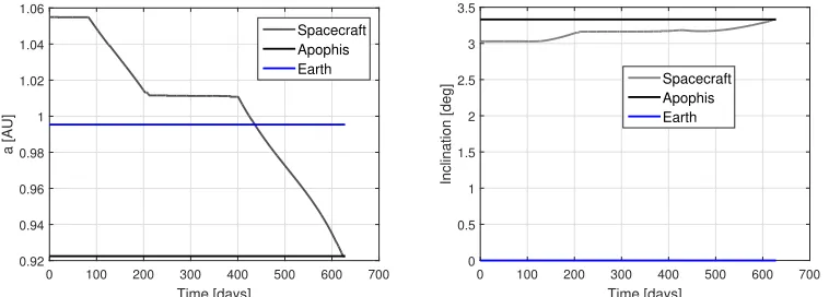
problem is solved using the solution method described in the Section titled “Low-Thrust Transfer Optimal Control Problem”. Figure 6 shows the projection in thex-yplane of the trajectory of the spacecraft and the distance of the spacecraft from the Sun during the transfer; coast arcs are represented in green and thrust arcs in red. Figure 7 shows the variation of semi-major axis and inclination of the spacecraft during the transfer. The ∆V of the transfer is 2.1584 km/s, corresponding to a propellant mass of 44.95 kg. The optimal declination angle at departure is -12.395 deg. The difference in position between the spacecraft and Apophis at the end of the transfer is 124.17 km; the difference in velocity is2.3 10−5_km/s.

Optimisation Under Uncertainty

The nominal solution presented in the previous section represents an optimal and feasible solution only for the values of the uncertain parameters defined in Table 2. If the nominal control vector is used with a set of uncertain parameters different from those in Table 2 (for example, becausev∞changes at launch, or

becauseIspandF change during the transfer), the nominal control could not guarantee that Apophis could be reached. In order to find the control law that is robust against variations of the parametersξ, it is necessary to solve a problem of optimisation under uncertainty.

Problem Definition Since under uncertainty the goal is to attain a target set, the following problem has

been considered:

max

ξ∈Ξ Bel(mprop≤47kg)

s.t. Bel(∆r≤3.2 106_km)>0.95

Bel(∆v≤0.91km/s)>0.95.

x [AU]

-1 -0.5 0 0.5 1

y [AU]

-0.8 -0.6 -0.4 -0.2 0 0.2 0.4 0.6 0.8 1

Earth at Departure Apophis at Arrival Earth's orbit Apophis' orbit

Time [days]

0 200 400 600 800

r [AU]

0.9 1 1.1 1.2

thrust coast

Figure 6: Nominal trajectory without any uncertainty (left) and corresponding spacecraft’s distance from the Sun (right). Coast arcs are in green, thrust arcs are in red.

Time [days]

0 100 200 300 400 500 600 700

a [AU]

0.92 0.94 0.96 0.98 1 1.02 1.04 1.06

Spacecraft Apophis Earth

Time [days]

0 100 200 300 400 500 600 700

Inclination [deg]

0 0.5 1 1.5 2 2.5 3 3.5

Spacecraft Apophis Earth

Figure 7: Variation of semi-major axis (left) and inclination (right) during the nominal transfer.

where also the value of the propellant mass has been relaxed with respect to the nominal value. In Problem (36), the aim is to maximise the Belief that the propellant mass is below or equal to 47 kg, while satisfying constraints relative to the targeted position and velocity. In particular, the Belief that ∆r ≤ 3.2 106 _km and the Belief that∆v ≤0.91 106_{km/s should be higher than 0.95. The problem in Equation (36), is then} expressed, using the functionS, as:

,

max

ξ∈Ξ ˜

S( ˜mprop≤47kg)

s.t. _S˜_{(∆fr≤3.2 10}6_km)>0.965 ˜

S(∆fv≤0.91km/s)>0.975.

(37)

The values∆r,S= 0.965and∆v,S = 0.975of Problem (37) are obtained from∆r= 0.95and∆v = 0.95 of Problem (36), using the iterative process described previously in the paper. The iteration starts from

0

∆r,S=∆rand0∆v,S =∆vand proceeds until correct values of∆r,Sand∆v,Sare located. The solution of Problem (37) is found using the method described in the previous sections and summarised in Figures 4 and 5; the results are presented in the following.

Uncertain Parameters Intervals and BPA The considered focal elements and their correspondingBP A

are defined in Table 3. The number of considered focal elements is 48.

Table 3: Uncertain parameters intervals and associated BPA.

v∞[km/s] Isp,L0 [s] Isp,Lf [s] FL0[N] FLf [N]

Lower 3 3.2 3.55 2772 3010 2772 3010 0.0477 0.052 0.0477 0.056 Upper 3.1 3.5 3.7 2900 3388 2900 3388 0.05 0.0583 0.055 0.0583

BPA 0.2 0.5 0.3 0.4 0.6 0.4 0.6 0.2 0.8 0.3 0.7

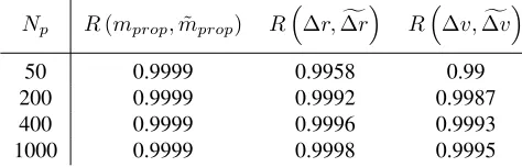
a Halton sequence. DACE is used with a regression model with polynomial of order 2 and an exponential correlation model. 200 test points are used to validate the surrogate models. Table 4 shows the correlation coefficientsR(mprop,m˜prop),R

∆r,∆fr

andR∆v,∆fv

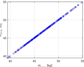
, for the 200 test points, considering models generated with different numbers Np of training points. Data in Table 4 show that 1000 training points generate an accurate surrogate model. Figures 8 show the relationship betweenmprop andm˜prop,∆rand

Table 4: Correlation coefficients between real functions and surrogate models for different number of training points.

Np R(mprop,m˜prop) R

∆r,∆fr

R∆v,∆fv

50 0.9999 0.9958 0.99

200 0.9999 0.9992 0.9987

400 0.9999 0.9996 0.9993

1000 0.9999 0.9998 0.9995

f

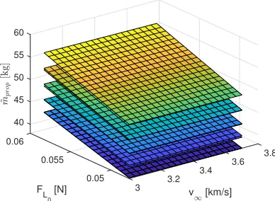
∆r,∆vand∆fvfor the 200 test points. As an example, the surfaces of the surrogate models form˜prop,∆fr and∆fv, for a given uncertain vectorξ, are shown in Figure 9, for different values ofv∞andFL0, on thex

andyaxis, and for fixed values of the other uncertain parameters.

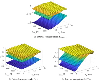
External Surrogate Models The external surrogate models are created using 150 training points generated

by Halton sequence, using DACE with polynomial of order 2 and gaussian correlation model. Figure 10 shows the external surrogate models ofSat the end of the iteration process described in Figure 4, for different

values ofv∞andIsp,L0(on thexandyaxis) and for fixed values of the other uncertain parameters.

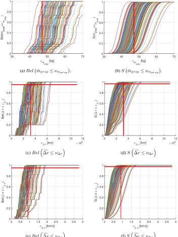
Results Figure 11 shows the curves ofBelandScorresponding to the 150 training points used to generate the external surrogate models. Each curve represented in Figure 11 corresponds, therefore, to a different vector of uncertain parameters, defined in the spaceΞ, and to its corresponding feasible and optimal control. The figures also represent, by means of red vertical lines, the considered values ofν¯mprop,ν¯∆randν¯∆v for

Problems (36) and (37). The red horizontal lines represent the chosen values of1−∆r,1−∆v,1−∆r,Sand 1−∆v,S. Feasible solutions to Problems (36) and (37) are given by the uncertain vectors and corresponding controls that, for the values ofν¯∆randν¯∆videntified by the red vertical lines, provide aBelorScurve that is above the red horizontal lines. Figures 12 show theBelcurves of the solutions of the iterative optimisation

process described in Figure 4 to solve Problem 36. The maximum number of allowed iterations is 40. In order to make the final results easier to visualise, Figures 13 show theBelcurves for the controls corresponding to

three uncertain vectors:

• the nominal uncertain vectorξnom(Table 2), represented in blue in Figure 13;

• the uncertain vector corresponding to the robust solution of Problem 36, identified byξrob, and repre-sented in black in Figure 13;

• an additional solution found during the iterative process described in Figure 4, which does not satisfy

40 45 50 55 m_prop [kg]

40 45 50 55

(a) Accuracy ofm˜prop.

0 0.5 1 1.5 2 2.5 3 3.5

r [km] 106

0 0.5 1 1.5 2 2.5 3 3.5 10

6

(b) Accuracy of∆fr.

0 0.2 0.4 0.6 0.8 1

v [km/s]

0 0.2 0.4 0.6 0.8 1

(c) Accuracy of∆fv.

Figure 8: Relationship betweenmpropandm˜prop(a),∆rand∆fr(b), and∆vand∆fv(c).

Figure 13.a shows that the nominal solution has a Belief of the objective, for the chosen value ofνmprop,

equal to 0.12. In order to get a Belief equal to 1 using the nominal control, the mass of propellant has to be increased to 55.5 kg. The Belief of the constraints for the nominal solution are both equal to 1, for the chosen values of ν∆r andν∆v. The robust solutionξrob, identified solving Problem 36, has a value of Bel(mprop ≤ ν¯mprop) higher than the one of the nominal solution, equal to 0.74. Moreover, when

considering the robust solution, the Belief of the propellant mass reaches 1 when the mass of propellant is equal to 49 kg. The improvement in the Belief of the objective comes with a small reduction in the values of

Bel(∆fr≤ν¯∆r)andBel(∆fv≤ν¯∆v), which are, however, still above the chosen values of 0.95. Finally, the solutionξnon−rob, represented in green, shows that the method presented in Figure 4 is capable of locating

many different solutions, characterised by different values of the Belief for the objective and the constraints. The Belief of the propellant mass corresponding toξnon−rob, which is equal to 1, is, in fact, higher than the corresponding Belief ofξrobandξnom. However, this comes with a reduction ofBel(∆fv≤ν¯∆v)to a value smaller than 0.95.

40

0.06 45

3.8 50

0.055 3.6

F

L 0

[N] 55

v [km/s] 60

3.4

0.05 3.2

3

(a) Internal surrogate modelm˜prop.

0 0.06 1

3.8 2

106

0.055 3.6

3

F

L 0

[N] _{v [km/s]}

4

3.4

0.05 3.2

3

(b) Internal surrogate model∆fr.

0 0.06

3.8 0.5

0.055 3.6

F

L 0

[N] _{v [km/s]}

1

3.4

0.05 3.2

3

(c) Internal surrogate model∆fv.

Figure 9: Example of internal surrogate modelsm˜prop(a),∆fr(b), and∆fv(c), for different values ofFL0

andv∞(xandyaxis), and for fixed values of the other uncertain parameters.

that, during the 40 iterations, the errors are:

|S˜ m˜prop≤ν¯mprop

−S m˜prop≤ν¯mprop

|<0.15

|S˜∆fr≤ν¯∆r

−S∆fr≤ν¯∆r

|<0.03

|S˜∆fv≤ν¯∆v

−S∆fv≤ν¯∆v

|<0.015

(38)

The errors are, therefore, limited to small values, and they are considered acceptable. It is important to stress that the aim of the proposed method is to obtain a surrogate model that is locally accurate in the region where the solutions of the considered problem are located; therefore, the surrogate models does not have to be globally accurate in the entire design space. Figure 14 shows the control solution, in terms of azimuth and elevation angles during the transfer, forξnomandξrob. The difference in the control shown in Figure 14 produces the difference in the Belief curves seen in Figure 13.

Computational Times In the following, the computational times required to complete each block in

Fig-ures 4 and 5 are given. The computational times refer to a code run on Matlab R2017b on a machine with Intel(R) Core(TM) i7-3770 CPU @3.40 GHz and 8 GB RAM. In particular, with reference to Figure 5:

(a) External surrogate model_S˜_m

prop.

(b) External surrogate model_S˜_{∆r. (c) External surrogate modelS}˜_∆v.

Figure 10: External surrogate modelS˜obj(a),S˜∆r(b), andS˜∆v(c).

• The creation of the internal surrogate models takes≈40sec;

• The computation of theBeltakes approximately3minutes, while the computation of the functionS

takes 8 seconds. The difference in these computational times is due to the fact that the computation of the Belief requires a maximisation over each one of the 48 focal elements, for each one of the three functionsm˜prop,∆frand∆fv. The computation of the functionSrequires, instead, only the evaluation of these functions at a given number of points.

With reference to Figure 4:

• The computation time required for the computation ofBelandS, for all theN training points inΞ,

is given by the multiplication ofN by the total computational time required to complete the diagram

flow in Figure 5 (4 minutes and 30 seconds, approximately). In this case, N = 150 and the total computational time to evaluate all the training points is, therefore, approximately11.25hours;

• The time required to create the external surrogate models forS, using the training points and DACE, is

≈0.5seconds;

30 40 50 60 70 m prop [kg] 0 0.2 0.4 0.6 0.8 1 Bel(m prop < mprop )

(a)Bel m˜prop≤νmprop

.

30 40 50 60 70

m prop [kg] 0 0.2 0.4 0.6 0.8 1 S(m prop < mprop )

(b)S m˜prop≤νmprop

.

0 2 4 6 8 10 12

r [km] 10

6 0 0.2 0.4 0.6 0.8 1 Bel( r < r )

(c)Bel∆fr≤ν∆r

0 2 4 6 8 10 12

r [km] 10

6 0 0.2 0.4 0.6 0.8 1 S( r < r )

(d)S∆fr≤ν∆r

0 0.5 1 1.5 2 2.5 3 3.5 4

v [km/s] 0 0.2 0.4 0.6 0.8 1 Bel( v < v ) (e)Bel f

∆v≤ν∆v

0 0.5 1 1.5 2 2.5 3 3.5 4

v [km/s] 0 0.2 0.4 0.6 0.8 1 S( v < v ) (f)S f

∆v≤ν∆v

Figure 11: Bel andS curves of the training points, corresponding to the objective (a and b), position

constraint (c and d), and velocity constraint (e and f).

process described in Figure 5 were to be realised, instead, at each function evaluation of the optimiser, the total computational time would have been10000×4.5min≈750hours;

• The computation time to computeBelandSforξoptis equal to the time required to complete the steps in Figure 5, that is, approximately 4 minutes and 30 seconds;

30 40 50 60 70

m prop

[kg] 0

0.2 0.4 0.6 0.8 1

Bel(m

prop

<

mprop

)

(a)Belm˜prop≤νmprop

.

0 2 4 6 8 10 12

r [km] 10

6 0

0.2 0.4 0.6 0.8 1

Bel(

r <

r

)

(b)Bel∆rf≤ν∆r

0 0.5 1 1.5 2 2.5 3 3.5 4

v [km/s]

0 0.2 0.4 0.6 0.8 1

Bel(

v <

v

)

(c)Bel∆vf≤ν∆v

Figure 12:BelandScurves of the results of the optimisation problem, corresponding to the objective (a),

position constraint (b), and velocity constraint (c).

CONCLUSION

This paper has presented the formulation and solution of the optimal control problem under uncertainty, where the uncertainty has been modelled using the Belief function of the Evidence Theory. In this work, the computation of the Belief function, which requires an optimisation over each focal element of the uncertainty space, has been sped up using internal surrogate models of the quantities to optimise. The original exact formulation of the problem, that uses the discontinuous Belief function, has then been transformed into an inexact formulation using a new continuous statistic function,S. The optimisation has then been realised on the surrogate of the functionS, rather than on the Belief. Moreover, by exploiting the correspondence between space of uncertainties and space of feasible and optimal controls, the optimisation has been realised on the space of uncertainties, rather than on the higher dimensional space of the controls. The method has been applied to the low-thrust transfer from Earth to asteroid Apophis. The considered uncertain parameters are the magnitude of the hyperbolic excess velocity at launch, and four parameters describing the thrust and specific impulse of the low-thrust engine and their variation during the transfer.

30 40 50 60 70

m prop

[kg]

0 0.2 0.4 0.6 0.8 1

Bel(m

prop

<

mprop

)

nom

rob

non-rob 55.5 kg

0.12 0.74

49 kg 1

(a)Belm˜prop≤νmprop

.

0 1 2 3 4 5 6 7 8

r [km] 10

6 0

0.2 0.4 0.6 0.8 1

Bel(

r <

r

)

nom

rob

non-rob

(b)Bel∆rf≤ν∆r

0 0.5 1 1.5 2

v [km/s] 0

0.2 0.4 0.6 0.8 1

Bel(

v <

v

)

nom

rob

non-rob

(c)Bel∆vf≤ν∆v

Figure 13: Belief of the nominal solution (ξnom), of the robust solution (ξrob), and of a non-robust solution (ξnon−rob).

control vector that provides a solution that is robust to uncertainties.

In this work, the proposed method has been applied to a problem with five uncertain parameters. The method could also be applied to higher dimensional problems. For higher dimensional problems, an increased computational time has to be expected. The increase in computational time is due to the increase in the number of focal elements over which to realise the maximisation for the computation of the Belief of the training points of the external surrogate models. In addition, an increased number of training points would likely be required to obtain sufficiently accurate initial external surrogate models.

Future work will be devoted to transform the constrained single-objective optimisation problem into a multi-objective optimisation problem, where the variablesνmprop,ν∆r,ν∆v,∆rand∆vare also minimised.

Moreover, the proposed method will be modified in order to extend the search for the robust solution to the space of all the admissible controls, so as to include also the non-feasible and non-optimal controls.

ACKNOWLEDGEMENTS

0 100 200 300 400 500 600 700 L [deg]

-100 -50 0

[deg]

rob

nom

0 100 200 300 400 500 600 700

L [deg] 0

5 10

[deg]

rob

nom

Figure 14: Controls (azimuth and elevation anglesαandβduring the transfer) corresponding toξnomand

ξrob.

REFERENCES

[1] M. Vasile, “Robust Mission Design Through Evidence Theory and Multiagent Collaborative Search,”

Annals of the New York Academy of Sciences, Vol. 1065, 2005, pp. 152–173.

[2] N. Croisard, M. Vasile, S. Kemble, and G. Radice, “Preliminary space mission design under uncer-tainty,”Acta Astronautica, Vol. 66, 2010, pp. 654–664.

[3] G. Shafer,A Mathematical Theory of Evidence. Princeton University Press, 1976.

[4] M. Vasile, E. Minisci, and Q. Wijnards, “Approximated Computation of Belief Functions for Robust De-sign Optimization,”53rd AIAA/ASME/ASCE/AHS/ASC Structures, Structural Dynamics and Materials Conference, Honolulu, Hawaii, 2012, 2012.

[5] A. P. Dempster, “Upper and Lower Probabilities Induced by a Multivalued Mapping,” The Annals of Mathematical Statistics, Vol. 38, No. 2, April 1967, pp. 325–339.

[6] L. Zhang, “Representation, independence, and combination of evidence in the Dempster-Shafer theory,”

Advances in the Dempster-Shafer theory of evidence(R. R. Yager, J. Kacpryk, and M. Fedrizzi, eds.),

ch. 3, pp. 51–69, New York: John Wiley and Sons, 1994.

[7] K. Sentz and S. Ferson, “Combination of Evidence in Dempster-Shafer Theory,” tech. rep., Sandia National Laboratories, 2002.

[8] M. Di Carlo, M. Vasile, and E. Minisci, “Multi-population inflationary differential evolution algorithm with adaptive local restart,”2015 IEEE Congress on Evolutionary Computation (CEC), 2015, pp. 632–

639.

[9] F. Zuiani, M. Vasile, A. Palmas, and G. Avanzini, “Direct transcription of low-thrust trajectories with finite trajectory elements,”Acta Astronautica, Vol. 72, 2012, pp. 108–120.

[10] M. Di Carlo, J. M. Romero Martin, and M. Vasile, “CAMELOT - Computational Analytical Multi-fidElity Low-thrust Optimisation Toolbox,”CEAS Space Journal, 2017.

[11] F. Zuiani and M. Vasile, “Extended analytical formulas for the perturbed Keplerian motion under a constant control acceleration,”Celestial Mechanics and Dynamical Astronomy, Vol. 121, No. 3, 2015,

pp. 275–300.