Schwarz preconditioning for high order edge element discretizations of the time-harmonic Maxwell's equations

Schwarz preconditioning for high order

edge element discretizations of the

time-harmonic Maxwell’s equations

M. Bonazzoli1_{, V. Dolean}1,2_{, R. Pasquetti}1_{, and F. Rapetti}1

AbstractWe focus on high order edge element approximations of waveguide

problems. For the associated linear systems, we analyze the impact of two Schwarz preconditioners, the Optimized Additive Schwarz (OAS) and the Optimized Restricted Additive Schwarz (ORAS), on the convergence of the iterative solver.

1 Introduction

High order discretizations of PDEs for wave propagation can provide a highly accurate solution with very low dispersion and dissipation errors. The result-ing linear systems can however be ill conditioned, so that preconditionresult-ing becomes mandatory. Moreover, the time-harmonic Maxwell’s equations with high frequency are known to be difficult to solve by classical iterative meth-ods, like the Helmholtz equation [3]. Domain decomposition methods are currently the most promising techniques for this class of problems (see [1, 2]). In order to simulate propagation in waveguide structures, we consider the second order time-harmonic Maxwell’s equation:

∇ ×

₁

µ∇ ×E

+ (iωσ−ω2ε)E=−iωJ, (1)

in the domainD ⊂_R3_{contained between two infinite parallel metallic plates}

y = 0 andy = Y. The wave propagates in thex-direction and all physical

1 _{Laboratoire J.A. Dieudonn´e, University of Nice Sophia Antipolis, Parc Valrose, 06108} Nice Cedex 02, France, e-mail:[email protected],victorita.dolean@unice. fr,[email protected],[email protected]

2 _{Department of Mathematics and Statistics, University of Strathclyde, Glasgow, UK,} e-mail:[email protected]

parameters (magnetic permeabilityµ, electrical conductivityσ, and electric permittivity ε) are invariant in the z-direction. Equation (1) assumes that the electric field E(x, t) = Re(E(x)eiωt_{) has harmonic dependence on time}

enforced by the imposed current sourceJ(x, t) = Re(J(x)eiωt_{),ω being the}

angular frequency. We work in a bounded sectionΩ = (0, X)×(0, Y) of D and solve the boundary value problem given by equation (1), where we set

J=0, with metallic boundary conditions on the waveguide walls:

E×n=0, onΓw={y= 0, y=Y},

and impedance boundary conditions at the waveguide entrance and exit:

(∇ ×E)×n+ iκn×(E×n) =gin, onΓin={x= 0},

(∇ ×E)×n+ iκn×(E×n) =gout, onΓout={x=X},

κ=ω√εµbeing the wavenumber andn= (nx, ny,0) the outward normal to

Γ =∂Ω. The assumptions onΩand on the physical parameters distribution are such thatE= (Ex, Ey,0), which yields∇ ×E= (0,0, ∂xEy−∂yEx).

The variational formulation of the problem is: findE∈V such that

Z

Ω

h

µϑE·v+ (∇ ×E)·(∇ ×v)i+

Z

Γin∪Γout

iκ(E×n)·(v×n)

=

Z

Γin

gin·v+

Z

Γout

gout·v, ∀v∈V,

withV ={v∈H(curl, Ω),v×n= 0 onΓw}, whereH(curl, Ω) is the space

of square integrable functions whose curl is also square integrable,ϑ= iωσ−

ω2_{ε, andµ is supposed constant. To write a finite element discretization of}

this problem we introduce a triangulation Th of Ω and a finite dimensional

subspaceVh⊂H(curl, Ω). The simplest possible conformal discretization for

the spaceH(curl, Ω) is given by the low orderN´ed´elec edge finite elements[6]: the local basis functions are associated with the oriented edges E={vi, vj}

of a given triangleT ofTh and they are given by

wE=λi∇λj−λj∇λi,

where theλ` are the barycentric coordinates of a point w.r.t. the nodev`.

2 High order edge finite elements

k= (k1, k2, k3) of weightk=k1+k2+k3(wherek1, k2, k3 are non negative

integers), we denote by λk _{the product λ}k1

1 λ k2

2 λ k3

3 . The basis functions of

polynomial degree r=k+ 1 over the triangleT are defined as

we=λkwE, (2)

for all edges E of the triangle T, and for all multi-indices k of weight k. Notice that these high order elements still yield a conformal discretization of

H(curl, Ω). Indeed, they are products between N´ed´elec elements, which are curl-conforming, and the continuous functionsλk_.

Fig. 1: The small triangles (shaded regions) and their small edges in the principal lattice of degreer= 3 (left) andr= 5 (right).

An interesting point of the proposed construction is the possible geomet-rical localization of the basis functions: the couples {k, E} appearing in (2) are in one-to-one correspondence with small edges e in the principal lattice of degreerofT (see Fig. 1). More precisely, the small edgee={k, E}is the small edge parallel toEthat belongs to the small triangle of barycentreGof coordinates λi(G) = 1/3+k_k+1i, i= 1,2,3. Thanks to the definition of the basis

the circulation of each basis function along a small edge is a constant that does not depend on the triangleT of the mesh.

Even if the described basis functions are very easy to generate, they don’t really form a basis as they arenot linearly independent. Indeed, for each small triangle which is not homothetic to the big one (the white ones in Fig. 1) one can check that the sum of the basis functions associated with its small edges is zero. Hence a redundant function should be eliminated for each ‘reversed’ small triangle.

3 Schwarz preconditioning

compare two domain decomposition preconditioners, theOptimized Additive Schwarz (OAS) and theOptimized Restricted Additive Schwarz (ORAS)

M_OAS−1 =

Nsub

X

s=1

RT_sA−_s1Rs, M_ORAS−1 = Nsub

X

s=1

e

RT_sA−_s1Rs,

where Nsub is the number of overlapping subdomains Ωs into which the

domain Ω is decomposed. The matrices As are the local matrices of the

subproblemswith impedance boundary conditions (∇×E)×n+ iκn×(E×n) as transmission conditions between subdomains.

In order to describe the matrices Rs,Res, let N be the set of degrees of

freedom andN =SNsub

s=1 Nsits decomposition into the subsets corresponding

to different subdomains. The matrix Rs is a #Ns×#N boolean matrix,

which is the restriction matrix fromΩ to the subdomainΩs. Its (i, j) entry

is equal to 1 if the i-th degree of freedom inΩs is thej-th one in the whole

Ω. Notice that RT

s is then the extension matrix from the subdomain Ωs to

Ω. The matrixResis a #Ns×#N restriction matrix, likeRs, but with some

of the unit entries associated with the overlap replaced by zeros: this would correspond to a decomposition into non overlapping subdomains Ωes ⊂ Ωs

(completely non overlapping, not even on their border!) (see [4]). This way

PNsub

s=1 ReT_sRs =I, that is the matrices Res give a discrete partition of unity

(which is made only of 1 and 0).

4 Numerical results

We present the results obtained for a waveguide with X = 0.0502 m,

Y = 0.00254 m, with the physical parameters: ε=ε0 = 8.85·10−12F m−1,

µ=µ0= 1.26·10−6H m−1 andσ= 0.15 S m−1. We consider three angular

frequenciesω1= 16 GHz,ω2= 32 GHz, andω3= 64 GHz, which correspond

to wavenumbers κ1 = 153.43 m−1, κ2= 106.86 m−1,κ3= 213.72 m−1,

vary-ing the mesh sizehaccording to the relationh2_·κ3_{= 2 [5].}

We solve the linear system with GMRES (with a tolerance of 10−6_),

start-ing with arandominitial guess, which ensures, unlike a zero initial guess, that all frequencies are present in the error. We compare the ORAS and OAS pre-conditioners, taking a stripwise subdomains decomposition, along the wave propagation, as shown in Fig. 2. Indeed, this is a preliminary testing of the discretization method and the preconditioner on a simple geometry which is the two-dimensional rectangular waveguide propagating only one mode; in this case, it is not necessary to consider more complicated or general decom-positions.

In our tests we vary the polynomial degreer=k+1, the angular frequency

ωand so the wavenumberκ, the number of subdomainsNsub, and finally the

1

Ω

2

Ω

Ω

Fig. 2: The stripwise decomposition of the domain.

Table 1: Influence ofk (ω=ω2,Nsub= 2, δovr= 2h).

k NdofsNiterNp Niter max|λ−1| #{λ:|λ−1|>1}#{λ:|λ−1|= 1}

0 282 179 5(10) 1.04e−1(1.38e+1) 0(4) 0(12) 1 884 559 6(15) 1.05e−1(1.63e+1) 0(8) 0(40) 2 1806 1138 6(17) 1.05e−1(1.96e+1) 0(12) 0(84) 3 3048 1946 6(21) 1.05e−1(8.36e+2) 0(16) 0(144) 4 4610 2950 6(26) 1.05e−1(1.57e+3) 0(20) 0(220)

Table 2: Influence of ω (k= 2,Nsub= 2,δovr= 2h).

κ NdofsNiterNp Niter max|λ−1| #{λ:|λ−1|>1}#{λ:|λ−1|= 1}

153.43 339 232 5(11) 2.46e−1(1.33e+1) 0(6) 0(45) 106.86 1806 1138 6(17) 1.05e−1(1.96e+1) 0(12) 0(84) 213.72 7335 4068 9(24) 3.03e−1(2.73e+1) 0(18) 0(123)

Table 3: Influence ofNsub (k= 2, ω=ω2, δovr= 2h).

Nsub Niter max|λ−1| #{λ:|λ−1|>1}#{λ:|λ−1|= 1}

2 6(17) 1.05e−1(1.96e+1) 0(12) 0(84) 4 10(27) 5.33e−1(1.96e+1) 0(38) 0(252) 8 19(49) 7.73e−1(1.96e+1) 0(87) 0(588)

Table 4: Influence ofδovr (k= 2,ω=ω2,Nsub= 2).

δovr Niter max|λ−1| #{λ:|λ−1|>1}#{λ:|λ−1|= 1}

of 1,2,4 mesh triangles along the horizontal direction. Tables 1–4 show the total number of degrees of freedom Ndofs, the number of iterations Niter for

convergence of GMRES preconditioned with ORAS(OAS) (NiterNp refers to

GMRES without any preconditioner), the greatest distance in the complex plane between (1,0) and the eigenvalues of the preconditioned matrix, the number of eigenvalues that have distance greater than 1, and the number of eigenvalues that have distance equal to 1 (up to a tolerance of 10−10_{). Indeed,}

ifAis the system matrix andM is the domain decomposition preconditioner, thenI−M−1_{Ais the iteration matrix of the domain decomposition method}

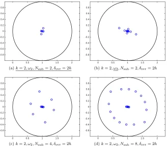
used as an iterative solver. So, here we see if the eigenvalues of the precon-ditioned matrix M−1A are contained in the unitary disk centered at (1,0). Notice that the matrix of the system doesn’t change whenNsub orδovrvary,

so in Tables 3–4 we don’t report Ndofs= 1806 and NiterNp= 1138 again. In

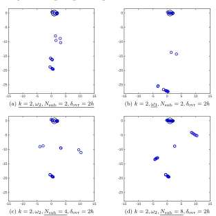
Figs. 3 and 4 we show for certain values of the parameters the whole spec-trum of the matrix preconditioned with ORAS and OAS respectively (notice that many eigenvalues are multiple).

0 0.5 1 1.5 2

-0.8 -0.6 -0.4 -0.2 0 0.2 0.4 0.6 0.8

(a)k= 2, ω2, Nsub= 2, δovr= 2h

0 0.5 1 1.5 2

-0.8 -0.6 -0.4 -0.2 0 0.2 0.4 0.6 0.8

(b)k= 2, ω3, Nsub= 2, δovr= 2h

0 0.5 1 1.5 2

-0.8 -0.6 -0.4 -0.2 0 0.2 0.4 0.6 0.8

(c)k= 2, ω2, Nsub= 4, δovr= 2h

0 0.5 1 1.5 2

-0.8 -0.6 -0.4 -0.2 0 0.2 0.4 0.6 0.8

(d)k= 2, ω2, Nsub= 8, δovr= 2h

-15 -10 -5 0 5 10 15 -25

-20 -15 -10 -5 0

(a)k= 2, ω2, Nsub= 2, δovr= 2h

-15 -10 -5 0 5 10 15

-25 -20 -15 -10 -5 0

(b)k= 2, ω3, Nsub= 2, δovr= 2h

-15 -10 -5 0 5 10 15

-25 -20 -15 -10 -5 0

(c)k= 2, ω2, Nsub= 4, δovr= 2h

-15 -10 -5 0 5 10 15

-25 -20 -15 -10 -5 0

(d)k= 2, ω2, Nsub= 8, δovr= 2h

Fig. 4: Spectrum in the complex plane of the OAS-preconditioned matrix.

We can see that the non preconditioned GMRES is very slow, and the ORAS preconditioning gives much faster convergence than the OAS precon-ditioning. Moreover, convergence becomes slower whenk,ωorNsubincrease,

or when the overlap size decreases; actually, when varyingk, the number of iterations for convergence using the ORAS preconditioner is equal to 5 for

k= 0 and then it stays equal to 6 fork >0.

Notice also that for 2 subdomains the spectrum is well clustered inside the unitary disk with the ORAS preconditioner, except for the case with

δovr=h, in which 3 eigenvalues are outside with distances from (1,0) equal

5 Conclusion

Numerical experiments have shown that Schwarz preconditioning improves significantly the GMRES convergence for different values of physical and numerical parameters, and that the ORAS preconditioner always performs much better than the OAS preconditioner. The only advantage of the OAS method is to preserve the symmetry of the preconditioner. Finally, it has been pointed out that the spectrum of the preconditioned matrix reflects the convergence qualities, which improve when the eigenvalues are well clustered inside the unitary disk centered at (1,0).

Acknowledgement This work was financed by the French National

Re-search Agency (ANR) in the framework of the project MEDIMAX, ANR-13-MONU-0012.

References

[1] V. Dolean, M. J. Gander, and L. Gerardo-Giorda. Optimized Schwarz methods for Maxwell’s equations. SIAM J. Sci. Comput., 31(3):2193– 2213, 2009.

[2] V. Dolean, M. J. Gander, S. Lanteri, J.-F. Lee, and Z. Peng. Effective transmission conditions for domain decomposition methods applied to the time-harmonic curl-curl Maxwell’s equations.J. Comput. Phys., 280:232– 247, 2015.

[3] O. G. Ernst and M. J. Gander. Why it is difficult to solve Helmholtz prob-lems with classical iterative methods. InNumerical analysis of multiscale problems, volume 83 of Lect. Notes Comput. Sci. Eng., pages 325–363. Springer, Heidelberg, 2012.

[4] M. J. Gander. Schwarz methods over the course of time. Electron. Trans. Numer. Anal., 31:228–255, 2008.

[5] F. Ihlenburg and I. Babuˇska. Finite element solution of the Helmholtz equation with high wave number. I. Theh-version of the FEM. Comput. Math. Appl., 30(9):9–37, 1995.

[6] J.-C. N´ed´elec. Mixed finite elements inR3.Numer. Math., 35(3):315–341, 1980.

[7] F. Rapetti. High order edge elements on simplicial meshes. M2AN Math. Model. Numer. Anal., 41(6):1001–1020, 2007.