City, University of London Institutional Repository
Citation
:
Wang, Q. & Grattan, K. T. V. (2017). Suppression of subsidiary fringes in white
light interferometry utilising two-wavelength light source. Optics Communications, 403, pp.
121-126. doi: 10.1016/j.optcom.2017.07.029
This is the accepted version of the paper.
This version of the publication may differ from the final published
version.
Permanent repository link:
http://openaccess.city.ac.uk/17909/
Link to published version
:
http://dx.doi.org/10.1016/j.optcom.2017.07.029
Copyright and reuse:
City Research Online aims to make research
outputs of City, University of London available to a wider audience.
Copyright and Moral Rights remain with the author(s) and/or copyright
holders. URLs from City Research Online may be freely distributed and
linked to.
Suppression of subsidiary fringes in white light interferometry
utilising two-wavelength light source
Qi Wang 1 and Kenneth Thomas V. Grattan 2
1 Department of Physics, Huazhong University of Sci. & Tech., Wuhan, 430074, P. R. China 1 Contact address: 15 Cascades Road, Pakuranga, Auckland, New Zealand
2
Photonics & Instrumentation Research Centre, City, University of London, Northampton Square, London, EC1V 0HB, UK
*Corresponding author: qi_wang_58@hotmail.com
This paper underpins the use of white-light interferometers for a range of measurement applications and analyses and compares two methods for suppressing the subsidiary fringes in white-light correlograms using a two-wavelength light source. One of the methods adds the intensities of the two two-wavelength components and the other multiplies them and the peak intensity difference between the central fringe and the subsidiary fringes is investigated. A mathematical expression for a rapid estimation of the optimum wavelength difference between the two wavelengths is given for suppressing the subsidiary fringes. The effects of the intensities of the two wavelength components have also been investigated.
Key words
: Interferometry, metrology.1.
Introduction
White-light interferometric (WLI) sensors have been investigated by many researchers over a number of years for a wide range of applications, which include thickness gauges [1], optical fiber displacement sensors [2], surface profilers and topography and surface shape measurement [3 - 8], object shape [9] and microscopy [10]. They remain an important and topical area of advanced sensor research [11]. One of the advantages of such WLI sensors is that they can avoid the phase ambiguity by distinguishing the central fringe of the correlograms. Light-emitting diodes (LEDs) are energy efficient, light in weight, and low in cost when compared to conventional light sources and thus are well suited to use in white-light interferometry, especially for ‘in-the-field’ applications. However, a key issue is that the central fringe of a correlogram illuminated by a LED may not be easily distinguished by comparing the peak intensities of the interference fringes, especially when noise is present. Larkin has developed the efficient algorithms for the detection of the envelope of white-light correlograms [12], which may help to distinguish the central fringe. Two-wavelength methods can also be used to enhance the central fringe of the low coherence correlograms [13 - 17]. With a two-wavelength light source, a beat fringe pattern is generated in the correlogram and hence the subsidiary fringes are suppressed.
There are two familiar types of two-wavelength methods. One of them is to add the intensities of the two wavelength components [13 - 15, 17], and the other is to multiply them [16]. The fringe patterns produced by adding may be termed ‘added correlograms’ and those produced by multiplying as ‘multiplied correlograms’.
As shown in the upper part of Fig. 1, depending on the two wavelengths used, the second largest fringe in an added correlogram or a multiplied correlogram can either be the first subsidiary fringe or the largest fringe in the first
subsidiary fringe packet. In order to suppress the subsidiary fringes, the normalized peak intensity difference between the central fringe and the first subsidiary fringe (NPID1), and the normalized peak intensity difference between the central fringe and the largest fringe in the first subsidiary fringe packet (NPID2) will be examined. A mathematical expression will then be given for a rapid estimation of the optimum wavelength difference for suppressing the subsidiary fringes when the coherence length and the shorter wavelength are given. The effects of the intensities of the wavelength components on the NPID1 and NPID2 of the correlograms will also be examined.
)} 2 cos( ] ) ( exp[ 1 { ) ( 2 x l x a x
I , (1)
where a represents the amplitude of the central fringe of the
correlogram, λ represents the central wavelength of the light
source, x represents the optical path difference (OPD) of the
interferometer, and l represents the coherence length of the
light source.
When two low coherence sources of different colors are used to illuminate the Michelson interferometer, the correlograms of the two wavelength components can be expressed respectively as
)} 2 cos( ] ) ( exp[ 1 { ) ( 1 2 01 1 x l x I x
I (2a)
and )} 2 cos( ] ) ( exp[ 1 { ) ( 2 2 02 2 x l x I x
I , (2b)
where 1 and 2 represent the central wavelengths, I01
and I02 represent the average intensities of the wavelength
components.
By multiplying Eq. (2a) and Eq. (2b), the multiplied correlogram can be written as
, ) ( ) ( )} 2 cos( ) 2 cos( ] ) ( 2 exp[ 1 { )} 2 cos( ] ) ( exp[ ) 2 cos( ] ) ( exp[ 2 { ) ( ) ( ) ( 2 1 2 0 2 2 1 2 0 2 1 x I x I x x l x I x l x x l x I x I x I x I d a m (3)
where I0 I01I02,
)} 2 cos( ] ) ( exp[ ) 2 cos( ] ) ( exp[ 2 { ) ( 2 2 1 2 0 x l x x l x I x Ia
represents the added correlogram, and
)} 2 cos( ) 2 cos( ] ) ( 2 exp[ 1 { ) ( 2 1 2 0
x x
l x I
x
Id
represents the arithmetic difference between the added correlogram and the multiplied correlogram.
The added correlogram can be rewritten as )} 2 cos( ) cos( ] ) ( exp[ 1 { ) ( 2 a m a x x l x A x I
(4a)
and the arithmetic difference Id(x) can be rewritten as
)]} 2 / 2 cos( ) 2 ][cos( ) ( 2 exp[ 2 { 4 ) ( 2 a m d x x l x A x I , (4b)
where A2I01I02is the amplitude of the central fringe of
the added correlogram, a 212/(12) is the
average wavelength, and m 12/12 is the
modulation wavelength. When the two wavelengths used are
0.78µm and 0.67 µm, the average wavelength is approximately 0.72µm and the modulation wavelength is approximately 4.75 µm.
It should be noted that Eq. (4a) represents the added correlograms when the intensities of the wavelength components are equal.
Eq. (4b) shows that the arithmetic difference consists of two oscillating terms. One of these oscillates at the
modulation wavelength (m) and the other oscillates at a
half of the average wavelength (a/2).
3.
Comparision between the added correlogram
and the multiplied correlogram
Fig. 1 plots the added correlogram (given by Eq.(4a)), the multiplied correlogram (given by Eq.(3)), and the arithmetic
difference between them, when the amplitude
A
is unity.In the upper part of Fig. 1, the envelopes of the correlograms are modulated by the beat effect generated by the two wavelength components. The beat effect suppresses the subsidiary fringes.
In the upper part of Fig. 1, we also find the subsidiary fringes in the multiplied correlogram are smaller than those in the added correlogram.
There are two sinusoidal oscillations that can be seen in the graph in the lower part of Fig. 1. The faster oscillation has a wavelength of about 0.36 µm, which is a half of the average wavelength. The slower oscillation has a wavelength of about 4.7 µm, which is the same as the modulation wavelength. This is consistent with the theoretical result given by Eq. (4b) where the two oscillating terms are present.
From Fig. 1, it can also be seen that the central fringe of the arithmetic difference is about a quarter of the size of the central fringe in the added correlogram. This is consistent with the theoretical results given by Eq. (4a) and Eq. (4b), where the number 4 can be seen in the denominator in Eq.(4b).
By examining the graph in the lower part of Fig. 1, the arithmetic difference has been maximized at the quadrature positions of the correlograms, and minimized when the correlograms reach the extreme values.
-6 -4 -2 0 2 4 6
0 1 2 In te n si ty
-6 -4 -2 0 2 4 6
0 0.5 1
OPD of the interferometer (µm)
[image:3.612.322.541.538.707.2]Fig. 1. The added correlogram Ia (upper graph in upper part), the multiplied correlogram Im (lower graph in upper part), and the difference Id (graph in lower part). Coherence length: 7.0 µm; two wavelengths: 0.78µm and 0.67 µm.
4.
Estimation of NPID1
From Eqs. (3), (4a) and (4b), the peak intensity of the first subsidiary fringe of added correlogram can be given by
)] cos( ] ) ( exp[ 1 [ ) ( 2 m a a a a l A I
, (5a)
and the peak intensity of the first subsidiary fringe of multiplied correlogram can be estimated by
. )} ( cos ] ) ( 2 exp[ 1 { 2 )} cos( ] ) ( exp[ 1 { ) ( 2 2 2 m a a m a a a m l A l A I (5b) If the effect of the coherence envelope is neglected, the NPID1 of added correlogram can be estimated by
) cos( 1 ) ( 2 1 NPID m a a a a A I A
(6a)
and that of multiplied correlogram can be estimated by
. ) ( sin 2 1 ) cos( 1 ) ( 2 1 NPID 2 m a m a a m m A I A (6b)
By comparing Eq.(6a) with Eq. (6b), it is clear that, for a given pair of wavelengths, the NPID1 of the multiplied correlogram is greater than that of the added correlogram.
It should be noted that Eq. (6a) can be used for estimating the NPID1 of added correlogram when the average intensities of the wavelength components are equal.
5.
Estimation of NPID2
In a two-wavelength correlogram, the second largest fringe may not be the first subsidiary fringe. From Fig. 1, it can be seen that the second largest fringe in a two-wavelength correlogram can either be the first subsidiary fringe or the largest fringe in the first subsidiary fringe packet. Which fringe is the second largest in a two-wavelength correlogram depends on the two wavelengths that are used for illumination.
From Eq. (4a), the NPID2 of added correlogram can be estimated by ]] ) ( exp[ 1 [ 2 2 NPID 2 l m a
. (7a)
Similarly, from Eqs. (3), (4a) and (4b), NPID2 of multiplied correlogram can be estimated by
. ]]} ) ( 2 exp[ 1 [ 2 1 ] ) ( exp[ 1 { 2 2 NPID 2 2 l l m m m (7b) Eq. (7a) can be written as
] ) ( exp[ 1 2 NPID 2 l m a
(8a)
and Eq. (7b) can be written as
. ]} ) ( exp[ 1 ]}{ ) ( exp[ 3 { 2 1 2 NPID 2 2 l l m m m (8b)
The details needed to derive Eq. (8b) can be found in the Appendix. By comparing Eq.(8a) with Eq. (8b), it is clear that, for a given pair of wavelengths, the NPID2 of the multiplied correlogram is greater than that of the added correlogram.
It should be noted that Eq. (8a) can be used for estimating the NPID2 of added correlogram when the average intensities of the wavelength components are equal.
6.
Optimum wavelength difference
In order to estimate the optimum wavelength difference, it is useful to further simplify Eqs. (6) and Eqs. (8).
When m a, Eq. (6a) and Eq. (6b) can be written
respectively as 2 2 1 2 1 2 ) ( 2 1 NPID
a (9a)
and 2 2 1 2 1 2 ) ( 4 1 NPID
m . (9b)
In order to proceed with the analysis, Eqs (8) can be expanded into a power series and only the first term is kept. Then Eq.(8a) can be approximated by
2 2 1 2 1 ) ) ( ( 2 NPID l
a , (10a)
and Eq. (8b) can be approximated by 2 2 1 2 1 ) ) ( ( 2 2 NPID l
m . (10b)
Eqs. (9) indicate that, for a given pair of wavelengths, the NPID1 of the multiplied correlogram is about two times the NPID1 of the added correlogram. Further, Eqs. (10) indicate that, for a given pair of wavelengths, the NPID2 of the multiplied correlogram is about two times the NPID2 of the added correlogram.
Eqs. (9) and Eqs. (10) show the effects of the wavelength difference on NPID1 and NPID2 of the two-wavelength correlograms. Eqs. (9) show that NPID1 increases as the wavelength difference increases, whereas Eqs. (10) indicate that NPID2 decreases as the wavelength difference increases. This suggests that there should be an optimum wavelength difference at which NPID1 be equal to NPID2 and therefore the peak-intensity difference between the central fringe and the second largest fringe be maximized.
For the added correlogram, the optimum wavelength difference can be obtained by letting Eq. (9a) be equal to Eq.(10a). For the multiplied correlogram, the optimum wavelength difference can be obtained by letting Eq.(9b) be equal to Eq.(10b). These lead to the same equation that can be written as
) (
where OP210 is the optimum wavelength difference.
Eq. (11a) can be used to determine the optimum
wavelength difference OP for both added correlogram and
that of multiplied correlogram.
Since 21OP, Eq. (11a) can be written as
2 1 2
1 3
1 2
3 2 2
l OP OP OP
. (11b)
Since 1OP0, we have
2 1 2
1 3 2
OP OP
, (12)
and therefore the third term in right hand side of Eq. (11b) is negligible. Then the following can be stated
1 3
1 2
3 2 2
l OP OP
. (13)
The right hand side of Eq. (13) can be approximated by a constant. Therefore, the optimum wavelength difference can be calculated by
l OP 1 0.6 1
, (14)
where 1 is the shorter wavelength and l the coherence
length. The number 0.6 used in the above was determined by trial and error. The criterion to determine the number is whether the NPID1 is close to the NPID2 in the generated
correlogram with the calculated OP.
Eq. (14) can be used for the rapid estimation of the optimum wavelength difference for suppressing the subsidiary fringes.
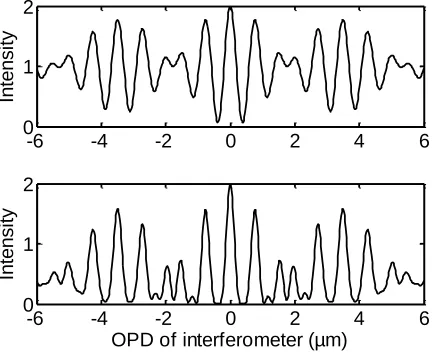
Figs. 2 show examples of the correlograms with the optimum wavelength difference given by Eq. (14). It can be seen from the figures that the peak intensity of the first subsidiary fringe is about the same as that of the largest fringe in the first subsidiary fringe packet, and therefore
NPID1NPID2. The figures also show that, with the
wavelength difference given by Eq. (14), the subsidiary fringes in the correlograms are satisfactorily suppressed.
-6 -4 -2 0 2 4 6
0 1 2
In
te
n
si
ty
-6 -4 -2 0 2 4 6
0 1 2
In
te
n
si
ty
OPD of interferometer (µm) (a)
-6 -4 -2 0 2 4 6
0 1 2
In
te
n
si
ty
-6 -4 -2 0 2 4 6
0 1 2
In
te
n
si
ty
OPD of interferometer (µm) (b)
-100 -5 0 5 10
1 2
In
te
n
si
ty
-100 -5 0 5 10
1 2
In
te
n
si
ty
OPD of interferometer (µm) (c)
Fig. 2. Added correlogram (upper graph) and multiplied correlogram (lower graph) (a) when l = 7.0 µm,
1
= 0.70 µm andOP
= 0.17µm (b) when l = 10 µm,
1
= 0.50 µm andOP
=0.087µm (c) when l = 15 µm,
1
= 1.5 µm andOP
=0.37µm.
[image:5.612.326.543.59.441.2] [image:5.612.49.261.551.729.2]0.5 0.7 0.9 1.1 1.3 1.5 -0.2 -0.1 0 0.1 0.2 0.3 P D 2 1
Shorter wavelength (µm)
PD21 when coherence length is 5 µm PD21 when coherence length is 10 µm PD21 when coherence length is 15 µm
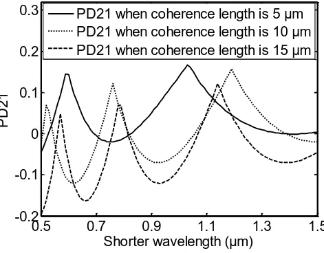
Fig. 3. PD21 of correlograms versus the shorter wavelength when the coherence length is 5 µm, 10 µm, and 15 µm. The correlograms are generated with the optimum wavelength difference given by Eq. (14).
In order to examine the usefulness of Eq. (14), the percentage difference between NPID2 and NPID1 is defined as 1 NPID 1 NPID 2 NPID
PD21 . (15)
For the optimum suppressing of the subsidiary fringes, the smaller the absolute value of PD21, the better. When PD21 is equal to zero, the peak-intensity difference between the central fringe and the second largest fringe is maximized. Fig. 3 shows PD21s of simulated correlograms with the optimum wavelength difference given by Eq. (14). The simulation results show that the absolute values of PD21s of the correlograms are less than 20% when the shorter wavelength varies from 0.50 µm to 1.50 µm and the coherence length varies from 5.0 µm to 15 µm. In the computer simulation carried out, PD21s are calculated by determining the peak intensity of the first subsidiary fringe and that of the first subsidiary fringe packet.
It should be noted that graphs in Fig. 3 are from added correlograms. Almost exactly the same graphs have been plotted with multiplied correlograms, (which for brevity are not included in the paper). The simulation results show that Eq.(14) can be used for estimating the optimum wavelength
difference for both added and multiplied correlograms.
7.
Effects of the intensities of the two wavelength
components
Previous researchers appear to have overlooked the effects of the intensities of the two wavelength components [9 - 13]. In practical WLI sensors, it is clear that the intensities of the two wavelength components may vary in use for measurement applications. Hence, it is necessary to investigate the effects of the intensities on NPID1 and NPID2 of the two-wavelength correlograms.
The intensity ratio RI02/I01 is defined as the
average intensity of the longer wavelength over that of the shorter wavelength.
From Eq. (2a) and Eq. (2b), the normalized added correlograms can be expressed as
.
)]}
2
cos(
]
)
(
exp[
1
[
)]
2
cos(
]
)
(
exp[
1
){[
)
1
(
1
(
)
(
2 2 1 2
x
l
x
R
x
l
x
R
x
I
a
(16a) Also from Eq. (2a) and Eq. (2b), the normalized multiplied correlograms can be expressed as.
)]
2
cos(
]
)
(
exp[
1
[
)]
2
cos(
]
)
(
exp[
1
[
2
1
)
(
2 2 1 2
x
l
x
x
l
x
x
I
m
(16b) From Eq. (16b), it is clear that the normalized multiplied correlograms are independent of the intensity ratio. Therefore, NPID1 and NPID2 of the multiplied correlogram are independent of the intensity ratio.Graphs given as Fig. 4 shows the normalized added
correlograms given by Eq. (16a) when the intensity ratio R is
0.1, 0.3, and 0.8 respectively. It can be seen from the graphs that the beat effect varies with the intensity ratio.
-100 -5 0 5 10
1 2 In te n si ty R = 0 .1
-100 -5 0 5 10
1 2 In te n si ty R = 0 .3
-100 -5 0 5 10
1 2 In te n si ty R = 0 .8
OPD of interferometer (µm)
Fig. 4. The added correlograms given by Eq. (16a) when the intensity ratio is 0.1, 0.3, and 0.8 respectively. Coherence length: 7.0 µm; two wavelengths: 0.78 µm and 0.67 µm.
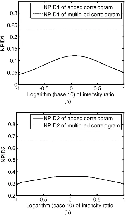
NPID1 of the simulated added correlogram and the multiplied correlogram is determined when the intensity ratio varies. The simulation results are displayed in Fig. 5(a) when the logarithm of the intensity ratio varies from –1 to 1 and so the intensity ratio varies from 0.1 to 10.
Fig. 5(a) shows the NPID1 of the multiplied correlograms is independent of the intensity ratio, whereas the NPID1 of the added correlograms is maximized when the intensity ratio is about unity.
[image:6.612.45.272.54.228.2] [image:6.612.319.543.339.516.2]are 0.67 µm and 0.78 µm, these being important wavelengths available from common, inexpensive LEDs.
-1 -0.5 0 0.5 1
0 0.05 0.1 0.15 0.2 0.25 0.3
Logarithm (base 10) of intensity ratio
N
P
ID
1
NPID1 of added correlogram NPID1 of multiplied correlogram
(a)
-1 -0.5 0 0.5 1
0.2 0.3 0.4 0.5 0.6 0.7 0.8
Logarithm (base 10) of intensity ratio
N
P
ID
2
NPID2 of added correlogram NPID2 of multiplied correlogram
(b)
Fig. 5. (a) NPID1 varying with the logarithm of the intensity ratio (b) NPID2 varying with the logarithm of the intensity ratio. Coherence length: 7.0µm; two wavelengths: 0.78 µm and 0.67 µm.
The lower graph in Fig. 5(a) also indicates that the NPID1 of the added correlograms peaks when the intensity ratio is slightly greater than unity. In other words, the NPID1 of the added correlograms is maximized when the intensity of the longer wavelength is slightly greater than that of the shorter wavelength. This can be explained by the fact that the average wavelength of added correlogram increases as the intensity ratio increases and the amplitude of the first subsidiary fringes decreases as the average wavelength increases.
NPID2 of the simulated added correlogram and the multiplied correlogram is determined when the intensity ratio varies. The simulation results are displayed in Fig. 5(b) when the logarithm of the intensity ratio varies from –1 to 1 and so the intensity ratio varies from 0.1 to 10.
Fig. 5(b) shows the NPID2 of the multiplied correlograms is independent of the intensity ratio, whereas the NPID2 of the added correlograms is maximized when the intensity ratio is about one.
Fig. 5(b) shows that the NPID2 of the multiplied correlograms is about twice the maximum NPID2 of the added correlograms. This is consistent with the results given by Eq. (8a) and Eq. (8b). Eq.(8a) gives a NPID2 of 0.37 for the added correlograms and Eq.(8b) gives a NPID2 of 0.67 for the multiplied correlograms when the coherence length is 7 µm and the two wavelengths are 0.67 µm and 0.78 µm.
8.
Conclusions and relevance to creating better
optical fiber sensors
Two methods for suppressing subsidiary fringes in white-light interferometry with two-wavelength white-light source have been analyzed and compared. Mathematical expressions have been given for estimating NPID1 and NPID2 of added and multiplied correlograms.
A mathematical expression (Eq. (14)) has also been given for a rapid estimation of the optimum wavelength difference between the two wavelengths for suppressing the subsidiary fringes in added and multiplied correlograms. For the correlograms with the wavelength difference given by Eq.(14), the PD21s have been shown to be less than 20 percent when the shorter wavelength varies from 0.50 µm to 1.5 µm and the coherence length varies from 5.0 µm to 15µm.
The normalized multiplied correlograms are independent of the intensities of the wavelength components, whereas the beat effect in the added correlograms is maximized when the intensities of the wavelength components are about equal.
For a given pair of wavelengths, the NPID1 of the multiplied correlogram is about two times the maximum NPID1 of the added correlogram and the NPID2 of the multiplied correlogram is about two times the maximum NPID2 of the added correlogram.
[image:7.612.39.263.85.462.2]Appendix
Eq. (7b) can be written as
. ]} ) ( exp[ 1 ]}{ ) ( exp[ 1 { 2 1 ] ) ( exp[ 1
2 NPID
2 2
2
l l
l
m m
m m
(A1) Then, the NPID2 of multiplied correlogram can be expressed as
. ]} ) ( exp[ 1 ]}{ ) ( exp[ 3 { 2 1
2 NPID
2 2
l l
m m
m
(A2)
References
1. P. A. Flournoy, R. W. McClure, and G. Wyntjes,
“White-light interferometric thickness gauge,” Appl.
Opt. 11, 1907-1915 (1972).
2. A. Koch and R. Ulrich, “Fibre-optic displacement
sensor with 0.02m resolution by white-light
interferometry,” Sensors and Actuators A, 25-27,
201-207 (1991).
3. P. J. Caber, “Interferometric profiler for rough surfaces”
Appl. Opt., 32, 3438-3441 (1993).
4. S. Tereschenko, P. Lehmann, L. Zellmer and A.
Brueckner-Foit “Passive vibration compensation in scanning white-light interferometry”, Appl Opt. 10;55(23), 6172-82 (2016) doi: 10.1364/AO.55.006172.
5. P. Sandoz and G. Tribillon, “Profilometry by zero-order
interference fringe identification”, J. Modern Opt., 40,
1691-1700 (1993).
6. L. Deck and P. de Groot, “High-speed noncontact
profiler based on scanning white-light interferometry”,
Appl. Opt., 33, 7334-7338 (1994).
7. Z. Lei, X. Liu, L. Chen, W. Lu and S. Chang, “A novel
surface recovery algorithm in white light
interferometry”, Measurement, 80, 1–11, (2016)
8. A. Harasaki, J. Schmit, and J. C. Wyant, “Improved
vertical-scanning interferometry”, Appl. Opt., 39,
2107-2115 (2000).
9. P. Pavliček and E. Mikeska, “Fast white-light
interferometry with Hilbert transform evaluation”, Proc. SPIE 10142, 20th Slovak-Czech-Polish Optical Conference on Wave and Quantum Aspects of
Contemporary Optics, 101420Y (2016),
doi:10.1117/12.2261951
10. G. S. Kino and S. S. C. Chim, “Mirau correlation
microscope”, Appl. Opt., 29, 3775-3783 (1990).
11. Photonics Media “White Light Interferometry”
https://www.photonics.com/Splash.aspx?Tag=white-light+interferometry (2017)
12. K. G. Larkin, “Efficient nonlinear algorithm for
envelope detection in white light interferometry”, J.
Opt. Soc. Am. A, 13, 832-843 (1996).
13. S. Chen, K. T. V. Grattan, B. T. Meggitt, and A. W.
Palmer, "Instantaneous fringe-order identification using
dual broadband sources with widely spaced
wavelengths", Electron. Lett., 29, 334-335 (1993).
14. Y. J. Rao, Y. N. Ning and D. A. Jackson, "Synthesized
source for white-light sensing systems", Opt. Lett., 18,
462-464 (1993).
15. D. N. Wang, Y. N. Ning, K. T. V. Grattan, A. W.
Palmer, and K. Weir, “Characteristics of synthesized light sources for white-light interferometric systems”,
Opt. Lett., 18, 1884-1886 (1993).
16. Y. J. Rao, D. A. Jackson, "Improved synthesized source
for white light interferometry", Electron. Lett., 30,
1440-1441 (1994).
17. D. N. Wang, Y. N. Ning, K. T. V. Grattan, A. W.
Palmer, and K. Weir "The optimized wavelength combinations of two broadband sources for white light
interferometry", IEEE/OSA J. Lightwave Technol. 12,
909-916 (1994).
18. K. T. V. Grattan and B. T. Meggitt “Optical Fibre