City, University of London Institutional Repository
Citation
:
Klein, N., Kneib, T., Marra, G., Radice, R., Rokicki, S. R. and McGovern, M. (2019). Mixed Binary-Continuous Copula Regression Models with Application to Adverse Birth Outcomes. Statistics in Medicine, 38(3), pp. 413-436. doi: 10.1002/sim.7985This is the accepted version of the paper.
This version of the publication may differ from the final published
version.
Permanent repository link: http://openaccess.city.ac.uk/id/eprint/20470/
Link to published version
:
http://dx.doi.org/10.1002/sim.7985Copyright and reuse:
City Research Online aims to make research
outputs of City, University of London available to a wider audience.
Copyright and Moral Rights remain with the author(s) and/or copyright
holders. URLs from City Research Online may be freely distributed and
linked to.
Mixed Binary-Continuous Copula Regression
Models with Application to Adverse Birth
Outcomes
Nadja Klein, Thomas Kneib
Chair of Statistics
Georg-August-University G¨ottingen
Giampiero Marra
Department of Statistical Science University College London
Rosalba Radice
Department of Economics, Mathematics and Statistics Birkbeck, University of London
Slawa Rokicki
Department of Economics, Mathematics and Statistics Birkbeck, University of London
Mark E. McGovern
Geary Institute University College Dublin
Abstract
Bivariate copula regression allows for the flexible combination of two arbitrary, continuous marginal distributions with regression effects being placed on potentially all parameters of the resulting bivariate joint response distribution. Motivated by a study examining the risk factors of adverse birth outcomes, we consider mixed binary-continuous responses that extend this framework to the situation where one response variable is discrete (more precisely binary) while the other response remains continuous. Utilizing the latent continuous representation of binary regression models, we implement a penalized likelihood based approach for the resulting class of copula regression models and employ it in the context of modelling jointly gestational age and the presence/absence of low birth weight. The analysis strongly benefits from the flexible specification of regression effects including nonlinear effects of continuous covariates and spatial effects.
Key words: Adverse birth outcomes; Copula; Latent variable; Mixed discrete-continuous distributions; Penalised maximum likelihood; Penalised splines.
1
Introduction
and mental disability and chronic health problems are high (Slattery and Morrison, 2002). Moreover, LBW is associated with poor educational and labor force outcomes in adolescence and adulthood including lower scores on academic achievement tests, lower rates of high school completion, lower income, and higher social assistance take-up (Almond and Currie, 2011; Behrman and Rosenzweig, 2004; Black et al., 2007; Hack et al., 2002; McGovern, 2013; Oreopoulos et al., 2008).
Although both LBW and gestational age are predictors of future health, modelling these outcomes jointly is essential for a number of reasons. First, birth weight and ges-tational age are highly correlated, confounded by factors such as intrauterine growth restriction (Slattery and Morrison, 2002). In addition, risk factors for LBW such as socio-economic status, smoking, and maternal age are also the same risk factors for preterm birth. Finally, evidence suggests that the impact of LBW on health may be elevated by low gestational age, and vice-versa (Hediger et al., 2002). Thus, mod-elling these outcomes independently would present a confounded picture of who is most vulnerable to poor infant health and how best to intervene. A more accurate picture is revealed by modelling these outcomes jointly.
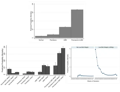
We use data from the North Carolina State Center for Health Statistics to show the probability of mortality by birth weight and prematurity. The data include all births in the state from 2007 to 2013 and provide information on maternal characteristics, delivery characteristics, and infant birth and death outcomes, at the county level for a total number of n= 109,380 observations. Figure 1 (top) shows the probability of infant mortality for premature infants (but not LBW), LBW infants (but not prema-ture), premature and LBW infants, and infants without these conditions (“normal”). The probability of death is more than two times higher for infants that are both LBW and premature, compared to those that are only LBW. In addition, the risk associated with LBW and prematurity varies depending on maternal characteristics. For instance, Figure 1 (bottom left) shows that probability of death for premature and LBW infants is significantly higher for infants born to black mothers than those born to white or other race mothers, whereas the rate of infant mortality is similar across mother’s race for infants that are LBW (but not premature).
To model adequately these data, we consider bivariate copula regression models in the same vein as Marra and Radice (2017a), Radice et al. (2016) and Klein and Kneib (2016). Generally, these works utilize copulas to construct flexible bivariate response distributions where both margins are either binary or continuous. Following an ap-proach similar to Marra and Radice (2017a), we implement a simultaneous penalized likelihood method which employes copulae to combine a binary response variable (low birth weight in our case) and a continuous outcome (gestational age) while account-ing for several types of non-Gaussian dependencies. To facilitate the methodological developments, for the binary part of the model, we use the latent response represen-tation of binary regression models. To go beyond simplistic mean regression settings, the marginal and copula parameters are related to regression predictors of structured additive form.
0
.01
.02
.03
.04
Predicted Probability (Mortality)
Normal Premature LBW Premature & LBW
0
.01
.02
.03
.04
Predicted Probability (Mortality)
Normal Birth, WhiteNormal Birth, BlackNormal Birth, OtherPremature, WhitePremature, BlackPremature, Other
LBW, WhiteLBW, BlackLBW, Other
Premature & LBW, WhitePremature & LBW, BlackPremature & LBW, Other
0
.1
.2
.3
24 25 26 27 28 29 30 31 32 33 34 35 36 37 38 39 40 41 42 24 25 26 27 28 29 30 31 32 33 34 35 36 37 38 39 40 41 42
Not Low Birth Weight Low Birth Weight (<2500g)
Predicted Probability (Mortality)
[image:4.595.89.507.66.389.2]Weeks of Gestation
Figure 1: Probability of infant mortality by infant birth category (top), by infant birth category and mother’s race (bottom left) and by weeks of gestation, stratified by low birth weight status (bottom right). Error bars show the 95% confidence interval. Source: North Carolina Vital Statistics (combined birth and death records), 2007-2013.
separately. As shown in simulation by Marra and Radice (2017a), estimating all the model’s parameters simultaneously offers computational and efficiency gains, hence the simultaneous estimation approach adopted here. Generally, the authors show the overall convincing performance of the estimation method and hence we refrain from including a further simulation study in this article. Note that the methodology de-veloped here is most useful when the main interest is in relating the parameters of a bivariate copula distribution to covariate effects. Otherwise, semi/non-parametric extensions where, for instance, the margins and/or copula function are estimated using kernels, wavelets or orthogonal polynomials may be considered instead (e.g., Kauermann et al., 2013; Lambert, 2007; Segers et al., 2014; Shen et al., 2008). While such techniques are in principle more flexible in determining the shape of the under-lying bivariate distribution, in practice they are limited with regard to the inclusion of flexible covariate effects, and may require large sample sizes to produce reliable results.
weeks increase. There is no obvious change at 37 weeks in probability of death. A more useful cut-off may be at 31 weeks in this case, as it is apparent that mortality is concentrated among infants in this category. Furthermore, we allow for (i) non-Gaussian dependence structures between LBW and gestational age, (ii) the copula dependence and marginal distribution parameters to be estimated simultaneously, and (iii) each parameter to be modelled using an additive predictor incorporating several types of covariate effects (e.g., linear, non-linear, random and spatial effects). Birth weight is modelled as binary outcome. While the argument we have just made for gestational age could potentially be applied to birth weight, the use of the low birth weight cut-off is much more widely used in the literature, and is commonly used as a predictor of later outcomes in epidemiology, whereas continuous birth weight is more rare. For example, the World Health Organisation produces global estimates of prevalence based on the 2,500g low birth weight threshold (Wardlaw et al., 2005). Moreover, we prefer to focus on the binary-continuous case because there are many contexts in the health domain where the focus is on clinical diagnosis thresholds which are dichotomous, and there are few existing methods which allow for flexible modelling of the dependence of these outcomes alongside other continuous measures of interest. Nevertheless, we have also conducted robustness checks using the threshold for very low birth weight (<1,500g), and found similar results.
In summary, our paper contributes to the literature on copula regression by
• analysing a complex, high-dimensional, and challenging data set on adverse birth
outcomes where we combine a binary regression model for the presence/absence of low birth weight with a flexible, continuous specification for gestational age,
• providing a generic framework for bivariate response models with mixed
binary-continuous structure and copula dependence structure where all parameters are estimated simultaneously and can potentially be related to flexible functions of explanatory variables, and
• incorporating the proposed developments into the freely distributed and easy to use R package GJRM (Marra and Radice, 2017b).
The rest of the paper is organized as follows. In Section 2, we introduce bivariate copula models with mixed binary-continuous marginals and flexible covariate effects. Section 3 gives some details on the penalized maximum likelihood inferential frame-work employed here whereas in Section 4 we discuss the findings of the empirical analysis of adverse birth outcomes. Section 5 summarizes the main findings.
2
Bivariate Copula Models with Mixed
Binary-Continuous Marginals
2.1
Building Bivariate Distributions with Copulas
Bivariate copula regression models aim at modelling the joint distribution of a pair of response variables (Y1, Y2) given covariates based on a copula specification for
copula-based representation of the bivariate cumulative distribution function (CDF)
F1,2(y1, y2) = P(Y1 ≤y1, Y2 ≤y2) as
F1,2(y1, y2) = C(F1(y1), F2(y2)) (1)
whereC : [0,1]2 →[0,1] denotes the copula (i.e. a bivariate CDF defined on the unit
square with standard uniform marginals) and Fj(yj) = P(Yj ≤ yj), j = 1,2 are the marginal CDFs of the two response components Y1 and Y2. If both Y1 and Y2 are
continuous, the copula C(·,·) in (1) is uniquely determined. In copula regression, we use the representation (1) as a construction principle for defining bivariate regression models where the distribution for the response vector is determined by choosing a specific parametric copula and two (continuous) marginals. In this way, copulas provide a flexible and versatile way of constructing bivariate distributions with various forms of dependencies induced by the copula.
2.2
Mixed Binary-Continuous Copulas
In this paper, we consider the case where one of the two responses is not continuous but binary such that the immediate application of the copula regression specification is not possible (more specifically, the copula is then no longer uniquely defined). To circumvent this difficulty, we make use of the latent variable representation of binary regression models. Without loss of generality, we assume that the first response variable Y1 is binary (i.e. Y1 ∈ {0,1}) but can be related to the (unobserved) latent
variable Y∗
1 via the threshold mechanism Y1 = 1(Y1∗ > 0) where 1(·) denotes the
indicator function. Note that this implies
P(Y1 = 0) =P(Y1 ≤0) =F1(0) =F1∗(0) =P(Y1∗ ≤0)
i.e. the CDF of the observed response Y1 (F1(y1)) and the CDF of the latent variable
Y∗
1 (F1∗(y1∗)) coincide at y1 =y1∗ = 0.
Plugging the latent variable into the copula regression specification, we obtain
P(Y1 = 0, Y2 ≤y2) = P(Y1∗ ≤0, Y2 ≤y2) =C(F1∗(0), F2(y2))
and
P(Y1 = 1, Y2 ≤y2) = P(Y1∗ >0, Y2 ≤y2) = F2(y2)−C(F1∗(0), F2(y2)).
From these expressions, we can also derive the mixed binary-continuous density
f1,2(y1, y2) =
∂C(F∗
1(0), F2(y2)) ∂F2(y2)
1−y1
·
1−∂C(F
∗
1(0), F2(y2)) ∂F2(y2)
y1
·f2(y2), (2)
where f2(y2) = ∂F∂y2(2y2) is the marginal density of Y2. Equation (2) will provide the
basis for calculating the likelihood of our copula regression specification.
2.3
Specifications for the Marginal Distributions
Various options for the specification of the marginal distribution of the latent response
Y∗
for the binary response Y1, the standard normal distribution leading to a probit
model, and the Gumbel distribution leading to a complementary log-log model. We eventually chose a probit specification (see Table 1 in Section 4) although using logit and cloglog links did not lead to different conclusions. In this case,F∗
1(y∗1) = Φ(y1∗−η1)
with the standard normal CDF Φ(·) and a regression predictor η1 specified for the
success probability.
For the continuous marginal, any strictly continuous CDF F2(y2) can be employed.
In this work we have considered the normal, log-normal, Gumbel, reverse Gumbel, logistic, Weibull, inverse Gaussian, gamma, Dagum, Singh-Maddala, beta, and Fisk distributions parametrised according to Rigby and Stasinopoulos (2005). Using formation criteria such as the Akaike information criterion (AIC) and Bayesian in-formation criterion (BIC), we found the Gumbel and Dagum to be the best fitting distributions (see Table 1). For the sake of simplicity, we adopted a Gumbel specifi-cation for Y2 with CDF
F2(y2) = exp
−exp
−y2 −µ
σ
and density
f2(y2) =
1
σexp
−y2 −µ
σ −exp
−y2−µ
σ
,
where µ ∈ (−∞,∞) and σ > 0 denote the location and the scale parameter of the Gumbel distribution. While µ corresponds to the mode of the Gumbel distribution, its expectation and variance are given by µ+γσ and σ2π2/6, respectively, where γ ≈0.5772 is the Euler-Mascheroni constant.
2.4
Copula Specifications
Our framework allows for several copulae (see the documentation of Marra and Radice (2017b) for the choices available). The most supported copula by AIC and BIC was the Clayton rotated by 90 degrees (see Table 2 in Section 4). The Clayton copula is defined as
C(u1, u2) = (u1−θ+u−2θ−1)−1/θ
with dependence parameter θ >0, whereas its rotated versions can be generated as
C90(u1, u2) = u2−C(1−u1, u2),
C180(u1, u2) = u1+u2−1 +C(1−u1,1−u2), C270(u1, u2) = u1−C(u1,1−u2),
where C(·,·) is the standard Clayton copula. The rotation allows to shift the tail dependence to either of the four corners of the unit square. This results in either upper tail (rotation by 180 ) or negative tail dependence (rotation by 90 to relate large values of Y2 with small values of Y1 and vice versa for rotation by 270 ).
2.5
Distributional Regression Framework
For statistical inference in the mixed binary-continuous copula regression model, we embed our model structure in the distributional regression framework. We therefore assume a fully parametric specification for the distribution of the bivariate response vector, where potentially all parameters of the joint distribution can be related to regression predictors formed from covariates collected in the vector νi (containing, e.g., binary, categorical, continuous, and spatial variables). More precisely, we assume that for observed response vectors yi = (yi1, yi2)′, i = 1, . . . , n (or equivalently yi =
(y∗
i1, yi2)′), the conditional density f(yi|νi) given covariates νi depends on in total K =K1+K2 +Kc parameters ϑi = (ϑi1, . . . , ϑiK)′ comprising
• K
1 = 1 parameters for the binary regression model foryi1 (the success probability),
• K
2 parameters for the marginal of yi2 (i.e. K2 = 2 in case of the Gumbel
distribu-tion), and
• Kc parameters for the copulaC(·,·) (in our case, we will always have Kc = 1).
For each of the parameters, we assume a regression specification
ϑik =hk(ηik), ηik =gk(ϑik)
with regression predictor ηik, response functions hk mapping the real line to the pa-rameter space and link functions gk =h−k1 mapping the parameter space to the real line. The choice of the response / link function is determined by the restrictions ap-plying to the parameter space of the corresponding parameter such that, for example, we use the probit response function for the success probability of the binary response
yi1 and the exponential response function for non-negative parameters.
For each of the predictors ηik we assume a semiparametric, additive structure (as proposed in Fahrmeir et al., 2004)
ηik =βϑk
0 +
Jk X
j=1 sϑk
j (νi) (3)
consisting of an intercept βϑk
0 and an additive combination of Jk functional effects sϑk
j (νi) depending on (different subsets of) the covariate vector νi (see the next
sub-section for details).
2.6
Predictor Components
Dropping the parameter indexϑk for notational simplicity, we assume that any of the functions in (3) can be written in terms of a linear combination ofDj basis functions
Bj,dj(νi), i.e.
sj(νi) = Dj X
dj=1
βj,djBj,dj(νi). (4)
Equation (4) implies that the vector of function evaluations (sj(ν1), . . . , sj(νn))′ can
be written asZjβj with regression coefficient vectorβj = (βj1, . . . , βj,Dj)
matrixZj whereZj[i, dj] =Bj,dj(νi). This allows us to represent the predictor vector
η= (η1, . . . , ηn)′ for all n observations of any distributional parameter as
η =β01n+Z1β1+. . .+ZJβJ
where1nis a vector of ones of lengthn. To ensure identifiability of the model, specific constraints have to be applied to the parameter vectorsβj and we adopt the approach described in Wood (2006).
Since the parameter vectors βj are often of considerably high dimension, quadratic penalty terms λjβ′jKjβj with positive semidefinite penalty matrix Kj are typically
supplemented to the likelihood of semiparametric regression models to enforce specific properties of the jth function, such as smoothness. The smoothing parameter λj ∈
[0,∞) then controls the trade-off between fit and smoothness, and plays a crucial role in determining the shape of ˆsj(ν). For instance, let us assume that the jth function
models the effect of a continuous variable andsj is represented using penalized splines. A value of λj = 0 (i.e., no penalization is applied to βj during fitting) will result in an unpenalized regression spline estimate with the likely consequence of over-fitting, while λj → ∞ (i.e., the penalty has a large influence on βj during fitting) will lead to a simple polynomial fit (with the degree of the polynomial depending on the construction of the penalty matrix Kj).
Different model components can be obtained by making specific choices on the basis functions in (4) and the penalty matrix Kj. In the following paragraphs, we discuss
the examples that are relevant to our case study.
Linear and random effects For parametric, linear effects, equation (4) becomes
z′
ijβj, and the design matrix is obtained by stacking all covariate vectorszij intoZj.
No penalty is typically assigned to linear effects (Kj = 0). This would be the case
for binary and categorical variables. However, sometimes it is desirable to penalize parametric linear effects. For instance, the coefficients of some factor variables in the model may be weakly or not identified by the data. In this case, a ridge penalty could be employed to make the model parameters estimable (here Kj = IDj where IDj is an identity matrix). This is equivalent to the assumption that the coefficients
are independent and identically distributed normal random effects with unknown variance (e.g., Ruppert et al., 2003; Wood, 2006).
Non-linear effects For continuous variables, the smooth functions are represented
using the regression spline approach popularized by Eilers and Marx (1996) where the Bjdj(zij) are known spline basis functions. The design matrix Zj then
com-prises the basis function evaluations for each individual observation i. Note that for one-dimensional smooth functions, the choice of spline definition does not play an important role in determining the shape of ˆsj(zj) (e.g., Ruppert et al., 2003). To en-force smoothness, a conventional integrated squared second derivative spline penalty is typically employed, i.e. Kj =R
dj(zj)dj(zj)′dzj, where the jth
d element ofdj(zj) is
given by ∂2Bjd
j(zj)/∂z 2
j and integration is over the range of zj. The formulae used
to compute the basis functions and penalties for many spline definitions are provided in Ruppert et al. (2003) and Wood (2006). For their theoretical properties see, for instance, Wojtys and Marra (2015) and Yoshida and Naito (2014). As a simple, ap-proximate version, Eilers and Marx (1996) suggested to use Kj =D′jDj where Dj
Spatial effects When the geographic area (or country) of interest is split up into discrete contiguous geographic units (or regions) and such information is available, a Markov random field approach can be employed to exploit the information contained in neighbouring observations which are located in the same country. In this case, equation (4) becomesz′ijβj whereβj = (βj1, . . . , βjDj)
′represents the vector of spatial
effects, Dj denotes the total number of regions and zij is made up of a set of area
labels. The design matrix linking an observationi to the corresponding spatial effect is therefore defined as
Zj[i, dj] = (
1 if the observation belongs to region dj
0 otherwise ,
wheredj = 1, . . . , Dj. The smoothing penalty is based on the neighborhood structure of the geographic units, so that spatially adjacent regions share similar effects. That is,
Kj[dj, d′j] =
−1 ifdj 6=d′j∧ dj ∼d′j
0 if dj 6=d′j∧ dj ≁d′j
Ndj if dj =d
′
j
,
wheredj ∼d′j indicates whether two regionsdj andd′j are adjacent neighbors, dj ≁d′j
indicates that dj and d′
j are not neighbours, and Ndj is the total number of
neigh-bours for region dj. In a stochastic interpretation, this penalty is equivalent to the assumption that βj follows a Gaussian Markov random field (e.g., Rue and Held, 2005).
Other effect types Several other specifications can be employed. These include
varying coefficient smooths obtained by multiplying one or more smooth components by some covariate(s), and smooth functions of two or more continuous covariates (e.g., Wood, 2006; Fahrmeir et al., 2013).
When specifying the structure of the predictors in our application, we mainly fol-low the analysis in Neelon et al. (2014) and previous findings on relevant covariates for modelling birth weight and gestational age from the epidemiological literature (Kramer, 1987). This allows us to avoid the common hurdles with performing model selection in a complex regression setting such as confounding of effects, collinearity and upward biases in estimated coefficients after selecting the most relevant effects. Although shrinkage or penalized regression approaches may help with these problems, we prefer to rely on theoretical arguments for covariate inclusion. Nevertheless, we expand on previous analysis by allowing for flexible modelling of continuous covari-ates through spline functions, and allow the dependence between birth weight and gestational age to be modified by model covariates.
variables except for mother’s age and region enter the predictor equations paramet-rically. The effect of mother’s age is modelled flexibly using thin plate splines with 10 bases and second order penalty, whereas the effect of region is modelled using the Gaussian Markov field approach described above. Using different spline definitions for the smooth functions of mother’s age and/or increasing the basis size did not lead to tangibly different results.
3
Penalized Maximum Likelihood Inference
In the following, we provide some details on the penalized likelihood inferential frame-work employed for the proposed mixed binary-continuous copula regression models. Both variants rely on Equation (2) for constructing the likelihood of the model. Using (2), for a random sample of n observations the log-likelihood function of the copula model can be written as
ℓ(β) =
n X
i=1
(1−yi1) log
F1|2(0|yi2) +yi1log
1−F1|2(0|yi2) + log{f2(yi2)}, (5)
where
F1|2(0|yi2) =
∂C(F1(0), F2(yi2)) ∂F2(yi2)
is the conditional CDF of the y1 given y2 and the complete vector of regression
coefficients given by β = (β′ϑ1, . . . ,β′ϑk, . . . ,β′ϑK)′ where in turn βϑk collects all
regression coefficients of one particular parameter ϑk. Adding the penalty terms yields the penalized log-likelihood
ℓp(β) = ℓ(β)−
1 2β
′Kβ, (6)
whereK = diag(λϑ1
1 Kϑ11, . . . , λϑJ11K ϑ1
J1), . . . , λ ϑK JKK
ϑK
JK) is a block-diagonal matrix
con-taining all penalty matrices and λ is the vector of all smoothing parameters λϑk j ,
k = 1, . . . , K, j = 1, . . . , Jk. To maximize (6) we have extended the efficient and
stable trust region algorithm with integrated automatic multiple smoothing parame-ter selection introduced by Marra and Radice (2017a) to incorporate any parametric continuous marginal response distribution, link function for the binary equation and one-parameter copula function, and to link all parameters of the model to additive predictors. Estimation of β and λ is carried out in a two-step fashion:
step 1 Holding the smoothing parameter vector fixed at λ[a] and for a given
pa-rameter vector value β[a], we seek to maximize equation (5) using a trust region algorithm. That is,
˘
ℓp(β[a]) def
= −
ℓp(β[a]) +p′g[pa]+
1 2p
′H[a] p p
,
β[a+1]= arg min
p
˘
ℓp(β[a]) +β[a], so that kpk ≤r[a]
where a is an iteration index, g[pa] = g[a]−Kβ[a], H[pa] = H[a]−K, vector g[a]
consists of
gϑ1[a] =∂ℓ(β)/∂βϑ1|
and the Hessian matrix has elements
Hl,h[a]=∂2ℓ(β)/∂βl∂β′h|βl=βl[a],βh=βh[a],
where l, h =ϑ1, . . . , ϑK, k · k denotes the Euclidean norm and r[a] is the radius of
the trust region which is adjusted through the iterations.
step 2 For a given smoothing parameter vector value λ[a] and holding the main
parameter vector value fixed at β[a+1], solve the problem
λ[a+1]= arg min
λ
V(λ)def= kZ[a+1]−A[λa[+1]a] Z
[a+1]k2−nˇ+ 2tr(A[a+1]
λ[a] ), (7)
where, after definingF[a+1] as−H[a+1], Z[a+1] =pF[a+1]β[a+1]
+pF[a+1]−1g[a+1], A[λa[+1]a] =
p
F[a+1]F[a+1]+K−1pF[a+1], tr(A[λa[+1]a] ) represents the number of
effective degrees of freedom (edf) of the penalized model and ˇn =Kn. Problem (7) is solved using the automatic efficient and stable approach by Wood (2004).
The two steps are iterated until the algorithm satisfies the criterion |ℓ(β[
a+1])−ℓ(β[a])| 0.1+|ℓ(β[a+1])| <
1e−07. The use of a trust region algorithm in step 1 and of (7) in step 2 are justified
in Marra et al. (2017). It is worth remarking that a trust region approach is generally more stable and faster than its line-search counterparts (such as Newton-Raphson), particularly for functions that are, for example, non-concave and/or exhibit regions that are close to flat (Nocedal and Wright, 2006, Chapter 4). Also, since H and
g are obtained as a by-product of the estimation step for β, little computational effort is required to set up the quantities required for the smoothing step. Starting values for the parameters of the marginals are obtained by fitting separate binary and continuous models with additive predictors. An initial value for the copula parameter is obtained by using a transformation of the empirical Kendall’s association between the responses.
The proposed algorithm uses the analytical score and Hessian of ℓ(β) which have been derived in a modular fashion. For instance, for the copula Bernoulli-Gumbel distribution, the score vector for ϑ = (ϑ1, ϑ2, ϑ3, ϑ4), represented by π, µ, σ2, and θ
respectively, is made up of
∂ℓ(β)
∂βπ =
n X
i=1
1−yi1 F1|2(0|yi2)
− yi1
1−F1|2(0|yi2)
∂F1|2(0|yi2)
∂F1(0)
∂F1(0)
∂ηπ i
Zπ[i,],
∂ℓ(β)
∂βµ =
n X
i=1
1−yi1 F1|2(0|yi2)
− yi1
1−F1|2(0|yi2)
∂F1|2(0|yi2) ∂F2(yi2)
∂F2(yi2)
∂µi +
1
f2(yi2)
∂f2(yi2) ∂µi
∂µi ∂ηµi Z
µ[i,],
(8)
∂ℓ(β)/∂βσ2 whose expression is similar to (8), and
∂ℓ(β)
∂βθ =
n X
i=1
1−yi1 F1|2(0|yi2)
− yi1
1−F1|2(0|yi2)
∂F1|2(0|yi2) ∂θi
∂θi ∂ηθ i
whereZπ,Zµ and Zθ are the overall design matrices corresponding to the equations for π, µ and θ. Looking, for example, at equation (8), we see that there are two components which depend only on the chosen copula, three terms which are marginal distribution dependent and one derivative whose form will depend on the adopted link function between µi and ηµi. However, the main structure of the equation will be unaffected by the specific choices made. It will therefore be easy to extend the algo-rithm to other copulas and marginal distributions not discussed in this work as long as their CDFs and probability density functions are known and their derivatives with respect to their parameters exist. If a derivative is difficult and/or computationally expensive to compute then appropriate numerical approximations can be used.
Further considerations At convergence, reliable point-wise confidence intervals
for linear and non-linear functions of the model coefficients (e.g., smooth compo-nents, copula parameter, joint and conditional predicted probabilities) are obtained using the Bayesian large sample approximation β∼ Na ( ˆβ,−Hˆ−p1). The rationale for using this result is provided in Marra and Wood (2012) for GAM, whereas some ex-amples of interval construction are given in Radice et al. (2016). For general smooth models, such as the ones considered in this paper, this result can be justified us-ing the distribution of Z discussed in Marra et al. (2017), making the large sample assumption that F can be treated as fixed, and making the usual Bayesian assump-tion on the prior of β for smooth models (e.g., Silverman, 1985; Wood, 2006). Note that this result neglects smoothing parameter uncertainty. However, as argued by Marra and Wood (2012) this is not problematic provided that heavy over-smoothing is avoided (so that the bias is not too large a proportion of the sampling variabil-ity) and in our experience we found that this result works well in practice. To test smooth components for equality to zero, the results discussed in Wood (2013a) and Wood (2013b) can be adapted to the current context. However, for our case study we do not deem this necessary as argued in the previous section. Proving consistency of the proposed estimator is beyond the scope of this paper but the results presented for instance in Wojtys and Marra (2015) can be easily adapted to the current context.
4
Empirical analysis
Before commenting on the results of the case study, we describe succinctly the process used for building the bivariate copula model and the R code employed to fit the final model.
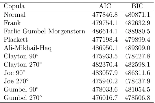
To simplify the process, we exploited the fact that in a copula context the specification of margins and copula can be viewed as separate but related issues. We first chose the marginal distributions based on the AIC and BIC values (see Table 1). Then we moved on to the choice of copula. Specifically, we started off with the Gaussian and then, based on the (negative or positive) sign of the dependence, we tried out the alternative specifications that were consistent with this initial finding. In this case, the values for the correlation coefficients were found to be negative. Therefore, we only considered copula which were consistent with this sign of dependence (see Table 2).
Y1: low birth weight Y2: gestational age
Distribution AIC BIC AIC BIC
Normal 52816.28 53249.79 466124.1 468094.7
Gumbel 52833.92 53273.13 440225.2 441942.9
Reverse Gumbel - - 518570.4 520754.7
Logistic 52828.86 53267.76 452021.4 453842.5
Log-normal - - 473938.8 475957.8
Weibull - - 441611.7 443345.4
Inverse Gaussian - - 473678.4 475678.2
Gamma - - 500382.1 501186.1
Dagum - - 439730.9 441992.1
Singh-Maddala - - 3526100 3526607
[image:14.595.124.452.127.321.2]Fisk - - 457351.8 457907.3
Table 1: Comparison of AIC and BIC values for the candidate marginal distribu-tions for low birth weight and gestational age. For the binary response, only the classical link functions resulting from assuming the Gaussian, Gumbel and logistic distributions were considered, hence the dash symbols for the other distributions.
Copula AIC BIC
Normal 477846.8 480871.1
Frank 479754.1 482632.9
Farlie-Gumbel-Morgenstern 486614.1 488980.5
Plackett 477198.4 479899.4
Ali-Mikhail-Haq 486950.1 489309.0
Clayton 90◦ 475933.5 478427.8
Clayton 270◦ 482370.4 482598.1
Joe 90◦ 483057.9 486311.6
Joe 270◦ 475940.2 478437.9
Gumbel 90◦ 478033.6 481054.5
[image:14.595.155.423.511.690.2]Gumbel 270◦ 476016.7 478506.8
eq1 <- lbw ~ male + race + educ + marital + smokes + firstbirth + dobmonth + s(age) + s(county, bs = "mrf", xt = xt) eq2 <- wksgest ~ male + race + educ + marital + smokes + firstbirth +
dobmonth + s(age) + s(county, bs = "mrf", xt = xt) eq3 <- ~ male + race + educ + marital + smokes + firstbirth +
dobmonth + s(age) + s(county, bs = "mrf", xt = xt) eq4 <- ~ male + race + educ + marital + smokes + firstbirth +
dobmonth + s(age) + s(county, bs = "mrf", xt = xt)
f.l <- list(eq1, eq2, eq3, eq4)
outC90 <- gjrm(f.l, margins = c("probit", "GU"), BivD = "C90", Model = "B", data = dat)
where the s(age) are the smooth effects of age represented using thin plate regres-sion splines with 10 basis functions and penalties based on second order derivatives, the s(county, bs = "mrf", xt = xt) represent spatial effects with neighborhood structure information stored inxt, argumentsmarginsandBivDhave the obvious in-terpretations andModel = "B"stands for bivariate model (other options are available in the package).
Using a 2.20-GHz Intel(R) Core(TM) computer running Windows 7, computing time was about 25 minutes for a sample size of n = 109,380 observations and number of parameters equal to 524, hence highlighting the efficiency of the numerical implemen-tation.
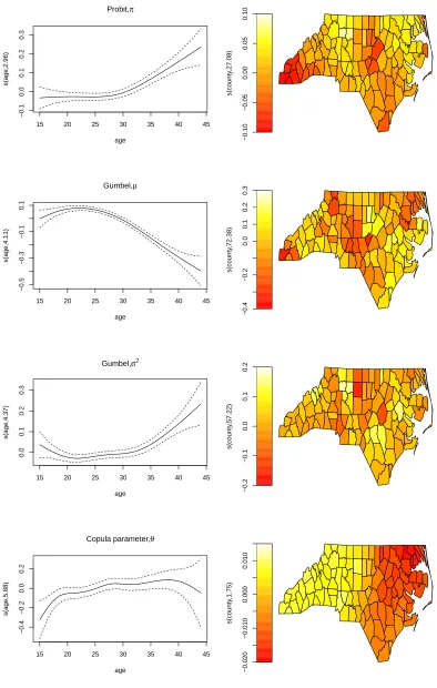
The R summary output in the Appendix presents the regression coefficients from the bivariate model for low birth weight (a binary indicator for being born with a weight less than 2,500 grams), and gestational age (measured in continuous weeks). As outlined above, flexible splines are used to model the association between maternal age and each outcome, and a Markov random field smoother is applied to the county indicators of mother’s residence.
4.1
Results
Effects of Covariates As in Neelon et al. (2014), we find the expected associations
between the covariates and outcomes of interest. As noted previously (Kramer, 1987), some factors have adverse associations with both intrauterine growth and gestational duration, while others contribute positively to one and negatively to the other. For example, male babies are less likely to be low birth weight, but more likely to be born early (by around 2 weeks on average after adjusting for other covariates). First births are born later, but more likely to be underweight. In contrast, the impact of maternal smoking is unambiguously negative. It increases the risk of low birth weight, and reduces gestational age (also by around 2 weeks). The most substantial coefficient for gestational duration in terms of magnitude relates to race. Babies born to black mothers are more likely to be low birth weight, and more likely to be born early (by around 6 weeks). In contrast, babies born to Hispanic mothers are less likely to be low birth weight and more likely to be born later. Education does not appear to have a consistent impact on either outcome.
of spline functions, with the risk of low birth weight increasing after the mid-30s, and gestational age reaching its maximum in the mid-20s.
These results point to both modifiable and non-modifiable risk factors for poor early life health. The main modifiable risk factor is smoking, which emphasises the impor-tance of public health campaigns to reduce smoking prevalence for promoting infant health. Non-modifiable risk factors, such as maternal age, race, and place of residence (county) are also important from a policy perspective because they provide a basis for identifying cohorts and individuals at risk. Because of the adverse consequences associated with low birth weight and early gestational age in both the short and long run (Black et al., 2007; McGovern, 2013), an understanding of who is likely to experience these outcomes can help direct where resources are targeted. Moreover, as we argue above, because of the multiplicative risk of adverse outcomes associated with jointly being preterm and low birth weight, it is important to identify babies in this category. By simultaneously modelling the outcomes under study, and allow-ing for flexible dependence between birth weight and gestational age, the statistical model described in this paper permits estimation of the relevant joint and marginal quantities of interest.
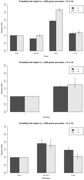
Predicting joint relatives risks Figure 3 shows a bar plot with relative risk ratios
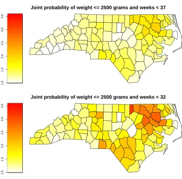
for being low birth and being born before 37 weeks and 32 weeks, stratified by race, maternal smoking status and education. It is apparent from this figure that babies born to black mothers are at greatest risk, with the predicted probability of joint occurrence of LBW and being before 37 weeks of around 8%, roughly twice that of babies of other races. A similar risk penalty is apparent when stratifying by maternal smoking status. Here again the relative risk of joint occurrence of LBW and being born before 37 weeks is almost twice as great for babies born to mothers who smoke compared to mothers who do not. Mothers with higher levels of education appear to have babies who are at greater risk, however the confidence intervals are also wide. In Figure 4 (top), the relative risk of joint occurrence of LBW and being born before 37 weeks are shown by county of residence (of which there are 100) in North Carolina. Risk of an infant being born both LBW and preterm varies widely across counties, with the relative risk of joint occurrence of up to 2 for the highest compared to lowest risk counties of residence, and the absolute prevalence ranging from 3% to 8%. The least favourable places to be born are clustered in the northeast of the state, specifically Hertford, Northampton, Halifax, Warren, Vance, Edgecombe, Bertie, and Washington counties. These results clearly indicate substantial inequality at birth dependent on a number of background characteristics including place of residence, smoking status, and race.
15 20 25 30 35 40 45
−0.1
0.0
0.1
0.2
0.3
Probit,π
age
s(age
,2.96)
−0.10
−0.05
0.00
0.05
0.10
s(county
,27.08)
15 20 25 30 35 40 45
−0.5
−0.3
−0.1
0.1
Gumbel,µ
age
s(age
,4.11)
−0.4
−0.2
0.0
0.1
0.2
0.3
s(county
,72.38)
15 20 25 30 35 40 45
0.0
0.1
0.2
0.3
Gumbel,σ2
age
s(age
,4.37)
−0.2
−0.1
0.0
0.1
0.2
s(county
,57.22)
15 20 25 30 35 40 45
−0.4
−0.2
0.0
0.2
Copula parameter,θ
age
s(age
,5.88)
−0.020
−0.010
0.000
0.010
s(county
[image:17.595.86.480.78.698.2],1.75)
White Hispanic Black Other < 37 < 32
Probability that weight is =< 2500 grams and weeks < 37 or 32
Race
Relativ
e Risk
0.0
0.5
1.0
1.5
2.0
2.5
3.0
0 1
< 37
< 32
Probability that weight is =< 2500 grams and weeks < 37 or 32
Smokes
Relativ
e Risk
0.0
0.5
1.0
1.5
2.0
2.5
3.0
Primary Secondary Tertiary
< 37 < 32 Probability that weight is =< 2500 grams and weeks < 37 or 32
Education
Relativ
e Risk
0.0
0.5
1.0
1.5
2.0
2.5
[image:18.595.152.423.70.650.2]3.0
Figure 3: Joint probabilities for being low birth and being born before 37 weeks and 32 weeks by race, smoking behavior and education. The results are presented in terms of relative risk ratios where the baseline categories are white, non-smoker and primary, respectively. Variable age was set to its average, whereas the other factor variables were set to the respective categories with highest frequencies.
1.0
1.5
2.0
2.5
3.0
3.5
Joint probability of weight <= 2500 grams and weeks < 37
1.0
1.5
2.0
2.5
3.0
3.5
[image:19.595.101.468.64.426.2]Joint probability of weight <= 2500 grams and weeks < 32
Figure 4: Joint probabilities for being low birth and being born before 37 weeks and 32 weeks by county of residence. The results are displayed in terms of relative risk ratios where the baseline counties are those exhibiting the lowest probabilities.
from our statistical model for being born low birth weight and gestational age less than 32 weeks. This allows us to predict the characteristics of babies among whom risk of mortality is most concentrated. The second set of bars in Figure 3 show these results for maternal race, smoking, and education. It is apparent that being born to a black mother is again an increased risk factor, however in this case the relative risk is even greater than for being born before 37 weeks. Compared to white mothers, babies born to black mothers are 2.75 times more likely to be low birth weight and fall below the 32 week cut-off, as opposed to 2 times more likely to be low birth weight and be born before 37 weeks. This suggests that racial inequality is even greater than would be expected from examining the standard 37 week cut-off. This same pattern for being born before 32 weeks in relation to county of residence is apparent from Figure 4 (bottom), with higher relative risk ratios than for 37 weeks. The same counties exhibit the highest risk, but in this case babies in these locations are up to 3 times more likely to fall below the relevant cut-offs.
Conditional dependence of outcomes Figure 5 shows the estimates for
−0.31
−0.30
−0.29
−0.28
−0.27
−0.26
[image:20.595.102.476.74.241.2]Kendall’s τ^
Figure 5: Estimates for Kendall’s τ obtained using the 90 degrees Clayton model. These have been averaged by the covariate values, within each county in North Carolina.
and heterogeneous across counties. This clearly supports the presence of dependence between the binary and continuous outcomes, after accounting for covariates, and hence that prediction of the relative risks has to be based on the joint model rather than the marginal ones.
Our overall estimate for the association between low birth weight and gestational age is negative (the copula parameter is estimated to be−0.296 (95% CI−0.323,−0.271) indicating that those who are low birth weight are more likely to be born earlier. However, our model allows us to examine whether this expected negative dependence is modified by the covariates we include. For example, male babies exhibit less strong dependence (the relevant parameter in the equation for the dependence parameter is negative), as do babies born to black mothers and mothers with tertiary education. This finding is relevant because it indicates that those in these categories are more able to break the link between the two outcomes, and are less likely to suffer the double disadvantage of being both low birth weight and early for gestational age. In contrast, babies born to mothers of Hispanic origin, or mothers who smoke, exhibit even more negative dependence, indicating that if the baby is low birth weight they are also more likely to be born early.
5
Discussion
We have developed an inferential framework for fitting flexible bivariate regression copula models with binary and continuous margins with the aim of examining the risk factors of adverse birth outcomes. Parameter estimation is carried out within a penalized maximum likelihood estimation framework with integrated automatic multiple smoothing parameter selection, and the proposed model can be easily used via the R package GJRM.
example, as we discussed in relation to infant mortality. Our results have a number of policy implications. First, we identify substantial racial inequalities in that babies born to black mothers are more than twice as likely to be low birth weight and be born earlier than babies born to mothers of other races. In addition, these disparities are also evident across county of residence, whereby the relative risk of joint occur-rence for the worst counties is around twice that of the best counties. Second, we find that these disparities get worse across the gestational age distribution, and not just for the preterm cut-off of before 37 weeks. Given the concentration in mortal-ity before 32 weeks of gestation, this is likely to be the group most appropriate for policy intervention. Confirmation of these racial and spatial inequalities in early life health may provide a basis for action to target these disparities. Given the evidence supporting the short and long run impact of initial conditions, this is likely to be a policy priority (Deaton, 2013). In addition to the covariates examined here, the model is more widely applicable because it can be used to flexibly model both the impact of other covariates of interest (including non-linearity in continuous predictors and spatial dependence), and other outcomes of interest, one of which is binary and one of which is continuous, which are expected to be correlated.
References
Acar, E. F., Craiu, V. R. and Yao, F. (2013). Statistical testing of covariate effects in conditional copula models,Electronic Journal of Statistics7: 2822–2850.
Almond, D. and Currie, J. (2011). Killing Me Softly: The Fetal Origins Hypothesis, The Journal of Economic Perspectives25: 153–172.
Behrman, J. R. and Rosenzweig, M. R. (2004). Returns to birthweight,Review of Economics and Statistics86: 586–601.
Black, S. E., Devereux, P. J. and Salvanes, K. G. (2007). From the Cradle to the La-bor Market? The Effect of Birth Weight on Adult Outcomes,The Quartely Journal of Economics122: 409–439.
Deaton, A. (2013). What does the empirical evidence tell us about the injustice of health inequalities?,inE. Nir, S. Hurst, O. Norheim and D. Wiclker (eds),Inequalities in health: concepts measures, and ethics, Oxford University Press, Oxford, pp. 263–281.
Eilers, P. H. C. and Marx, B. D. (1996). Flexible smoothing with B-splines and penalties, Statistical Science11: 89–121.
Fahrmeir, L., Kneib, T. and Lang, S. (2004). Penalized structured additive regression for space-time data: A Bayesian perspective,Statistica Sinica14: 731–761.
Fahrmeir, L., Kneib, T., Lang, S. and Marx, B. (2013). Regression - Models, Methods and Applications, Springer, Berlin.
Gijbels, I., Veraverbeke, N. and Omelka, M. (2011). Conditional copulas, association mea-sures and their applications,Computational Statistics & Data Analysis 55: 1919–1932.
Hediger, M. L., Overpeck, M. D., Ruan, W. J. and Troendle, J. F. (2002). Birthweight and gestational age effects on motor and social development, Paediatric and Perinatal Epidemiology16: 33–46.
Joe, H. (1997). Multivariate Models and Dependence Concepts, Chapman & Hall/CRC, London.
Kauermann, G., Schellhase, C. and Ruppert, D. (2013). Flexible copula density estimation with penalized hierarchical b-splines,Scandinavian Journal of Statistics40: 685–705.
Klein, N. and Kneib, T. (2016). Simultaneous estimation in structured additive condi-tional copula regression models: A unifying Bayesian approach,Statistics and Computing
26: 841–860.
Kraemer, N. and Silvestrini, D. (2015). CopulaRegression: Bivariate Copula Based Regres-sion Models. R package verRegres-sion 0.1-5.
URL:http://CRAN.R-project.org/package=CopulaRegression
Kramer, M. S. (1987). Intrauterine growth and gestational duration determinants, Pedi-atrics80: 502–511.
Kramer, N., Brechmann, E. C., Silvestrini, D. and Czado, C. (2012). Total loss estimation using copula-based regression models,Insurance: Mathematics and Economics53: 829–
839.
Lambert, P. (2007). Archimedean copula estimation using bayesian splines smoothing tech-niques,Computational Statistics & Data Analysis51: 6307–6320.
Marra, G. and Radice, R. (2017a). Bivariate copula additive models for location, scale and shape,Computational Statistics and Data Analysis 112: 99–113.
Marra, G. and Radice, R. (2017b). GJRM: Generalised Joint Regression Modelling. R package version 0.1-4.
URL:http://CRAN.R-project.org/package=GJRM
Marra, G., Radice, R., B¨arnighausen, T., Wood, S. N. and McGovern, M. E. (2017). A simultaneous equation approach to estimating HIV prevalence with non-ignorable missing responses,Journal of the American Statistical Association12: 484–496.
Marra, G. and Wood, S. (2012). Coverage properties of confidence intervals for generalized additive model components,Scandinavian Journal of Statistics39: 53–74.
McGovern, M. E. (2013). Still unequal at birth: birth weight, socio-economic status and outcomes at age 9,The Economic and Social Review44: 53–84.
Neelon, B., Anthopolos, R. and Miranda, M. L. (2014). A spatial bivariate probit model for correlated binary data with application to adverse birth outcomes,Statistical Methods in Medical Research23: 119–133.
Nelsen, R. (2006). An Introduction to Copulas, New York: Springer.
Nocedal, J. and Wright, S. J. (2006). Numerical Optimization, New York: Springer-Verlag.
Radice, R., Marra, G. and Wojtys, M. (2016). Copula regression spline models for binary outcomes,Statistics and Computing 26: 981–995.
Rigby, R. A. and Stasinopoulos, D. M. (2005). Generalized additive models for location, scale and shape (with discussion), Journal of the Royal Statistical Society, Series C
54: 507–554.
Rue, H. and Held, L. (2005). Gaussian Markov Random Fields, Chapman & Hall/CRC, New York/Boca Raton.
Ruppert, D., Wand, M. P. and Carroll, R. J. (2003).Semiparametric Regression, Cambridge University Press, New York.
Sabeti, A., Wei, M. and Craiu, R. V. (2014). Additive models for conditional copulas, Stat
3: 300–312.
Segers, J., van den Akker, R. and Werker, B. J. M. (2014). Semiparametric Gaussian copula models: Geometry and efficient rank-based estimation, Annals of Statistics 42: 1911–
1940.
Shen, X., Zhu, Y. and Song, L. (2008). Linear B-spline copulas with applications to nonpara-metric estimation of copulas,Computational Statistics & Data Analysis 52: 3806–3819.
Silverman, B. W. (1985). Some aspects of the spline smoothing approach to non-parametric regression curve fitting,Journal of the Royal Statistical Society Series B47: 1–52.
Slattery, M. M. and Morrison, J. J. (2002). Preterm delivery,The Lancet 360: 1489–1497.
Vatter, T. and Chavez-Demoulin, V. (2015). Generalized additive models for conditional dependence structures,Journal of Multivariate Analysis 141: 147–167.
Wardlaw, T., Blanc, A., Zupan, J. and Ahman, E. (2005). United Nations Children’s Fund and World Health Organization, Low Birthweight: Country, Regional and Global Estimates.
Wojtys, M. and Marra, G. (2015). Copula based generalized additive models with non-random sample selection,arXiv:1508.04070 .
Wood, S. N. (2004). Stable and efficient multiple smoothing parameter estimation for generalized additive models, Journal of the American Statistical Association 99: 673–
686.
Wood, S. N. (2006). Generalized Additive Models: An Introduction With R, Chapman & Hall/CRC, London.
Wood, S. N. (2013a). On p-values for smooth components of an extended generalized additive model,Biometrika 100: 221–228.
Wood, S. N. (2013b). A simple test for random effects in regression models, Biometrika
100: 1005–1010.
Yan, J. (2007). Enjoy the joy of copulas: With a package copula, Journal of Statistical Software21: 1–21.
Appendix
Summary of parametric and non-parametric effects from the 90 degrees rotated Clayton copula model with Bernoulli (with probit link) and Gumbel margins. Sample size is 109380, whereas the overal estimate for θ with CI is −0.847(−0.96,−0.749). The corresponding Kendall’s tau is −0.296(−0.323,−0.271). Total number of effective degrees of freedom is 260.
COPULA: 90 Clayton MARGIN 1: Bernoulli MARGIN 2: Gumbel
EQUATION 1
Link function for mu.1: probit
Formula: lbw ~ male + race + educ + marital + smokes + firstbirth + dobmonth + s(mage, k = 12, bs = "ps", m = c(2, 2)) + s(county, bs = "mrf",
xt = xt)
Parametric coefficients:
Estimate Std. Error z value Pr(>|z|) (Intercept) -1.569347 0.045614 -34.405 < 2e-16 *** male1 -0.089513 0.011734 -7.629 2.38e-14 *** raceHispanic -0.059786 0.021324 -2.804 0.00505 ** raceBlack 0.339162 0.015379 22.053 < 2e-16 *** raceOther 0.169090 0.028753 5.881 4.08e-09 *** educSecondary 0.070154 0.038956 1.801 0.07172 . educTertiary -0.033780 0.040390 -0.836 0.40296 marital1 -0.101551 0.014805 -6.859 6.93e-12 *** smokes1 0.352365 0.018065 19.506 < 2e-16 *** firstbirth1 0.106756 0.013304 8.025 1.02e-15 *** dobmonth2 -0.039269 0.029054 -1.352 0.17650 dobmonth3 -0.004533 0.028483 -0.159 0.87354 dobmonth4 -0.015908 0.029016 -0.548 0.58352 dobmonth5 -0.009279 0.028750 -0.323 0.74690 dobmonth6 0.010851 0.028527 0.380 0.70366 dobmonth7 -0.016584 0.028284 -0.586 0.55765 dobmonth8 -0.018836 0.028315 -0.665 0.50590 dobmonth9 -0.037382 0.028612 -1.307 0.19138 dobmonth10 -0.007949 0.028268 -0.281 0.77856 dobmonth11 -0.034410 0.029093 -1.183 0.23690 dobmonth12 0.013941 0.028166 0.495 0.62063
---Signif. codes: 0 *** 0.001 ** 0.01 * 0.05 . 0.1 1
Smooth components’ approximate significance: edf Ref.df Chi.sq p-value s(mage) 2.964 3.664 54.91 6.05e-11 *** s(county) 27.079 99.000 61.36 2.61e-07 ***
EQUATION 2
Link function for mu.2: identity
Formula: wksgest ~ male + race + educ + marital + smokes + firstbirth + dobmonth + s(mage, k = 12, bs = "ps", m = c(2, 2)) + s(county, bs = "mrf", xt = xt)
Parametric coefficients:
Estimate Std. Error z value Pr(>|z|) (Intercept) 39.613609 0.035462 1117.058 < 2e-16 ***
male1 -0.073412 0.009735 -7.541 4.67e-14 ***
raceHispanic 0.034584 0.016479 2.099 0.035839 * raceBlack -0.317929 0.014651 -21.700 < 2e-16 *** raceOther -0.082286 0.024253 -3.393 0.000692 *** educSecondary -0.035389 0.029332 -1.207 0.227620 educTertiary 0.031329 0.030589 1.024 0.305742 marital1 -0.003031 0.012776 -0.237 0.812469 smokes1 -0.110066 0.018665 -5.897 3.70e-09 *** firstbirth1 0.221671 0.011081 20.004 < 2e-16 *** dobmonth2 -0.017297 0.024262 -0.713 0.475882 dobmonth3 -0.008670 0.024012 -0.361 0.718048 dobmonth4 0.023724 0.024190 0.981 0.326722 dobmonth5 -0.027441 0.023975 -1.145 0.252391 dobmonth6 -0.037190 0.023954 -1.553 0.120527 dobmonth7 0.017129 0.023580 0.726 0.467591 dobmonth8 0.008875 0.023343 0.380 0.703799 dobmonth9 0.072997 0.023279 3.136 0.001714 ** dobmonth10 0.022596 0.023598 0.958 0.338300 dobmonth11 0.030304 0.024061 1.259 0.207865 dobmonth12 0.015868 0.023954 0.662 0.507696
---Signif. codes: 0 *** 0.001 ** 0.01 * 0.05 . 0.1 1
Smooth components’ approximate significance: edf Ref.df Chi.sq p-value
s(mage) 4.108 4.983 307.7 <2e-16 *** s(county) 72.382 99.000 586.4 <2e-16 ***
---Signif. codes: 0 *** 0.001 ** 0.01 * 0.05 . 0.1 1
EQUATION 3
Link function for sigma2: log
Formula: ~male + race + educ + marital + smokes + firstbirth + dobmonth + s(mage, k = 12, bs = "ps", m = c(2, 2)) + s(county, bs = "mrf",
xt = xt)
Parametric coefficients:
Estimate Std. Error z value Pr(>|z|) (Intercept) 0.878581 0.033827 25.973 < 2e-16 ***
male1 0.045561 0.009311 4.893 9.91e-07 ***
raceOther 0.068929 0.023282 2.961 0.003070 ** educSecondary 0.010272 0.027917 0.368 0.712896 educTertiary -0.103331 0.029156 -3.544 0.000394 *** marital1 -0.105515 0.011945 -8.833 < 2e-16 *** smokes1 0.147066 0.016612 8.853 < 2e-16 *** firstbirth1 -0.013728 0.010693 -1.284 0.199198 dobmonth2 0.021599 0.022993 0.939 0.347551 dobmonth3 0.027197 0.022744 1.196 0.231768 dobmonth4 0.020124 0.022993 0.875 0.381470 dobmonth5 0.011315 0.022893 0.494 0.621148 dobmonth6 0.009636 0.022781 0.423 0.672307 dobmonth7 0.010346 0.022458 0.461 0.645017 dobmonth8 -0.027985 0.022339 -1.253 0.210293 dobmonth9 -0.061163 0.022553 -2.712 0.006689 ** dobmonth10 -0.008476 0.022602 -0.375 0.707643 dobmonth11 -0.023756 0.023012 -1.032 0.301910 dobmonth12 0.027743 0.022658 1.224 0.220802
---Signif. codes: 0 *** 0.001 ** 0.01 * 0.05 . 0.1 1
Smooth components’ approximate significance: edf Ref.df Chi.sq p-value
s(mage) 4.37 5.278 57.32 9.25e-11 *** s(county) 57.22 99.000 351.06 < 2e-16 ***
---Signif. codes: 0 *** 0.001 ** 0.01 * 0.05 . 0.1 1
EQUATION 4
Link function for theta: log(- )
Formula: ~male + race + educ + marital + smokes + firstbirth + dobmonth + s(mage, k = 12, bs = "ps", m = c(2, 2)) + s(county, bs = "mrf",
xt = xt)
Parametric coefficients:
Estimate Std. Error z value Pr(>|z|) (Intercept) -0.443353 0.106572 -4.160 3.18e-05 ***
male1 0.055999 0.026091 2.146 0.031851 *
dobmonth8 0.153894 0.064453 2.388 0.016955 * dobmonth9 0.009381 0.064231 0.146 0.883881 dobmonth10 -0.004853 0.063891 -0.076 0.939453 dobmonth11 -0.003268 0.065797 -0.050 0.960393 dobmonth12 0.093968 0.063081 1.490 0.136319
---Signif. codes: 0 *** 0.001 ** 0.01 * 0.05 . 0.1 1
Smooth components’ approximate significance: edf Ref.df Chi.sq p-value
s(mage) 5.878 6.912 19.983 0.0071 ** s(county) 1.752 99.000 2.219 0.1817
---Signif. codes: 0 *** 0.001 ** 0.01 * 0.05 . 0.1 1
n = 109380 sigma2 = 2.43(2.26,2.61)