City, University of London Institutional Repository
Citation
:
Buckney, D., Kovacevic, A. & Stosic, N. (2016). Design and evaluation of rotor clearances for oil-injected screw compressors. Proceedings of the Institution of Mechanical Engineers, Part E: Journal of Process Mechanical Engineering, 231(1), pp. 26-37. doi: 10.1177/0954408916660342This is the accepted version of the paper.
This version of the publication may differ from the final published
version.
Permanent repository link:
http://openaccess.city.ac.uk/15243/Link to published version
:
http://dx.doi.org/10.1177/0954408916660342Copyright and reuse:
City Research Online aims to make research
outputs of City, University of London available to a wider audience.
Copyright and Moral Rights remain with the author(s) and/or copyright
holders. URLs from City Research Online may be freely distributed and
linked to.
City Research Online: http://openaccess.city.ac.uk/ publications@city.ac.uk
Design and evaluation of rotor clearances for oil injected screw compressors
David Buckney1, Ahmed Kovacevic2, Nikola Stosic2
1. Howden Compressors Ltd., R&D 2. City University, Centre for Compressor Technology
Email: david.buckney@howden.com
Abstract
Designing twin screw compressors to safely operate at higher than normal temperatures poses a challenge as
the compressor must accommodate larger peak thermal distortions while maintaining efficiency at nominal
operating conditions. This paper will present a case study of an oil injected compressor tested at elevated
discharge temperatures with original and revised clearances. A procedure is presented to use boundary
conditions derived from a chamber model to approximate component temperature distributions that are then
used to predict possible thermal distortions and the resulting effect on clearance gaps. The original and revised
clearance designs are evaluated and performance penalties incurred due to the modifications are discussed.
Keywords
Twin screw compressor; boundary map; rotor temperature; thermal distortion; clearances
Notation
A centre distance between rotor axes
G clearance gap
L, l length
n integer
r polar co-ordinate radius
S co-ordinate system origin
s line parameter
X, x Cartesian co-ordinate Y, x Cartesian co-ordinate
Z, z Cartesian co-ordinate / number of rotor lobes
β non-standard polar co-ordinate angle
γ local wrap angle
ε rotor surface parameter
θ cycle angle
λ transverse profile offset angle
φ polar co-ordinate angle / various angles
Subscripts
1 main (male) rotor
2 gate (female) rotor
c cusp angle
I interlobe
M meshing angle
s start
R rotor
B casing bore
w wrap angle
local local cycle angle
Introduction
End users of twin screw compressors occasionally demand reliable compressor operation over a greater
operating range than the original design envelope. If for example the allowable cooling oil temperature can be
increased, this can reduce the cooling requirements and the overall plant cost. This poses a challenge as the
compressor design needs to accommodate higher peak operating temperatures while maintaining efficiency at
In one sense the clearances in oil injected machines are easier to manage than in oil free machines as
temperatures are usually kept within much lower limits however the lack of timing gears and the direct rotor to
rotor contact does add more complexity to clearance analysis. Rotor contact is of course necessary for one
rotor to drive the other; the objective is to control precisely where it is possible for contact to occur. Best
practice for direct drive clearance design ensures only rolling contact at the pitch radius of each rotor as
presented by Stosic et al [1]. Deviations from nominal design clearances, whether due to manufacturing and
assembly variations or due to operational distortions can result in a shift in the relative rotation between the
main and gate rotors [2]: this further distorts the interlobe clearance distribution and must be considered in
clearance evaluation for direct drive, oil injected compressors.
This paper will present a case study of an oil injected compressor that was tested at elevated discharge
temperatures. A novel procedure is presented to estimate local clearance distortions by applying boundary
conditions derived from a quasi 1-dimensional chamber model. A key stage in this procedure is the creation of
a ‘Rotor Boundary Map’ which is unique for any given profile. The Rotor Boundary Map allows rotor to rotor
and rotor to casing boundaries to be visualized on a single 2-dimensional map which allows the interaction
between various compression chambers to be investigated.
Time varying boundary conditions from the non-dimensional model are mapped onto rotor and casing
surfaces. The fluid boundary temperatures are time-averaged then used to estimate the local rotor and casing
temperatures. Rather than apply these boundary conditions to finite element analysis [3], the thermal and
clearance analysis takes a more direct analytical approach that requires some carefully considered
assumptions. Heat transfer assumptions that represent the extreme case for component temperature
distributions are presented. This is then used to predict possible thermal distortions and the resulting affect on
Mapping fluid properties
Co-ordinate system
Figure 1 shows a representation of the casing bores and rotor axes for a twin screw machine. The global
ordinate system, S(X,Y,Z), is located on the main rotor axis and the high pressure (HP) plane. Two additional
co-ordinate systems, S1(x1,y1,z1) and S2(x2,y2,z2) have been located on the low pressure (LP) plane on the main and
gate rotor axes respectively. This convention can be applied to any screw compressor or expander providing
[image:5.595.73.526.335.682.2]the helix on the main rotor is left handed.
With the cylindrical form of the rotor bores and the rotational movement of the rotors it is convenient to
define points using a cylindrical co-ordinate systems located at the origins S1 and S2. In the standard convention
for a polar co-ordinate system, (r,θ,z), the angle θ is measured counter-clockwise from the x axis and z is in the
direction already defined. To simplify later equations it is preferable to define less conventional angle
parameters that are aligned with the direction of rotation for each respective rotor. In addition it is easier to
use an axial length parameter that is aligned from the compressor inlet to outlet. Parameters r, β and l have
been defined on each co-ordinate system S1 and S2 as shown in Figure 1. r is the local radius, β is the angle
,measured in the same direction that the rotors rotate, and l is a measure of the axial position from compressor
inlet. The length, l, can alternatively be defined by using an angular parameter, γ; this describes the local wrap
angle measured from the compressor inlet. For the case of rotors with constant pitch helix the relationship is as
shown in equation (1) where φw1 is the main rotor wrap angle over the rotor length, l. The parameter γ always
refers to the main rotor wrap angle. Equations (2) to (4) describe transformations from these parameters, back
to the global Cartesian compressor system located at S.
𝑙𝑙 𝐿𝐿
=
𝛾𝛾
𝜑𝜑𝑤𝑤1 (1)
𝑋𝑋= 𝑟𝑟1𝑐𝑐𝑐𝑐 𝑠𝑠(𝛽𝛽1) = −𝑟𝑟2𝑐𝑐𝑐𝑐𝑠𝑠(𝛽𝛽2) + 𝐴𝐴 (2) 𝑌𝑌= −𝑟𝑟1𝑠𝑠𝑠𝑠 𝑛𝑛(𝛽𝛽1) = −𝑟𝑟2𝑠𝑠𝑠𝑠𝑛𝑛 (𝛽𝛽2) (3)
𝑍𝑍= 𝐿𝐿 �1−𝜑𝜑γ
𝑤𝑤1�= 𝐿𝐿 �1−
γ
𝜑𝜑𝑤𝑤1� (4)
Rotor surfaces
Each rotor surface is replaced by a 2D surface, represented by a 2D array. The transformation between the 3D
spatial domain of a rotor surface and the 2D surface computational domain is done by utilising the co-ordinate
systems explained. The full 3-dimensional surface of the rotors in Figure 2 can be derived using the transverse
co-ordinate system: S01(x01,y01); which is fixed to the main rotor as illustrated in Figure 3. The main rotor is only
partially constrained to co-ordinate system S1(x1,y1,z1) as it can freely rotate about its axis, z1. An instantaneous
point on this rotor surface could be represented globally using (X,Y,Z); or local to the respective rotor bore on
origin S1 using (x1,y1,z1) or with parameters (r1,β1,γ1). The advantage of using the latter is that parameters, γ1
and r1 are constant, however the angle, β1, is affected by the rotational position of the rotor, defined by the
[image:7.595.74.488.316.611.2]cycle angle, θ.
Figure 2: Full surface of main rotor
An array has been defined to identify a surface location on a single main rotor ridge; or in the case of the gate
rotor, the corresponding flute. This array can be thought of as the surface produced by straightening out the
position along the rotors and the parameter ε represents the position around the contour of the transverse
[image:8.595.87.469.217.537.2]profile.
Figure 3: Rotor surface arrays
𝑠𝑠1= ∫ �𝑑𝑑𝑑𝑑𝐴𝐴𝐵𝐵 012 +𝑑𝑑𝑑𝑑012 (5)
In Figure 3 the length of a curve, s1, between points A and B can be described using equation (5). The
parameter, ε, is defined as the relative position along the line, s, of the transverse rotor profile curve such that
ε varies: 0 ≤ ε ≤ 1. This is defined separately for the main and gate rotor segments. This allows any location on
coordinate systems S01(x01,y01) and S02(x02,y02) can be described using the corresponding polar co-ordinates
(r01,φ01) and (r02,φ02). These points are transverse profile constants that have a unique value for every surface
position described by ε1 or ε2.
Cycle conventions
𝛽𝛽1= (𝜃𝜃 − γ) + (−𝜑𝜑01)− 𝜑𝜑1𝑠𝑠 (6)
𝛽𝛽2= (𝜃𝜃 − γ)𝑧𝑧1𝑧𝑧2 + (𝜑𝜑02− 𝜋𝜋)− 𝜑𝜑2𝑠𝑠 (7)
Equations (6) and (7) define the relationship between the angular position of a point on the rotor surface, β,
and the compression cycle angle, θ. This defines how the geometry will change with time. The parameter γ,
which is related to the axial position, offsets the angle to correct for the rotor helix. Since θ and γ are
referenced to the main rotor, the equation for the gate rotor contains a correction for the gear ratio. The
angles φ01 and φ02 are from the polar co-ordinates that describe a given point on the transverse profile. Finally,
an offset is required to move the rotors to the start position when θ = 0. The offsets φ1s and φ2s are constants
for the main and gate rotors respectively. The offset is defined by the rotation of co-ordinate system S01 with
Figure 4: Main rotor offset to the start position
Rotor boundary map
On the rotor surfaces, the chamber boundaries are defined by the rotor to casing (radial sealing lines) and the
rotor to rotor (interlobe sealing line). Figure 5 shows a transverse cross section of the compressor. For most of
the chambers in this cross-section, the entire rotor flute (or interlobe area) is exposed to the same chamber
which is separated from adjacent chambers by the radial rotor to casing sealing. During rotor to rotor contact
up to three sealing points will be formed between the rotors. When this transverse section is extended to form
Figure 5: Transverse rotors showing boundary points
The ‘Rotor Boundary Map’ shown in Figure 6 is simply a way of abstracting the 3-dimensional chamber sealing
boundaries in order to show what boundaries points occur around one section of the transverse rotor surface
from A (ε1 = 0) to B (ε1 = 1) for a given position of the transverse rotor profile. The position on the rotor surface,
ε, is plotted along the horizontal axis. The parameter, λ, that describes the rotor position, is plotted along the
vertical axis; this parameter is detailed in Figure 5 - note that the convention for this parameter is such that the
Figure 6: Rotor boundary map for main rotor
The boundaries on this map are created by plotting the radial and interlobe sealing lines with respect to ε and
λ. This shows at precisely what rotor position the different boundaries come into play. The rotor to rotor
boundary for the interlobe sealing line is plotted onto the boundary map by setting the profile rotation
parameter λ to equal the profile meshing angle θM. This meshing angle is calculated for any given point of the
transverse profile using the profile curve and gradient [1], [4]. The rotor to casing boundary will always occur at
the same position on the profile, i.e. at the tip of the rotor; resulting in vertical lines on the boundary map. The
limits of this boundary depend on the interaction between the rotor tip and the casing. In Figure 6 this
boundary comes into effect when λ < -φc1 or λ > φc1; where φc1 is the angle to the casing cusp measured from
the main rotor.
There will be a unique boundary map for the main and the gate rotors; the form of the boundaries depends
only on the transverse rotor profiles. This presentation of the rotor boundaries provides a unique way of
this boundary map is that the rotor to rotor boundary does not meet the rotor to casing boundary. This
discontinuity is typical of most practical rotor profile designs and results in what is known as the blow hole
leakage path. In order to explicitly define the distinct compression chambers on this map it is necessary to
introduce an artificial boundary – this was simply created by interpolating between the known boundary
conditions as shown in Figure 8: Rotor boundary map for main rotor. Four distinct quadrants, C1 to C4, have
now been identified that represent different compression ‘chambers’ on the boundary map. This allows the
rotor boundary map to be used as a reference to identify cycle exposure on the rotor surface.
Cycle exposure on surfaces
The actual boundaries that define exposure to different compression chambers are constantly shifting in time
as the rotors rotate. A procedure is needed to identify the location of the boundaries and the chamber
exposure for any given cycle angle. Equations (6) and (7) can be re-arranged in order to calculate the parameter
λ as in equations (8) and (9). For a given cycle angle, the value of λ varies when moving axially along the rotors
due to the rotor helix, described by the parameter γ. In the case of the gate rotor described by the parameters
in equation (9), λ is referenced to the rotational position of the main rotor, similarly to the way the cycle angle
θ is only referenced to the main rotor. In order to use the rotor chamber boundary map the offset should lie in
the range: -π < λ < π. To ensure the parameter λ is within this range a correction can be applied where n in an
appropriate positive or negative integer as in equation (10).
λ= 𝛽𝛽1− (−𝜑𝜑01) = (𝜃𝜃 − γ)− 𝜑𝜑1𝑠𝑠 (8)
λ= �𝛽𝛽2− (𝜑𝜑02− 𝜋𝜋)�𝑧𝑧2𝑧𝑧1 = (𝜃𝜃 − γ)− 𝜑𝜑2𝑠𝑠𝑧𝑧2𝑧𝑧1 (9)
𝜆𝜆ʹ= 𝜆𝜆+ 𝑛𝑛2𝜋𝜋 (10)
For a known position of the rotor surface (ε, γ), at a known cycle angle (θ), the value of λ can now be
chamber quadrant (C1, C2, C3 or C4) the point lies in, this defines the ‘chamber offset’ . When interrogating a
specific point on the rotor surface the required variable is actually the ‘local cycle angle’, θlocal. This is distinct
from the ‘cycle angle’ θ which is effectively a ‘reference cycle angle’ because it only defines the cycle angle for
a single ‘reference compression chamber’. The cycle angle θ defines the position of the rotors while the local
cycle angle θlocal defines cycle exposure at a specific point on the rotor surface, in a specific compression
chamber. Referring back to Figure 6, the chamber offsets have been labelled on the rotor boundary map.
Chamber C4 has been set as the reference chamber.
If any adjustment is made to λ using equation (10) it is important to account for this using an additional term
when calculating the local cycle angle. The general equation for calculation of the local cycle angle θlocal for
each chamber quadrant is given in equations (11) to (14). The number added to the subscript refers to the
chamber quadrant on the rotor boundary map such that θlocal_1 is the local cycle angle in quadrant C1.
𝜃𝜃𝑙𝑙𝑙𝑙𝑙𝑙𝑙𝑙𝑙𝑙_1= 𝜃𝜃+ 2𝜋𝜋+ 2𝜋𝜋𝑧𝑧1+ 𝑛𝑛2𝜋𝜋 (11)
𝜃𝜃𝑙𝑙𝑙𝑙𝑙𝑙𝑙𝑙𝑙𝑙_2= 𝜃𝜃+ 2𝜋𝜋+ 𝑛𝑛2𝜋𝜋 (12)
𝜃𝜃𝑙𝑙𝑙𝑙𝑙𝑙𝑙𝑙𝑙𝑙_3= 𝜃𝜃+2𝜋𝜋𝑧𝑧1+ 𝑛𝑛2𝜋𝜋 (13)
𝜃𝜃𝑙𝑙𝑙𝑙𝑙𝑙𝑙𝑙𝑙𝑙_4= 𝜃𝜃+ 𝑛𝑛2𝜋𝜋 (14)
In Figure 7 the local cycle angle, θlocal, has been represented by colour contours. Areas that are the same colour
can be easily identified as individual compression chambers. Remember that the procedure calculates the local
cycle angle over a single rotor flute, as described by the surface in Figure 3. In order to build up the full rotors
the procedure was repeated after advancing the reference cycle angle θ for each lobe:
Figure 7: Local cycle angle plotted on 3D rotors
Some of the tiles used to produce this plot suggest a transition region across the boundary however this is an
artefact introduced by averaging across nodes that fall in different chambers. All computations are done at the
Thermal analysis of clearance distortions
Fluid boundary temperature
The fluid temperature inside the compressor, assumed to be homogeneous throughout any given compression
chamber, can be calculated with the use of well establish chamber models developed for twin screw
compressors [5]. Once the local cycle angle is known at a given location on the rotor surface for a given cycle
angle it is straightforward to map the corresponding instantaneous fluid properties from a chamber model
onto the rotor surfaces. This instantaneous fluid boundary temperature can be described as a function of the
position on the rotor surface and the cycle angle: TR1(ε1,γ,θ). In equation (16) this temperature has been time
averaged by integrating the temperature at each surface location over one full rotation of the rotor. In
equation (17) the temperature over each transverse cross section of the surface has been averaged around the
transverse profile. Once averaged in this way, the fluid boundary temperature for each respective rotor varies
only with axial position along the rotors, described by the parameter γ.
𝑇𝑇𝑅𝑅1∗ (𝜀𝜀1,𝛾𝛾) = 2𝜋𝜋1 ∫ 𝑇𝑇02𝜋𝜋 𝑅𝑅1(𝜀𝜀1,𝛾𝛾,𝜃𝜃) 𝑑𝑑𝜃𝜃 (16)
𝑇𝑇𝑅𝑅1∗∗(𝛾𝛾) = ∫ 𝑇𝑇01 𝑅𝑅1∗ (𝜀𝜀1,𝛾𝛾) 𝑑𝑑𝜀𝜀1 (17)
A procedure for calculation of the instantaneous fluid temperature at a point on the surface of the casing bores
(B1 and B2) can be applied similarly as for the rotors; in this case the chambers are only defined by the radial
sealing boundary, greatly simplifying the procedure. The surface on the bore is described by the parameters β
and γ so the instantaneous fluid boundary temperature at each point on the bores can be described with the
functions: TB1(β1,γ,θ) and TB2(β2,γ,θ). In order to time average the casing exposure the limits of integration
depend where the point is on the casing surface and covers a range defined by the distance between one lobe
and the next: 2π/z1. Equation (19) is used to time average the temperature at the main rotor bore B1. In
equation (19) the temperature has been averaged over a transverse section of both bores B1and B2. The limits
𝑇𝑇𝐵𝐵1∗ (𝛽𝛽1,𝛾𝛾) = ∫𝜃𝜃𝜃𝜃((𝛽𝛽𝛽𝛽11,𝛾𝛾,𝛾𝛾))+2𝜋𝜋 𝑧𝑧1⁄ 𝑇𝑇𝐵𝐵1(𝛽𝛽1,𝛾𝛾,𝜃𝜃) 𝑑𝑑𝜃𝜃 (18)
𝑇𝑇𝐵𝐵1∗∗,𝐵𝐵2(𝛾𝛾) =
∫𝜑𝜑𝐶𝐶1�2𝜋𝜋−𝜑𝜑𝐶𝐶1�𝑇𝑇𝐵𝐵1∗ (𝛽𝛽1,𝛾𝛾) 𝑑𝑑𝛽𝛽1
4(𝜋𝜋−𝜑𝜑𝐶𝐶1) +
∫𝜑𝜑𝐶𝐶2�2𝜋𝜋−𝜑𝜑𝐶𝐶2�𝑇𝑇𝐵𝐵2∗ (𝛽𝛽2,𝛾𝛾) 𝑑𝑑𝛽𝛽2
4(𝜋𝜋−𝜑𝜑𝐶𝐶2) (19)
Heat transfer assumptions
The realism of thermal analysis depends on accurate representation of the compressor geometry as well as
appropriate boundary conditions describing the compressor interactions with its surrounding. This generally
requires the use of 3D numerical methods such as finite element method (FEM). More realism generally comes
at the expense of more complexity with greater computational cost and time. Despite additional complexity,
use of some assumptions or empirical factors [6] is difficult to avoid. The following procedure is not intended to
calculate the actual local temperature on any given component, rather the average fluid boundary
temperatures will be used to provide a good estimation of the maximum temperature that the compressor
components can reach.
Conduction along the axial length of the rotors is neglected. This means there is no heat transfer from the hot
end to the cold end of the rotor and no heat transfer along the rotor shafts to or from the bearings. This results
in a local maximum rotor temperature which is probably higher than the actual maximum. A uniform
temperature is assumed over the transverse section of each component. The component temperature is
assumed to be the same as the average fluid boundary temperature defined in equations (17) and (19).
Approximating thermal distortions
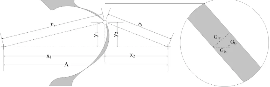
The change in the local interlobe gap is calculated using a 2-dimensional approach. Figure 8 shows the known
location of a local sealing point under investigation. Thermal distortions are evaluated analytically for the: main
rotor co-ordinates x1 and y1; gate rotor co-ordinates x2 and y2; and the distance between axes, A, corrected by
intelobe gap in Figure 8 shows the transverse clearance gap, GIT, and it’s components, GIx and GIy. The change in
the gap is related to changes in the rotor and casing dimensions as described in equations (20) and (21).
Equation (22) states approximations that allow further simplification of the analysis by eliminating the need to
[image:18.595.83.538.271.419.2]use the gate rotor dimensions. Once known, the transverse gap can be used to determine the normal gap [7].
Figure 8: Local definition of intelobe gap
∆GIx= −∆x1 − ∆x2+∆A (20)
∆GIy= �(r1−r1w)
|(r1−r1w)|�(|∆y2| −|∆y1|) (21)
x2 ~ (A−x1); y2 ~ y1 (22)
Case study
Evidence of rotor contact
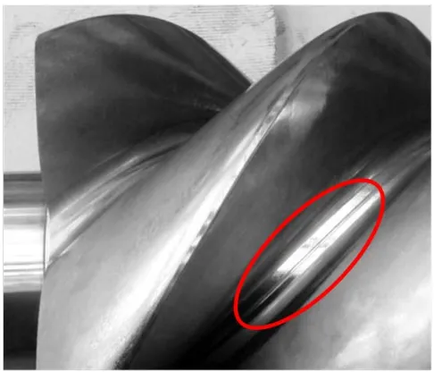
The compressor under investigation is a Howden WCVTA510/193/26; this is currently the largest Howden
compressor with rotors just over 510mm in diameter. In this case the compressor has a built in volume ratio of
2.6. In addition to air testing at the contract pressure ratio and temperature this compressor was tested at an
elevated discharge temperature by increasing the pressure ratio to 11 and then limiting injection oil cooling by
compressor the speed was reduced from the contract speed of 1400rpm to 750rpm during this overload
testing. After testing at up to a discharge temperature of 120°C (from suction at 20°C), tear down inspection
[image:19.595.71.314.243.451.2]revealed that rotor to rotor contact had occurred at the root of the main rotor as highlighted in Figure 9.
Figure 9: Main rotor showing rooting after testing at 120 degrees C
The type of contact observed and the fact that this standard compressor had not presented any problems while
operating within normal temperature limits points to thermal distortion of the rotors being the most likely
cause of this rotor contact. Based on these test findings a revised interlobe clearance design was proposed. The
revised clearance design was implemented on a different compressor at a later date and though teardown
inspection revealed some localised rotor contact, related to the tip sealing strip, there was no contact over the
main part of the root and the clearance modification was approved for further use. To better understand the
clearance behaviour the procedure outlined in this paper was applied to predict component temperatures and
thermal distortions.
The overload test condition, with a discharge temperature of 120° C was modelled to determine how the
temperature varied throughout the compression cycle for that particular duty. All modelling was done to
replicate the test conditions where the overload discharge temperature was achieved by compressing air. The
fluid temperature from the compression cycle was mapped onto the surfaces of the rotors and the casing
bores. Figure 10 shows the temperature of the fluid boundary on the main and gate rotor surfaces. The left
image shows the instantaneous fluid temperature for a particular rotor position. In the right hand image these
[image:20.595.74.526.342.570.2]instantaneous temperatures have been averaged using equations (16) and (17).
Figure 10: Instantaneous (left hand side) and averaged (right hand side) fluid boundary temperature
Table 1: Average fluid boundary temperature across the outlet plane.
Component Description Temperature (°C)
Main rotor 86.8
Gate rotor 73.2
Casing 69.4
[image:20.595.71.383.655.756.2]Figure 10 shows that the peak temperature occurs at the outlet plane of the rotors therefore the analysis will
be based on the average fluid boundary temperatures at outlet; these are presented in Table 1. It is clear that
the averaged fluid boundary temperatures at critical locations on the compressor are actually much lower than
the peak fluid discharge temperature of 120°C.
Clearances
Figure 11 shows the magnitude of normal clearances mapped onto each of the rotors as vectors normal to the
transverse rotor curve. This approach is very intuitive and clearly shows how clearances relate to difference
areas on the rotor profiles, however magnifying the vectors to show the clearance distribution in more detail
quickly distorts the apparent clearance gap due to the curvature of the profiles. On the other hand, plotting
local clearances on a linear axis such as the relative position on the sealing line makes it difficult to determine
[image:21.595.76.514.486.709.2]where the clearances actually occur on the rotors.
Figure 11: Transverse cross-section of main and gate rotors showing local interlobe clearances
A
Figure 12: Interlobe clearance distribution along rack projection of rotors comparing original and revised
[image:22.595.71.456.632.760.2]clearance designs.
Figure 12 shows the clearance distribution in an alternative form where the local clearances are plotted against
a rack projection. Line AB represents the conjugate rack, common to both rotors. The horizontal axis is the arc
length of the rotor pitch circle; this is the axis along which the rack would translate. Vertical lines have been
added along this axis to identify key points along the length of this sealing line projection, details of which are
provided in Table 2. The limits of this rack segment are the beginning and end of the sealing line for a single
compression chamber, as previously highlighted in Figure 11. The secondary axis shows the relative radius on
the rack to give a better indication of where local clearances are located. In this way, the magnitude of the local
clearances can be simply graphed against the somewhat familiar shape of the rack.
Table 2: Key clearance locations
Location on rack Description
A Limit of sealing line for single chamber
1 Pitch circle on the trailing side of the main rotor
2 Root of main rotor / tip of gate rotor
3 Pitch circle on the leading side of the main rotor
0.5 0.6 0.7 0.8 0.9 1.0 0.0 0.2 0.4 0.6 0.8 1.0 1.2 1.4 1.6 1.8 2.0 Re la tiv e ' Ra diu s' Rel at iv e L oc al C lea ra nc e
Relative Position on Rack Projection
Interlobe Clearance Distribution Along Rack Projection of Rotors
Original Clearance Design
Revised Clearance Design
Rack Projection
[image:22.595.73.442.632.759.2]4 Tip of the main rotor / root of the gate rotor
B Limit of sealing line for single chamber
The original and revised clearance distributions are both shown in Figure 12. In all cases the relative rotation
between the rotors is adjusted in order to provide zero clearance at location 3: the pitch radius on the round
side of the rotors. This is where the driving force is transferred from the main to the gate rotor. In the revised
clearance design the main difference is that the clearance in the main rotor root has been increased and to a
lesser extent also at the main rotor tip. Notice that the clearance on the round flank of the rotors (between
locations 3 and 4) has actually been decreased on the revised clearance design – this clearance will not
significantly reduce during operation because the gap is maintained due to the nearby contact at the pitch
point (location 3), therefore this clearance was deemed to be unnecessarily large. Conversely, on the straight
flank (from 4 to B, and from A to 1) the gap is adversely affected by thermal distortions at location 3 which are
transferred over to the straight flank. Therefore it was necessary to increase the clearances on the straight
flank. To quantify how these clearance changes impact the leakage area through the interlobe gap the local
clearances where integrated over the length of the 3D sealing line. The total leakage area is 108.5mm2 for the
original design is and 142.7mm2 for the revised design, an increase of 31.5%.
Clearance distortion results
The following results show the predicted operational clearance distributions for the original and revised
designs in Figure 13 and Figure 14 respectively. The temperature increase in both the rotors and casing shown
in Table 1 would result in little net change in the operational clearances, this case has been presented with the
longer dashed lines on each figure, the trend is not far off the original clearance. A second case has also been
presented where the rotors do not move apart due to casing thermal expansion. This case is likely in the event
end bearings might be situated remotely from the rotor outlet plane in a location where the casing
temperature is much lower than estimated in Table 1. The distance between the two dashed curves for the
different operational scenarios results in a large band of uncertainty but it does serve to highlight 1) where
rotor contact is most likely to occur for a given clearance design, and 2) where clearances can be further
[image:24.595.72.524.296.443.2]reduced without compromising reliability.
Figure 13: Possible variation in interlobe clearance distribution at outlet end (original design)
Figure 14: Possible variation in interlobe clearance distribution at outlet end (revised design)
This analysis supports the suitability of the revised clearance in the root of the main rotor which shows contact
cannot now occur there due to thermal distortion alone. The chance of contact at the tip of the main rotor has
-1.0 -0.8 -0.6 -0.4 -0.20.0 0.2 0.4 0.6 0.8 1.0 1.2 1.4 1.6 1.8 2.0 Rel at iv e L oc al C lea ra nc e
Relative Position on Rack Projection
Possible Variation in Interlobe Clearance Distribution at Outlet End
(Original Design)
Cold Clearance (Design)
Clearance adjusted for potential rotor distortion
Clearance adjusted for potential rotor and casing distortion -1.0 -0.8 -0.6 -0.4 -0.20.0 0.2 0.4 0.6 0.8 1.0 1.2 1.4 1.6 1.8 2.0 Rel at iv e L oc al C lea ra nc e
Relative Position on Rack Projection
Possible Variation in Interlobe Clearance Distribution at Outlet End
(Revised Design)
Cold Clearance (Design)
Clearance adjusted for potential rotor distortion
[image:24.595.75.527.513.663.2]been significantly improved however the analysis suggests contact is still possible under extreme
circumstances.
Performance predictions
The models were also run at the nominal air test duty which is closest to the designed operating conditions:
with a speed of 1400rpm, a pressure ratio of 5 and a discharge temperature maintained at approximately 90°C.
The modelled deviation in the volume flow due to the revised design is compared with the deviation measured
[image:25.595.70.442.390.466.2]on test in Table 3.
Table 3: Performance penalty with revised interlobe clearance at pressure ratio of 5
change in volumetric flow
Modelled -0.5%
Measured on Test -1.7%
The difference between the model result and the test result was higher than expected suggesting that the
model is slightly underestimating the effect of leakages through the interlobe gap. Unfortunately as the test
results were obtained using two different compressors the effect of other manufacturing and assembly
tolerances can’t be ruled out for the test results. Importantly, the resulting change in flow on test was small
enough that the compressor was still within normal operating tolerances in both cases. With the reduced flow
there was a similar reduction in shaft power so there was very little change in the overall efficiency. It is to be
expected there would be some detrimental effect on performance at the nominal operating condition by
increasing the rotor clearances to allow the compressor to operate at higher, non-standard, operating
temperatures. This same design approach could be applied to investigate how far clearances could potentially
Conclusions
A procedure has been presented to map thermodynamic results from a lumped parameter chamber model
onto discrete rotor surfaces. The rotor boundary map used in this procedure provides a unique way of
visualising and comparing the key geometrical properties of different profiles. Fluid boundary conditions
calculated with the aid of the rotor boundary map can be used for further analysis of compressor components.
For example, to provide initial boundary conditions for more specialised finite element analysis (FEA) or
computational fluid dynamics (CFD).
Surface boundary conditions were used to estimate the temperature distribution of the compressor rotors and
casing that result in the largest feasible peak temperatures during normal operation. Local variations in
clearances, due to thermal distortions, have been approximated analytically. This provides valuable data about
where and when in the compression process clearances are inadequate for a given compression application.
Integrating this information into the rotor design process allows a more optimised balance between reliability
and compressor performance.
Two interlobe clearance designs have been analysed to evaluate how suitable they are for operation at an
elevated rotor discharge temperature of 120°C in an oil injected compressor with direct rotor drive. While
there is a fairly large uncertainty on the predicted clearance deviations the results do confirm that the revised
clearances should prevent rotor to rotor contact at the root of the male rotor. This is where contact was
initially present on test, and later shown to be alleviated due to the revised clearance design.
Performance test results suggest that the increase in interlobe clearance has resulted in a 1.7% drop in flow
however the overall flow was still within normal test tolerances. The change in flow predicted by the model
Acknowledgments
The authors would like to thank Howden Compressors Ltd. for supporting this research.
References
1. Stosic N, Smith IK and Kovacevic A. Screw Compressors: Mathematical Modelling and Performance
Calculation. UK. 2005.
2. Sauls J, Powell G, and Weathers B. Thermal deformation effects on screw compressor rotor design. In
International Conference on Compressors and their Systems, September 10, 2007 - September 12, 2007,
pp. 159-168 (Chandos Publishing, London, United kingdom).
3. Sauls J, Powell G, and Weathers B. Transient thermal analysis of screw compressors part I - Development
of thermal model. VDI Berichte , 2006, , 19-29.
4. Litvin FL and Fuentes A. Gear Geometry and Applied Theory. 2004.
5. Hanjalic K and Stosic N. Development and optimization of screw machines with a simulation model - Part
II: thermodynamic performance simulation and design optimization. J Fluids Eng Trans ASME , 1997, 119,
664-670.
6. Hsieh SH, Shih YC, Hsieh W, Lin FY, and Tsai MJ. Calculation of temperature distributions in the rotors of
oil-injected screw compressors. International Journal of Thermal Sciences , 2011, 50, 1271-1284.
7. Holmes C. A study of screw compressor rotor geometry leading to a method for inter-lobe clearance
measurement. Huddersfield Polytechnic. 1990. .