Numerical Simulation of a Passive Control of the Flow Around an Aerofoil Using a Flexible, Self Adaptive Flaplet

City, University of London Institutional Repository

Citation

: Rosti, M. E., Omidyeganeh, M. ORCID: 0000-0002-4140-2810 and Pinelli, A.

ORCID: 0000-0001-5564-9032 (2018). Numerical Simulation of a Passive Control of the

Flow Around an Aerofoil Using a Flexible, Self Adaptive Flaplet. Flow, Turbulence and

Combustion, doi: 10.1007/s10494-018-9914-6

This is the accepted version of the paper.

This version of the publication may differ from the final published

version.

Permanent repository link:

http://openaccess.city.ac.uk/id/eprint/19691/

Link to published version

: http://dx.doi.org/10.1007/s10494-018-9914-6

Copyright and reuse:

City Research Online aims to make research

outputs of City, University of London available to a wider audience.

Copyright and Moral Rights remain with the author(s) and/or copyright

holders. URLs from City Research Online may be freely distributed and

linked to.

(will be inserted by the editor)

Numerical simulation of a passive control of the flow around

an aerofoil using a flexible, self adaptive flaplet

Marco E. Rosti · Mohammad Omidyeganeh · Alfredo Pinelli

Received: date / Accepted: date

Abstract Self-activated feathers are used by almost all birds to adapt their wing characteristics to delay stall or to moderate its adverse effects (e.g., during landing or sudden increase in angle of attack due to gusts). Some of the feathers are believed to pop up as a consequence of flow separation and to interact with the flow and produce beneficial modifications of the un-steady vorticity field. The use of self adaptive flaplets in aircrafts, inspired by birds feathers, requires the un-derstanding of the physical mechanisms leading to the mentioned aerodynamic benefits and the determination of the characteristics of optimal flaps including their size, positioning and ideal fabrication material. In this framework, this numerical study is divided in two parts. Firstly, in a simplified scenario, we determine the main characteristics that render a flap mounted on an aero-foil at high angle of attack able to deliver increased lift and improved aerodynamic efficiency, by varying its length, position and its natural frequency. Later on, a detailed direct numerical simulation analysis is used to understand the origin of the aerodynamic benefits intro-duced by the flaplet movement inintro-duced by the interac-tion with the flow field. The parametric study that has been carried out, reveals that an optimal flap can

de-M. E. Rosti

Linn´e Flow Centre and SeRC (Swedish e-Science Research Centre), KTH Mechanics, SE 100 44 Stockholm, Sweden E-mail: [email protected]

M. Omidyeganeh

School of Mathematics, Computer Science and Engineering, City University London, London, UK, EC1V 0HB

E-mail: [email protected]

A. Pinelli

School of Mathematics, Computer Science and Engineering, City University London, London, UK, EC1V 0HB

E-mail: [email protected]

liver a mean lift increase of about 20% on a NACA0020 aerofoil at an incidence of 20o _{degrees. The results} ob-tained from the direct numerical simulation of the flow field around the aerofoil equipped with theoptimalflap at a chord Reynolds number of 2×104 _{shows that the}

flaplet movement is mainly induced by a cyclic passage of a large recirculation bubble on the aerofoil suction side. In turns, when the flap is pushed downward, the induced plane jet displaces the trailing edge vortices further downstream, away from the wing, moderating the downforce generated by those vortices and regular-ising the shedding cycle that appears to be much more organised when the optimalflaplet configuration is se-lected.

1 Introduction

The control of flow separation in wings at high angle of attack has been the focus of many research activi-ties in the past. In particular, a number of biomimetic methodologies for separation control on wings in highly loaded conditions have been inspired by observing the flight or swimming characteristics of certain birds and fish [5, 7, 15, 2]. In particular, the idea of reproducing the pop-up of birds feathers for stall delay and control is becoming increasingly popular because of its passive but still self-adaptive character: the feathers lift up is believed to be induced by the back-flow occurring when the flow separates as a consequence of the increased an-gle of attack [7, 8, 14].

U∞c/νis the Reynolds number based on the magnitude

of the free stream velocity U∞ and the aerofoil chord c). Unsteady Reynolds-averaged numerical simulations were used together with experimental measurements to describe the mechanism that produce the added lift; however, due to the lack of information available from this kind of simulations, further study is necessary to fully undestrand this compex fluid-structure interaction problem. More recent experiments by Schluter [39] have also studied the effectiveness of an adaptive passive flap on a SD8020 aerofoil at moderate Reynolds number (Rec = 3−4×104) showing that its use promotes a lift increase in near stall conditions. Wang and Schluter [43] have extended the previous analysis to genuinely three-dimensional conditions considering the effects of a passive flap on a wing of finite span with the same aerofoil section. They found that the flap still deliver a substantial lift benefit if extending over the 80% of the wingspan leaving the tip clear. They also observed that the position and the length of the flap leading to improved aerodynamic performances were indepen-dent of the three dimensional character of the flow field. Bechert et al. [6] have extensively investigated the ef-fects of wing mounted movable flaps in a series of wind tunnel experiments. Their results indicate that adaptive flaps show good aerodynamic performances on wings with a large aspect ratio by successfully suppressing flow separation that develops gradually upstream from the trailing edge. Traub and Jaybush [42] have system-atically evaluated the effect of several self-actuated 3D

spoiler geometries using wind tunnel experiments at

Rec= 2.25×105on a SD7062 profile. The best results, in terms of largest lift increase in quasi stalled condi-tions, were obtained when considering a square slotted spoiler. Bramesfeld and Maughmer [8] explored the ef-fect of small, movable tabs mounted on the suction side of a S824 aerofoil in a low-speed wind tunnel experi-ment conducted at Rec '106. From the surface pres-sure distributions they discovered that the effectors act as pressure dams that reduce the adverse effects of the separation, allowing higher pressures upstream of their location. Johnston et al. [23] and [22] made a compar-ison of the effectiveness of free-moving and fixed flaps mounted at different deployment angles over an angle of attack range from 12oto 20o, and found a similar be-haviour in term of lift, with the maximum lift obtained for deployment angle less than 60o_{. However, they found} that the fixed flap produces more drag than the free-moving one. Recently, Bruecker and Weidner [11] used flexible flaps to delay the dynamic stall lift breakdown of a NACA0020 wing at moderate Reynolds number (i.e., Rec = 7.7 ×105) in ramp-up motion (α0 = 0

and αs = 20o). The authors also offer a mechanistic

explanation of the stall delay that would be due to a reduction of the backflow, and by a re-organisation of the shear layer roll-up process. In turns, the mod-ified roll-up pattern would cause a delay in the onset of the non-linear growth of the shear layer via a mode-locking of the fundamental instability mode with the motion of the flaps. In disagreement with the majority of the research community, Kernstine et al. [24] found that the highest increase in lift, on separation onset, was obtained with a flap mounted in the first half of a NACA2412 aerofoil, slightly downstream of the lead-ing edge. Very recently another parametric study on the geometry and location of the flap was performed by Altman and Allemand [3]. Their experiments could not confirm the best configuration suggested by Kerns-tine et al. [24]. More in general, the authors conjecture that it might not be possible to design a universal flap configuration improving post-stall performances.

Apart from the aerodynamic improvements offered by adaptive flaps in stall conditions, the use of simi-lar devices has also been explored as a method for re-ducing structural vibrations in aerofoils. Liu et al. [26] and Montefort et al. [30] have investigated the effects of a single flexible, polymeric rectangular flap and of an array of small rectangular polymeric flaplets attached near the leading edge on the upper wing surface, con-sidering a NACA0012 aerofoil and a flat-plate. They found that by manipulating the unsteady structure of the flow, these devices were able to reduce significantly wing vibrations particularly near the dominant first tor-sional mode.

The present contribution will just focus on the im-pact that self-adaptive very thin flaps have on the flow field structures around a wing at high angle of attack. In particular, the possibility of controlling the flow around a NACA0020 aerofoil using passive, self-adaptive, al-most zero-thickness flaps attached to the suction side of the aerofoil will be explored performing a series of Direct Numerical Simulations. After having reported the results of a preliminary parametric study meant to bound the characteristics of the best performing geome-tries and locations, the attention will move on a detailed analysis of the three-dimensional flow field generated by the wing atα= 20o degrees when a quasioptimal

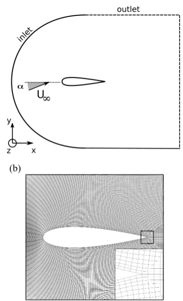
sur-Fig. 1 (a) Sketch of the computational domain. (b) Grid in the proximity of the aerofoil (nodes are plotted with a skip index of six). The inserted figure is an enlargement of the area surrounding the trailing edge.

face. By adjusting the value of the torsional stiffness, the flap movement can be selectively locked-in a specific flow frequency, thus introducing an additional dynamic mean of manipulating the flow . The paper is structured as follows. Initially in section (2) we will give a brief overview of the numerical methods and of the geomet-rical set-up that have been used. Then, in section (4) we will illustrate the results of the preliminary two-dimensional parametric campaign that we have carried out to roughly identify the quasioptimalconfiguration and location of the flaplet. Finally, in section (5) the results and the interpretation of the flow fields gener-ated by a full direct numerical simulations are offered also by comparing the characteristics of the fields ob-tained with and without flaplet. Some conclusions will be drawn at the end of the paper in section (6).

2 Baseline numerical formulation

To tackle the problem at hand, we consider an incom-pressible three-dimensional unsteady flow field, governed by the Navier-Stokes equations around a straight wing

with an infinite spanwise dimension. The computational domain is shown in figure (1a). The coordinate system is a Cartesian inertial one, with thex and y axis (x1

andx2) denoting the directions parallel and normal to

the aerofoil chord, andz (x3) being the axis normal to

the paper. Also,u,v andw(u1,u2 andu3) denote the

velocity components parallel and normal to the chord, and along the span respectively. With the given nota-tions, using Einstein’s summation convention, the di-mensionless equations that govern the incompressible flow motion are:

∂ui

∂t + ∂uiuj

∂xj

=−∂P

∂xi

+ 1

Rec

∂2ui

∂xj∂xj

+fi, (1)

∂ui

∂xi

= 0, (2)

The equations have been made non-dimensional using the magnitude of the free stream velocityU∞ and the

aerofoil chord c. Also, in the momentum equation (1),

Rec=U∞c/νis the Reynolds number andfirepresents a system of body forces used to keep into account the presence of the flap as it will be discussed later.

The momentum and mass conservation equations (1 and 2), are discretised on a cell-centered, co-located grid using a well-established curvilinear finite volume code [37, 36, 31, 32]. The fluxes are approximated by a second-order central formulation, and the method of Rhie and Chow [34] is used to avoid spurious pressure oscillations. The equations are advanced in time by a second-order semi-implicit fractional-step procedure [25], where the implicit Crank-Nicolson scheme is used for the wall nor-mal diffusive terms, and the explicit Adams-Bashforth scheme is employed for all the other terms. The pressure Poisson equation arising when imposing the solenoidal condition on the velocity field, is transformed into a series of two-dimensional Helmholtz equations in wave number space via Fast Fourier transform (FFT) in the spanwise direction. Each of the resultant elliptic 2D

problem is then solved using a preconditioned Krylov method (PETSc library [4]). In particular, the iterative Biconjugate Gradient Stabilized (BiCGStab) method preconditioned by an algebraic multigrid preconditioner (boomerAMG) [18] revealed to be quite efficient. The code is parallelized using a streamwise domain decom-position via the MPI message passing library. Further details on the code, its parallelisation and the exten-sive validation campaign that has been carried out in the past can be found in Rosti et al. [36].

ar-rangement (see figure (1b)). The grid is adapted to the three dimensional case by repeating the baseline 2D

grid uniformly in the spanwise direction. With this ar-rangement, the external surface that bounds the com-putational domain, contains both the inlet and the out-let (see figure (1a)). To determine which portions of the external bounding surface act as an inlet (or an outlet), at each time step a local spanwise average of the fluid velocity is evaluated in a tiny region close to the bound-ary. When the averaged flow direction points outward, the corresponding portion of the boundary is assumed to be an outlet, and is treated using a convective bound-ary condition. Conversely, if the mean flow direction is directed inward, the corresponding boundary surface is considered to be an inlet, and a Dirichlet type condition based on an irrotational approximation is used. In par-ticular, the values to be assigned to the velocity field on the Dirichlet portions of the boundary are determined by solving a companion potential equation discretised via the panel method of Hess and Smith [19].

The remaining boundary conditions are imposed as follows: impermeability and no slip conditions are set on the aerofoil wall, periodic conditions are assumed on the planes bounding the domain in the spanwise di-rection, and continuity of the flow variables is enforced through the top and bottom planes generated by the C-grid topology downstream of the trailing edge.

All the three-dimensional simulations that will be presented have been obtained at a chord Reynolds num-berRec = 20000. Differently, the two-dimensional para-metric study that will be presented in the next section has been carried out atRec = 2000. For both the 3D and the 2D simulations, the angle of attack has been set toα= 20o _{(stalled condition).}

The grid system that has been chosen for the three dimensional simulations, has been determined after a number of trial and errors tests and companion grid convergence studies. Finally, we have found that a grid composed by 2785×626×97 nodes (in thex1,x2andx3

directions, respectively), delivered a sound compromise between all the local resolution requirements set by the imposed high angle of attack: wing curvature, separa-tion, attached turbulent boundary layers and shear lay-ers embedded in the flow field. In terms of local wall units, in the attached turbulent layers, the correspond-ing mesh resolution verifies∆x+_<3.0,∆y+_{<0.5 and}

∆z+<7.5 (superscript + indicates standard local vis-cous units lengths: i.e., lengths made non dimensional using the kinematic viscosity ν, and the skin friction velocity uτ). Finally, the spanwise size of the domain has been set equal to 0.9c, which guarantees a good velocity decorrelation between the periodic end planes [36]. Further details on the procedure that has been

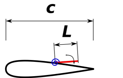
Fig. 2 Sketch of the flap hinged on the suction side of the aerofoil.

followed to generate the grid and the mesh refinement study campaign can be found in Rosti et al. [36].

2.1 Fluid-flap interaction model

Figure (2) shows the configuration that we have anal-ysed in this study, it comprises a NACA0020 aerofoil with a rigid, nominally infinitely thin flaplet of length

Lmounted on the wing suction side. The flap is hinged to the surface via a torsional spring that constraints its motion to take place on thex−y plane. The evolution of the flap angular displacement, θ(t) can be modeled using the canonical second order differential equation:

Iθ¨+Cθ˙+Kθ=T, (3)

In equation (3), I is the flap moment of inertia with respect to the rotation axis (i.e., I = mL2/3, m be-ing the mass of the flap per unit spanwise length), C

is an angular damping factor andKis the spring rota-tional stiffness (C andK are per unit spanwise length too). Finally, T is the total torque per unit spanwise length exerted by the fluid forces on the flap. When no damping is considered, a compact way to characterise the physical properties of the flap is based on specify-ing the sprspecify-ing stiffness K in terms of the moment of inertia I and its natural frequency f, obtained from the solution of the homogeneous equation associated to equation (3):K= (2πf)2I.

Estimate from the NS equations without

forcing term

Interpolate to

the Lagrangian grid Compute

Spread to the Eulerian grid

Solve the NS again considering the forcing term Integrate the force

along the flap to find the total torque Integrate the flap euation to find

the new angular position Update the position of the Lagrangian points and their velocity

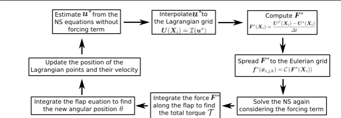
Fig. 3 Schematic of a full time step for the coupled fluid-wing-flap system.

at each time step, the integral of the elemental contri-butions of each force fi to the linear momentum bal-ance about the hinge provides the total torque forc-ing equation (3). The coupled algorithm that we have briefly described is based on a particular version of the immersed boundary (IB) method (i.e., the Reproducing Kernel Particle Method - RKPM method developed by Pinelli et al. [33]) that will be shortly revised hereafter.

In common with many others IB algorithms, the first stage of the algorithm involves a discretisation of the immersed body by distributing N nodes Xi,

i = 1, . . . , N (termed as Lagrangian points) over the surface bounding the immersed object. Generally, this set of nodes do not coincide with the underlying body fitted grid xi,j,k used to discretise the domain around the baseline aerofoil. This geometric discrepancy intro-duces the necessity of having a tool able to transfer the body forces defined on an immersed surface into equivalent forces defined over a local volume surround-ing the surface but belongsurround-ing to the body fitted grid. A discussion on the effect of spreading forces from the immersed surface into a volume comprising nodes of the C-grid used to mesh the aerofoil is posticipated at the end of this section. In the general framework of a pressure correction method, the second stage of the IB procedure involves a preliminary time advancement of the momentum equations without considering the pres-ence of the immersed surface. The obtained predicted velocity field u∗(xi,j,k) is then interpolated onto the embedded surfaceΓ:U(Xi) =I(u∗), where the veloc-ity corrections leading to the prescribed velocveloc-ity distri-bution on the surfaceUΓ _{are computed. These velocity} corrections, per time unit, can be interpreted as system of local body forces that restore the desired boundary conditions onΓ:

F∗(Xi) =U

Γ_(Xi)−U∗_(Xi)

∆t . (4)

In the final stage of the IB method, the previously ob-tained velocity fieldu∗_(x

i,j,k) is discarded and the mo-mentum equations are advanced again using the bound-ary restoring forces obtained in the predictive stage (4).

This force is evaluated on the fluid gridxi,j,k from the values atXi using a pseudo inverse of the operatorI, indicated withCand termed as spread. The spread op-eration formally allows to determine the singular forces on the fluid grid as:

f∗(xi,j,k) =C(F∗(Xi)). (5)

Aside from the flow field time advancement, also the position of the flap needs to be updated. Once the torque in equation (3) is computed by integrating each contribution of the singular forces F∗_(X

i) along the whole flap (equation (4)), the new angular positionθ(t) is found by integrating equation (3) in time. Finally, all the flap Lagrangian coordinates, and their respective velocities are updated consistently with a rigid body rotation about the hinge. The global time advancement scheme finalises with the solution of a pressure Poisson equation and the final projection of the velocity field onto the consistent divergence free space. A summary of the basic steps involved in the algorithm used to advance in time the fully coupled flap-fluid system is provided in figure (3).

The distinguishing feature of any continuous forcing IB method is related to the way in which the two op-eratorsI and Care applied. In our case, we follow the RKPM approach, used by Liu et al. [27], Liu et al. [28] and Zhang et al. [45], to construct a quasi Dirac’s delta function that can be defined on arbitrary supports [33]. The derived mollifier shares a number of momentum properties with a genuine delta function and therefore can be used to approximate both the interpolation and the spreading (i.e., convolution) operators as it would be formally done with a delta function in a distribution sense. As an example, the approximationfa(x) of the value of a given smooth function at point x ∈ Ω can be expressed as a convolution with a kernel functionwd having the first moments of a genuine Dirac’ s function as:

fa(x)≈

Z

Ω

Z

Ω

(x−s)i(y−t)j(z−v)kp(x−s, y−t, z−v)w(x−s, y−t, z−v)ds dt dv=

1 if i=j=k= 0

0 otherwise (7)

Because of the finite size of the support over which each regularised delta function acts to enforce the boundary conditions on the immersed object, the latter inherits an effective aerodynamic thickness. This thickness is re-lated to the actual size of the support that in turns is determined by the local mesh size (typically the effec-tive thickness is equivalent to the diagonal of a compu-tational cell). In summary, while the flow around the baseline aerofoil is simulated using a classical body fit-ted, C-grid, the effects on the flow generated by the flaplet and the dynamic of the latter are kept into ac-count via an immersed boundary method. In particular, the movement of the flap is determined via the integral of the fluid torques distributed along the flap itself. The local torques (per unit mass) are generated by the lo-cal accelerations computed by imposing the desired flap velocity at each time instant and the distance of each Lagrangian node to the flap hinge. The local accela-tion are obtained by interpolaaccela-tion from the body fitted grid into the immersed surface. On the other hand, the same singular force distribution is used as a set of body forces on the right hand side of the fluid momentum equations discretised on the body fitted grid. The op-eration to transform local forces distributed on a sur-face into a set of forces operating on a volume strip belonging to the body fitted mesh is carried out via a finite support compact pseudo Dirac’s delta function. As a consequence the actual shape of the flap is not seen as a sharp object by the fluid flow, but rather as a diffused volume strip with a finite (i.e. a non-zero) aerodynamic thickness (seen by the flow).Further de-tails on the RKPM IB method and its implementation in a finite volume context can be found in Pinelli et al. [33]. For an implementation in a Lattice Boltzmann framework including moving and deformable surfaces the reader can refer to Favier et al. [16].

3 Baseline flow characterisation

To introduce the main features of the flowfield that we wish to manipulate, we consider a NACA 0020 aerofoil at an angle of incidence of 20o _{and at chord Reynolds} number of 2×104. In these conditions the flow is mainly characterised by a large recirculation zone covering al-most the whole suction side as shown in figure (4a) [36]. Moreover, both a secondary counter rotating vortex lo-cated by the trailing edge, and another very small

re-Fig. 4 (a) Contours of mean flow streamwise velocity and streamlines. Contour goes from −0.3U∞ (blue) to 1.4U∞ (red). (b) Instantaneous liftcl(solid line) and dragcd(dashed

line) coefficients as a function of time.

Fig. 5 Contours of instantaneous flow streamwise veloc-ity and streamlines. Contour goes from −0.3U∞ (blue) to 1.4U∞(red), and the snapshots cover a full shedding period of 1.87c/U∞.

step (mean values: cl = 0.64 and cd = 0.35). From the figure, one can observe the presence of a dominant oscillation period clearly associated to the alternating vortex shedding in the wake, with a corresponding non dimensional frequency, in terms of Strouhal number, equal to St =fsc/U∞ ≈0.534 [36]. The unsteady

be-haviour of the spanwise vorticity field, determined by the shear layers instabilities and by the mutual inter-action of the vortices embedded in the wake, is the

ul-Fig. 6 Contours of the mean flowx-component velocityu. The colour contours are used for the 2Dcase, and goes from

−0.4U∞(blue) to 1.2U∞(red), while the contour lines (with the same levels separated by 0.6U∞) are used for the 3Dcase.

timate responsible of the aerodynamic response of the aerofoil to stalled conditions. For this reason, any con-trol strategy that aims at an overall improvement of the aerodynamic efficiency must tackle the direct manipu-lation of the vorticity field and its unsteadiness. Along this line of thought, this work investigates on the pos-sibility of controlling the vorticity field generated by an aerofoil at high angle of attack using a self adap-tive flaplet mounted on its suction side. In particular, the objective is to find a configuration that palliates the detrimental effects of stall by producing increased lift. To pursue such an objective, a parametric study covering a fully three-dimensional flow at the targeted chord Reynolds number would be computationally un-realistic. For this reason, a preliminary study on a low Reynolds number, fully laminar, two-dimensional flow has been carried out with the objective of bounding the parametric range that needs to be explored for achiev-ing a good flap design in a realistic three dimensional scenario. Before describing the initial two-dimensional parametric study, a comparison between the two base-line cases (i.e., fully 3D case at higher Reynolds number versus the laminar case at lower Reynolds numbers) will be introduced to provide a conceptual justifica-tion of the procedure that has been followed. Figure (6) compares the character of the mean three dimensional

x−wise velocity field at Rec = 2×104 and α = 20o with the two dimensional field obtained at the same angle of attack but at one order of magnitude smaller Reynolds number, i.e.,Rec = 2×103. The two velocity fields show similar qualitative features: large recirculat-ing regions of comparable magnitude coverrecirculat-ing the whole suction side of the aerofoil (i.e., the sizes of the recir-culating regions are 0.5c and 0.35c in the 2D and 3D

Case f /f0 L/c xF/c K×103 I×103 cl cd E

Ref − − − − − 0.93 0.50 1.86

F0.25-L0.10-X0.7 0.25 0.10 0.7 2.35 3.33 1.03 0.50 2.04 F0.50-L0.10-X0.7 0.50 0.10 0.7 9.38 3.33 0.90 0.49 1.84 F1.00-L0.10-X0.7 1.00 0.10 0.7 37.5 3.33 0.98 0.50 1.94 F2.00-L0.10-X0.7 2.00 0.10 0.7 150. 3.33 0.88 0.48 1.84 F4.00-L0.10-X0.7 4.00 0.10 0.7 600. 3.33 0.85 0.48 1.78 F0.25-L0.20-X0.7 0.25 0.20 0.7 9.38 13.3 0.93 0.51 1.84 F0.50-L0.20-X0.7 0.50 0.20 0.7 37.5 13.3 0.83 0.48 1.72 F1.00-L0.20-X0.7 1.00 0.20 0.7 150. 13.3 1.26 0.56 2.27 F2.00-L0.20-X0.7 2.00 0.20 0.7 600. 13.3 0.78 0.46 1.69 F4.00-L0.20-X0.7 4.00 0.20 0.7 2402 13.3 0.78 0.46 1.69 F0.25-L0.30-X0.7 0.25 0.30 0.7 21.1 30.0 0.71 0.45 1.55 F0.50-L0.30-X0.7 0.50 0.30 0.7 84.4 30.0 0.87 0.51 1.69 F1.00-L0.30-X0.7 1.00 0.30 0.7 337. 30.0 0.85 0.47 1.82 F2.00-L0.30-X0.7 2.00 0.30 0.7 1351 30.0 0.85 0.49 1.74 F4.00-L0.30-X0.7 4.00 0.30 0.7 5405 30.0 0.83 0.48 1.70 F1.00-L0.20-X0.6 1.00 0.20 0.6 150. 13.3 1.11 0.50 1.39 F1.00-L0.20-X0.8 1.00 0.20 0.8 150. 13.3 0.70 0.44 1.57

Table 1 Flap configurations considered in the 2D parametric study. Performance of each configuration is evaluated by the lift coefficientcl, the drag coefficientcd, and the efficiencyE=cl/cd. during a ramp-up manoeuvre. The aerofoil is NACA0020

and the Reynolds number isRec= 2000. The flap parameters, i.e., the ratio between the spring natural frequency and the

shedding frequency f /f0, the flap’s length L, the hinge positionxF, the spring rotational stiffness K, and the moment of

inertiaIis provided.

both the 2D and the 3D stalled cases is mainly deter-mined by the presence, the interaction and the shedding of the two large counter rotating vortices that charac-terise the region above the aerofoil (see figure (7)). The dynamic of these two large vortices governing the lift os-cillations, is mainly of 2D, laminar nature and basically involves only the interaction of the very large coherent structures embedded in the flow. Although the quanti-tative differences between the two-dimensional and the three-dimensional case are not negligible, the dominat-ing effects and the events sequencdominat-ing appear to be qual-itatively similar. Moreover, since the self adaptive flap that we will use extends over the whole span of the wing, no significant 3D effects will be introduced by its presence as the flaplet will mainly interfere with the largest integral scales of the flow which are intrinsically two-dimensional in character.

4 Flaplet design in 2D

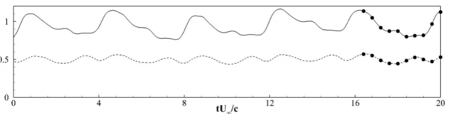
Motivated by the aforementioned considerations, we have initially focused on the geometrical properties (i.e., size and location) and the flap dynamic response (i.e., its natural frequency) that deliver anoptimalcondition in a two dimensional, fully laminar flow atα= 20o. Here, we define anoptimalcondition as the one that delivers the highest lift coefficient cl, preserving or improving the aerodynamic efficiencyE=cl/cd. We have started our analysis by considering the low Reynolds number (i.e.,Rec= 2×103), 2Dflow over a NACA0020 aerofoil at α= 20o without any added flap. Figure (8) shows

the time evolution of the lift and drag coefficients for the baseline configuration. Both coefficients are char-acterised by periodic oscillations: every period of lift coefficient corresponds to the shedding of a vortex, at a shedding frequency equal tofs= 0.555U∞/c. The lift

coefficient evolution also shows the presence of a lower frequency f = 0.308U∞/c (almost half the shedding

Fig. 7 Contours of the instantaneous spanwise component of vorticityωz, corresponding to the minima (a,b) and

max-ima (c,d) locations of the lift coefficient over one shedding period for the 2D (a,c) and 3D (b,d) cases. Blue lines used for negative, clockwise vorticity, red ones for positive values (±5U∞/c).

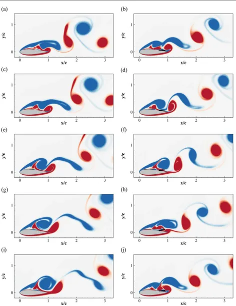
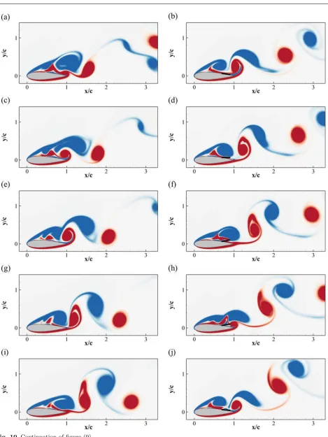
in lift, and with an impact in determining the structure of the near-wake (see figure (9i) and figure (10i)). The final snapshots of the series, correspond to the end of the cycle with the generation of a new lifting vortex leading to the beginning of a new cycle.

Next, we have proceeded to perform a parametric study on the aerodynamic effects of the flaplet configu-ration. In particular, the flap reaction to the underlying

unsteady flow field can be tuned by acting on various parameters: its length, position, inertia, spring stiffness and damping factor. The outcomes of the analysis con-ducted by varying the aforementioned parameters are summarised in table (1) reporting some typical vari-ations of the averaged aerodynamic coefficients (last three columns) when changing the flaplet characteris-tics (second to fifth columns). In particular, the length

Lof the flap was varied between 0.1c and 0.3c, the po-sition of the flap hingexF ranged between 0.6cand 0.8c (measured from the leading edge), the stiffnessKof the spring was set such that its natural frequencyf was be-tween 1/4th and 4 times the shedding frequencyf0 of

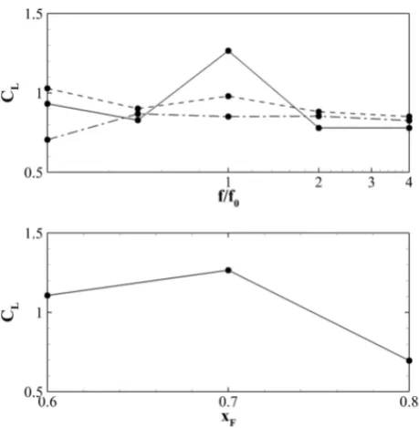
the baseline case without flap. The effects of the length and stiffness of the torsional spring on the value of the mean lift coefficientcl are also reported graphically in figure (12a). Anoptimumcondition (i.e., maximum lift increase with respect to the baseline case) is achieved with a flaplet 0.2c long, resonating with the shedding frequency (flap natural frequency equal to the shed-ding one). Except for the cases of flaplets of very low natural frequency, if the latter doesn’t match the base-line flow shedding frequency, the lift coefficient turns out to be almost unaffected by the length of the flap. On the other hand, when considering resonating con-ditions, the maximum lift and efficiency are achieved using a flaplet L = 0.2c long, a size roughly corsponding to half the dimensions of the recirculation re-gion. Figure (12b) shows how the lift coefficient changes as a function of the hinge position when considering a

L= 0.2clong flaplet in resonating conditions. The opti-malposition, in terms of maximum lift, is at about 0.7c, where, when unlifted, the flaplet end almost reaches the trailing edge.

In summary, when a low Reynolds number, 2Dcase at an angle of attack ofα= 20o_{is considered, the flaplet} configuration that maximises the mean lift features a length of 0.2c, a hinge location at 0.7c and a spring stiffness leading to a flaplet natural frequency match-ing the sheddmatch-ing one. For this specific flow condition and with the mentioned configuration, the flaplet inter-feres actively with the unsteady vorticity field delivering a 20% increase in the average aerodynamic efficiency. The corresponding time variations of the liftcland drag

cd coefficients are reported in figure (11) together with the elevationy of the tip of the flap from the surface of aerofoil. The time averagedcl is 35% higher than the case without flap (see figure (8)), while the shedding frequency remains unchanged (i.e., fs = 0.555U∞/c).

Fig. 8 Instantaneous lift cl (solid line) and drag cd (dashed line) coefficients as a function of time. The dots indicate the

selected time snapshots shown in figure (9) and figure (10).

attaining almost the same value at each shedding pe-riod (see figure (8)). The right columns in figure (9) and figure (10) show the spanwise vorticity over two shedding cycles at the times marked in figure (11a). In the initial snapshots (figure (9b, d)), when the flap is almost laying on the aerofoil surface, a first vortex de-taches from the trailing edge. Next, (figure (9f, h)) the flap reaches its maximum elevation while a large lifting vortex is formed above the aerofoil inducing a maxi-mum lift force. The cycle is closed by the formation of a new trailing edge vortex (figure (9j) and figure (10b)). The mutual interaction of the flow field with the flaplet has a strong impact on the shedding process and there-fore on the structure of the wake (see figure (10b) and figure (10j)). The importance of the interaction is fur-ther stressed by the high correlation between the lift oscillations and the flap motion (correlation coefficient is ≈0.6), and in particular by the fact that the mum lift is reached when the flap is almost at its maxi-mum elevation (the time lag between the two functions is≈0.2c/U∞).

As a further measure of the effect of the flaplet on the vorticity field, we have quantified the circula-tions of the velocity field along two closed rectangular loops bounding the lifting vortex (x ∈ [0.5,1.0], y ∈

[0.3,0.6]), and the trailing edge vortex (x ∈ [0.8,1.3],

y∈[0.0,0.3]), respectively (see figure (7)). The circula-tion of the leading edge vortex which is responsible for the lift generation is only slightly increased by the pres-ence of the flaplet (i.e.,≈3%), while the circulation of the trailing edge vortex, responsible for the generation of the downforce, is substantially reduced by a factor of ≈ 20%. Therefore, the increase in the average lift induced by the presence of the flaplet is mainly related with i) the regularisation of the shedding process and with ii) the reduction of the downward force induced by the trailing edge vortex.

This preliminary study conducted in a simplified 2D, laminar scenario has allowed to determine a point

in the parameters space leading to a maximum increase in both lift and aerodynamic efficiency. The analysis has also characterised the features of the unsteady vortic-ity fields that develops when the optimal flap is used. The validity of our conjecture about the possibility of extending the results obtained with a simplified 2D sce-nario to a realistic 3D one will be discussed next.

5 Effect of the adaptive flaplet on a 3D aerofoil

We now compare the three-dimensional flow fields around

a NACA0020 at an angle of incidence of 20o _{and at}

Rec= 2×104, obtained when considering the unmodi-fied aerofoil and when equipping the wing with a flaplet extending along its whole span, and featuring the quasi

optimalconfiguration discussed in the previous section (flap length L = 0.2c, hinge location at x = 0.7c). Furthermore, inspired by the two-dimensional results, the stiffness of the torsional spring has been set to

K= 0.150 leading to a natural frequency that matches the shedding one of the unmodified aerofoil.

Fig. 9 Contours of the instantaneous spanwise component of vorticity ωz during two shedding cycles (corresponding to

Fig. 11 Optimal flaplet configuration: instantaneous liftcl (solid line) and dragcd(dashed line) coefficients as a function of

time. The thin solid line represents the elevationyof the tip of the flap. The set of bullets on the graphs indicates the instants in time where the vorticity snapshots have been sampled, see figure (9) and figure (10).

Fig. 12 Mean lift cl as a function of (a) the spring natural

frequency f and of (b) the position of the hinge xF. The

dashed, solid and dash-dot lines are used for the cases with L= 0.1c,L= 0.2candL= 0.3c, respectively.

modify the value of the associated Strouhal number

St=fsc/U∞that remains fixed toSt= 0.534, a value that is almost the same as the one found in the 2D case at lower Reynolds number.

When we compare the mean pressure coefficients

Cp of the two configuration, as shown in figure (14a), we notice that the pressure on the suction side of the aerofoil with flap is reduced upstream the flap posi-tion, thus generating a higher lift, in agreement with the results by Schatz et al. [38] and Bramesfeld and Maughmer [8], and then increases, downstream the lo-cation of its hinge. The friction coefficientCf, reported in figure (14b), shows that the two aerofoils have a simi-lar friction profile, with an early leading edge separation

Fig. 13 (a) Liftcl(black) and dragcd(gray) coefficients as a

function of time. (b) Evolution of the aerodynamic efficiency E=cl/cd. Solid lines are used for the aerofoil with flap, while

dashed lines for the reference values.

located atx≈0.025c [36], except, in the leading edge peak which is enhanced by 10% in the case with flap.

Fig. 14 (a) PressureCP and (b) frictionCf coefficient

dis-tributions. Solid and dashed lines are used for the aerofoil with and without flap, respectively.

Fig. 15 Contours of the mean (i.e., time and z-averaged) spanwise component of vorticityωz and mean streamlines of

the NACA 0020 aerofoil atα= 20o _andRe

c= 2×104. Left

panel (a): results for the baseline wing; right panel (b): wing equipped with a flaplet (L = 0.2c,xF = 0.7c,K = 0.150).

Blue negative vorticity (clockwise), red positive (±7U∞/c).

Fig. 16 Meanx-wise (a) andy-wise (b) velocity components profiles over the aerofoil and in the near wake. Lines are used for the aerofoil without flap; symbols refer to aerofoil with flap.

reduces the size of the positive vorticity recirculating region by the trailing edge, also displacing the peak of positive vorticity further downstream, well beyond the trailing edge.

More information on the mean flow can be educed from the velocity profiles in figure (16) where thexand

y velocity components are shown. While the mean flow velocity on the pressure side is basically unaffected by the presence of the flaplet, on the suction side the ve-locity field changes in the region spanned by the flap movement. As compared to the baseline case, upstream of the flap location, atx= 0.6c, both velocity compo-nents are reduced in amplitude, with a corresponding overall reduction of reversed flow. Downstream of the flap, at x = 0.9c, in the region traversed by the flap oscillations, the velocity intensity is reduced because of the no-slip and no-penetration boundary condition on the flap solid surface. Finally, in the near wake region, the velocity defect is slightly enhanced in the case with flap.

The effects of the flaplet on the flow become more visible when considering the distribution of higher order statistical quantities. Figure (17a), shows a comparison of the averaged turbulent kinetic energy k = 1/2 < u0_iu0_i>, in the controlled and uncontrolled cases. Consis-tently with the upstream laminar conditions, the kinetic energy is initially zero for both the aerofoils. Further downstream in the shear layer originated at the lead-ing edge, k starts to grow similarly in both cases. On the other hand, the second shear layer formed past the trailing edge is influenced by the action of the flaplet. Its motion reduces the intensity of the velocity fluctua-tions. Downstream of the aerofoil, the two shear layers merge into the wake where the reduced levels ofk, due to the flaplet action, are evident. This is clearly visible from figure (17b) showing the turbulent kinetic energy profile atx≈5.5c.

As previously mentioned, one of the consequences of the action of the flaplet on the flow field is the re-duction in the intensity of the backflow on the aerofoil surface. To quantify this effect, in figure (18) we display the probability of finding a negative streamwise veloc-ity componentP(u <0) in the two cases. In both situa-tions, this probability is obviously zero in the outer flow where the uvelocity is always positive, while its value increases in the recirculating region. In the reference case, the highest probability of backflow corresponds to the region close to the trailing edge, atx≈0.8. In the case where the flaplet is active, the probability of having backflow is remarkably reduced not only in the region spanned by the flap movement but also upstream of it. To gain further insight on the effect of the flaplet-flow interaction we have used the classical Q-criterion

Fig. 18 Intermittency factor I− = P(u <0) for the ref-erence (a) and flap (b) cases. Contour levels go from blue (I−= 0) to red (I−= 1).

Fig. 19 Visualisation of instantaneous vorticity field by means of Q-iso-surfaces (Q = 450U2

Fig. 20 Visualisation of instantaneous vorticity field by means ofQ-iso-surfaces (Q= 450U2

∞/c2) coloured by the spanwise vorticity. (a) and (b) are the cases without and with the flap, respectively.

proposed by Hunt et al. [21]. This technique assigns a vortex to all spatial regions that verify the condition

Q=1 2 |Ω|

2_{− |S|}2

>0, (8)

where S = 1₂ ∇u+∇uT is the strain rate tensor

and Ω = 1

2 ∇u−∇u

T

is the vorticity tensor. In-stantaneous Q iso-surfaces corresponding to the case without and with flaplet are shown in figure (19) and figure (20). From the first figure, it appears that the action of the flap contributes to the reductions of both the backflow and the generation of turbulent structures upstream of its location. Moreover, coherent structures in the wake dissipate faster in presence of the flaplet consistently with the drop observed in the profiles of turbulent kinetic energy (figure (17)). From the second figure, it is possible to recognise the principal flow fea-tures of the baseline case [36]. These are summarised hereafter to introduce the comparison with the flaplet case. Initially, the incoming laminar flow separates at the leading edge, forming a shear layer that rolls up into Kelvin-Helmholtz (KH) vortices [12, 13, 44, 41, 1]; this instability, locally, triggers the flow transition to turbu-lence; further downstream, the turbulent separated re-gion appears to be characterized by fine texture, small-scale eddies, eventually merging into coherent larger structures; finally behind the aerofoil, a large turbu-lent wake is formed, the dynamics of which are similar to a von Karman vortex street typical of bluff body wakes. In contrast to classical vortex shedding process showing an alternately series of vortices of opposite sign and equal strength, here the wake is highly asymmet-ric presenting vortices of uneven strength. The loss of symmetry and the irregularity of the vortices pattern is

related to the interaction between the two vortex gen-erating mechanisms [10, 9]: the vortices rolling up under the action of the KH leading edge shear layer instabil-ity and the street of vortices shedding from the trailing edge. The main features of this flow process, largely present also in the 2D, laminar case, remain practically unaffected by the presence of the flap, except in the leading edge area, where the KH instability is delayed further downstream (figure (20)). The regularisation of the shedding of vortices from the leading edge is respon-sible of the increased pressure coefficient (figure (14a)), that ultimately produce the increased lift coefficient.

To study the differences in the shear-layer char-acteristics between the baseline case and the optimal flap simulation, we carried out a Finite Time Lyapunov Exponent (FTLE) analysis. This technique is a La-grangian coherent structures educing technique, see Haller [17] and Shadden et al. [40], that highlights the presence of strong shear layers in separated flows. The FTLE

σT_{(x, t) is a scalar function of space and time which} measures the rate of separation of neighbouring parti-cle trajectories initialised within a small ball centred at xat timet, and is defined as

σT(x, t) = 1

Tln

p

λmax(∆). (9)

Here,λmax(∆) is the largest singular value of the Cauchy-Green deformation tensor computed over a finite time interval [t0, t0+T]

∆= ∂x(t0+T,x0, t0)

∂x0

. (10)

Fig. 21 Istantaneous contour plot of the FTLEσT _{during a shedding period for the case with flap. The contour levels go}

from 0 (white) to 7U∞/c(red). The black contour lines are used for the baseline case without flap.

while at the leading edge shear layer rolls up under the action of a KH instability. Figure (21b-d) show how the trailing edge shear layer undergoes a KH instability and a vortex is generated. The detachment of the vor-tex is illustrated in figure (21e-f). In the two cases, the instantaneous shapes of the leading edge shear layers are very similar. However, the locations of the trailing edge vortex cores at these two time instants (panels b and d of figure (21)) do not correspond with the con-trolled case showing a streamwise shift of the actual position. This relative displacement is induced by the downward movement of the flap and the consequent ap-peareance of a positive streamwise velocity generated by the relative movement of the flap and the aerofoil which will be analysed later on. The opposite effect is also visible during the flap lifting phase (panels c and d), when fluid momentum is entrained upstream by the flap movement.

By looking at the time variation of the vorticity field another important effect of the interaction

figure (23a)). The presence of the flaplet alters the pre-viously described sequence. Here, the initial snapshot has been chosen to match the condition in which the flaplet lays on the aerofoil surface (figure (22b)). In this situation, the trailing edge vortex has just been shed, and the lifting vortex is forming. As the flap lifts up (figure (23d, f)) under the action of the pressure gra-dient induced by the passage of the lift vortex, a new trailing edge vortex is formed while the lifting vortex is shed away. As a consequence, the flap moves downward (figure (23f, h, j)) under the action of the trailing edge vortex that is forming and subsequently, detaches from the trailing edge. The formation and roll up of the trail-ing edge vortex is conditioned by the movement of the flap that during its downward rotation generates a jet that pushes the vortex downstream. The displacement of the trailing edge vortex away from the aerofoil at every shedding cycle allows the incoming lifting vortex to grow and develop more freely without the constraint generated by the vicinity of a counter rotating vortex. The detachment of the trailing edge vortex induced by the flap generated jet has also a regularisation effect on the shedding cycle that now repeats identically with no difference between consecutive cycles. As the snapshots indicate, the position of the flap is strongly related with the passage of the lifting vortex. In particular, we have measured a correlation coefficient between the evolu-tion of the lift and the flap posievolu-tion equal to 0.6. These findings are quite similar to the ones observed for the 2D laminar flow where the flaplet was regularising the lift/drag cycle with a movement characterised by the same value of the lift-flap position correlation coeffi-cient.

To shed some more light on the mechanism driv-ing the flap motion and the corresponddriv-ing lift increase, in figure (24) we consider the instantaneous streamwise velocity profiles (displayed in the top panel) and the pressure coefficients (shown in the bottom one), sam-pled at two time instants corresponding to an ascend-ing and descendascend-ing flap movement. Note that all the profiles have been obtained after having averaged in the spanwise, homogeneous direction. When the flap is moving downward (blue line), the large recirculation re-gion (negative velocity) is enclosed between the outer flow at the top, and a region characterised by positive velocities at the bottom. The fluid trapped in this re-gion is displaced downstream under the action of the low pressure values associated with the core of the trail-ing edge vortex. This observation is confirmed by the pressure coefficient recorded at the same time instant showing a strong negative value at the trailing edge consistently with the incipient formation of the trail-ing edge vortex (see figure (23h)) and a decrease of the

Fig. 24 (Top) Spanwise averaged streamwise velocity pro-fileuas a function of they-coordinate at two time instants. Three velocity profiles are provided: atx= 0.85c, 0.9cand 0.95c. Note that, the profiles have been shifted for clarity in-dicating with the vertical dashed line the respectives zeros. (Bottom) Spanwise averaged pressure coefficientCprecorded at the same time instants as above. In particular, in both pan-els, the blue and red lines correspond to the downward and upwards rotation of the flap, figure (23h) and figure (23d), respectively.

torque T acting on the flap. On the other hand, dur-ing the upward motion of the flap (red line) the sign of the recorded streamwise velocity in the region between the flap and aerofoil is negative. In this condition, the full detachment of the trailing edge vortex figure (23d) reduces the suction also allowing for an increase of the torque on the flap.

To provide a phenomenological explanation on the

Fig. 25 Contours of the conditional averaged spanwise com-ponent of vorticityωz, for the case with (b, d) and without

(a, c) flap. Blue negative vorticity (i.e., clockwise), red posi-tive (±5U∞/c). The top and bottom rows correspond to the times of maximum and minimum lift, respectively.

shows an almost uniform sequencing of the counter ro-tating vortices sharing the same spatial locations. The enhanced regularity of the cycle is also confirmed in figure (26a) showing the time cross correlationρof the lift coefficient cl and the spanwise vorticityωz at loca-tion (2.0c; 0.4c) (xcoordinate measured from the lead-ing edge,yfrom the profile chord). The cross correlation

ρis defined as follows

ρ(τ) = E[cl(t)ωz(t+τ)]

σ[cl] σ[ωz]

, (11)

where E[ ] and σ[ ] indicate the expected value and the standard deviation, respectively. In the case with flap, the evolution of the time cross correlation shows a clear periodic behaviour with high levels of correlations (0.35). While in the case without flap, the correlation is much lower (0.05). Finally, the right panel of the figure shows the time cross correlations of the lift and drag coefficients with the flap movement defined by its ele-vation y. As already said, both the aerodynamic force coefficients are strongly correlated with the flap move-ment, especially the lift coefficient which has a value of cross correlation almost double the one for the drag efficient. A phase shift is also apparent for the drag co-efficient, whose peaks slightly precede the one of the lift coefficient. To summarise the last results, all this cross-correlation graphs show that the aerodynamic coeffi-cients are strongly linked with the flap movement and with the vorticity field, proving that the flap movement is determined and linked with the vortex dynamic which ultimately determines the aerodynamic behaviour.

As already done in the 2Dcase, to determine which mechanism is the main responsible for the increase in average lift obtained with the flap, we have computed the circulation Γ over two closed surfaces C embed-ding the lift and the trailing edge vortices, respectively. The former is defined over the region x ∈ [0.5,1.0],

y ∈ [0.3,0.6], the latter covers the area x∈ [0.8,1.3],

y∈[0.0,0.3] (see figure (7)). Similarly to what we have observed for the 2Dlaminar case, the circulation of the leading edge vortex (the one that generates lift) is only slightly increased by the flap presence (≈ 2%), while the circulation of the trailing edge vortex (the one that reduces the lift, or increase the downforce) is substan-tially reduced by a factor of≈15%.

6 Conclusion

Fig. 26 (a) Time cross correlationρof the lift coefficientcland spanwise vorticityωzat the location (2.0c; 0.4c). Solid and

dashed lines are used for the case with and without flap, respectively. (b) Time cross correlation ρof the lift coefficient cl

(solid line) and drag coefficientcd(dashed line) with the flap elevation.

the characteristics (i.e., size, location and natural fre-quency) of a self-adaptive flaplet able to deliver sub-stantial aerodynamic benefits in an otherwise stalled condition. This initial study has been conducted on a baseline NACA0020 aerofoil at 20o _{degrees angle of} at-tack at low (fully laminar) chord Reynolds number (i.e.,

Rec = 2×103). The impact on the aerodynamic per-formance of a rigid, thin flap hinged with a torsional spring on the aerofoil suction side has been analysed via a parametric study involving the size of the flap, the hinge location and the spring stiffness. It has been found that it is of fundamental importance to lock-in the flap oscillation frequency with the foil Strouhal number. In resonating conditions, the lift response be-come quite sensitive to the geometric properties of the flap. In particular, the quasioptimalperformances (i.e.,

≈20% increase in lift) are achieved with a flap length of one fifth of the chord hinged at about 70% of the aerofoil. Having determined the geometric and physi-cal character of an aerodynamiphysi-cally efficient flaplet, we turned our attention to the understanding of the mech-anisms responsible for the improved foil performances at high angle of attack. To this end, we have carried out Direct Numerical Simulations of the flow past a NACA0020 aerofoil at 20o angle of attack at a chord Reynolds number of 2×104 _{considering both the}

base-line wing and the wing equipped with the quasioptimal

flaplet determined in the 2Dparametric campaign. Ini-tially, considering the baseline wing, we have confirmed that the flow mechanisms taking place in the fully three-dimensional scenario, involving a laminar separation, a subsequent reattachment and a laminar-turbulent tran-sition, determine a flow behaviour that is qualitatively similar to the two dimensional case used for the pre-liminary design study. The reasons for this similarity are related with the common laminar separation, and the convective inviscid instability of the leading edge shear layer responsible for the roll up of the large recir-culation bubble on the aerofoil. In a second phase, we

have systematically compared the flow fields generated with and without the flap. Although the mean velocity fields and the mean kinetic energy are very similar, the flaplet has a very strong impact in manipulating the unsteady character of the vorticity field. In particular, the flap is popped up by the passage of the lift vortex and when relaxing back to the equilibrium position gen-erates a jet almost tangent to the wing surface, directed towards the trailing edge. This jet detaches the vortex street generated by the trailing edge shear layer insta-bility away from the aerofoil. The displacement of the trailing edge vortices has a twofold effect. On one hand there is a net decrease in the downforce that is directly generated by these vortices leading to a global increase of the lift. On the other hand, the displacement of the trailing edge vortex allow for a complete evolution of the leading edge generated vortex that now does not interact directly with the trailing edge vortices. As a consequence, the periodic character of the wake is now mainly controlled by the shedding of the leading edge vorticity into the wake that regularises the shedding cy-cle also promoting a much more ordered wake topology.

Compliance with Ethical Standards

Funding: this study was funded by the European Com-mission, 7th framework projectPelskin(grant number 334954) and by the EPSRC, projectQuiet Aerofoils of the Next Generation(grant number EP/N020413).

Conflict of Interest: the authors declare that they have no conflict of interest.

References

2. M A Aldheeb, W Asrar, E Sulaeman, and A A Omar. A review on aerodynamics of non-flapping bird wings. Jour-nal of Aerospace Technology and Management, 8(1):7– 17, 2016.

3. A Altman and G Allemand. Post-stall performance im-provement through bio-inspired passive covert feathers. In 54th AIAA Aerospace Sciences Meeting, page 2042, 2016.

4. S Balay, S Abhyankar, M Adams, J Brown, P Brune, K Buschelman, L Dalcin, V Eijkhout, W Gropp, D Kaushik, M Knepley, L C McInnes, K Rupp, B Smith, S Zampini, and H Zhang. PETSc Web page, 2015. 5. D W Bechert, M Bruse, W Hage, and R Meyer.

Biologi-cal surfaces and their technologiBiologi-cal applicationlaboratory and flight experiments on drag reduction and separation control.AIAA paper, 1960, 1997.

6. D W Bechert, W Hage, and R Meyer. Self-actuating flaps on bird-and aircraft-wings. Flow phenomena in nature: inspiration, learning and applications 2 (design and na-ture), pages 435–446, 2006.

7. DW Bechert, M Bruse, W Hage, and R Meyer. Fluid mechanics of biological surfaces and their technological application. Naturwissenschaften, 87(4):157–171, 2000. 8. G Bramesfeld and M D Maughmer. Experimental

investigation of self-actuating, upper-surface, high-lift-enhancing effectors. Journal of aircraft, 39(1):120–124, 2002.

9. M Breuer and N Jovicic. An les investigation of the sepa-rated flow past an airfoil at high angle of attack. InDirect and Large-Eddy Simulation IV, pages 165–172. Springer, 2001.

10. M Breuer and N Jovicic. Separated flow around a flat plate at high incidence: an les investigation. J. Turbul, 2(1):N18, 2001.

11. C Br¨ucker and C Weidner. Influence of self-adaptive hairy flaps on the stall delay of an airfoil in ramp-up motion. Journal of Fluids and Structures, 47:31–40, 2014. 12. S Burgmann, J Dannemann, and W Schr¨oder.

Time-resolved and volumetric piv measurements of a transi-tional separation bubble on an sd7003 airfoil. Experi-ments in Fluids, 44(4):609–622, 2008.

13. S Burgmann and W Schr¨oder. Investigation of the vortex induced unsteadiness of a separation bubble via time-resolved and scanning piv measurements. Experiments in fluids, 45(4):675–691, 2008.

14. A C Carruthers, A L R Thomas, and G K Taylor. Au-tomatic aeroelastic devices in the wings of a steppe ea-gle aquila nipalensis. Journal of Experimental Biology, 210(23):4136–4149, 2007.

15. H Choi, H Park, W Sagong, and S Lee. Biomimetic flow control based on morphological features of living crea-turesa).Physics of Fluids (1994-present), 24(12):121302, 2012.

16. J Favier, A Revell, and A Pinelli. A lattice boltzmann– immersed boundary method to simulate the fluid inter-action with moving and slender flexible objects. Journal of Computational Physics, 261:145–161, 2014.

17. G Haller. Distinguished material surfaces and coherent structures in three-dimensional fluid flows. Physica D: Nonlinear Phenomena, 149(4):248–277, 2001.

18. V E Henson and U M Yang. Boomeramg: a parallel al-gebraic multigrid solver and preconditioner.Applied Nu-merical Mathematics, 41(1):155–177, 2002.

19. J L Hess and A M O Smith. Calculation of potential flow about arbitrary bodies. Progress in Aerospace Sciences, 8:1–138, 1967.

20. W X Huang, S J Shin, and H J Sung. Simulation of flexible filaments in a uniform flow by the immersed boundary method. Journal of Computational Physics, 226(2):2206–2228, 2007.

21. J C R Hunt, A A Wray, and P Moin. Eddies, stream, and convergence zones in turbulent flows. Center for turbu-lence research report CTR-S88, pages 193–208, 1988. 22. J Johnston and A Gopalarathnam. Investigation of a

bio-inspired lift-enhancing effector on a 2d airfoil. Bioin-spiration & biomimetics, 7(3):036003, 2012.

23. J M Johnston, A Gopalarathnam, and J Edward. Exper-imental investigation of bio-inspired high lift effectors on a 2-D airfoil. North Carolina State University, 2011. 24. K H Kernstine, C J Moore, A Cutler, and R Mittal.

Ini-tial characterization of self-activated movable flaps,pop-up feathers. AIAA paper, 369, 2008.

25. J Kim and P Moin. Application of a fractional-step method to incompressible navier-stokes equations. Jour-nal of computatioJour-nal physics, 59(2):308–323, 1985. 26. T Liu, J Montefort, and S Pantula. Effects of flexible fin

on low-frequency oscillation in post-stalled flows. AIAA Journal, 48(6):1235–1247, 2010.

27. W K Liu, Y Chen, R A Uras, and C T Chang. General-ized multiple scale reproducing kernel particle methods. Computer Methods in Applied Mechanics and Engineer-ing, 139(1):91–157, 1996.

28. W K Liu, S Jun, and Y F Zhang. Reproducing kernel particle methods. International journal for numerical methods in fluids, 20(8-9):1081–1106, 1995.

29. R Mittal and G Iaccarino. Immersed boundary methods. Annual Review of Fluid Mechanics, 37:239–261, 2005. 30. J Montefort, N Pohl, T Liu, J Gregory, and J Crafton.

Thin-wing vibration control using flexible fins. AIAA journal, 51(9):2218–2230, 2013.

31. M Omidyeganeh and U Piomelli. Large-eddy simulation of three-dimensional dunes in a steady, unidirectional flow. part 1. turbulence statistics. Journal of Fluid Me-chanics, 721:454–483, 2013.

32. M Omidyeganeh and U Piomelli. Large-eddy simulation of three-dimensional dunes in a steady, unidirectional flow. part 2. flow structures.Journal of Fluid Mechanics, 734:509–534, 2013.

33. A Pinelli, I Z Naqavi, U Piomelli, and J Favier. Immersed-boundary methods for general finite-difference and finite-volume navier–stokes solvers.Journal of Com-putational Physics, 229(24):9073–9091, 2010.

34. C M Rhie and W L Chow. Numerical study of the tur-bulent flow past an airfoil with trailing edge separation. AIAA journal, 21(11):1525–1532, 1983.

35. M E Rosti, L Kamps, C Bruecker, M Omidyeganeh, and A Pinelli. The PELskin project-part V: towards the con-trol of the flow around aerofoils at high angle of attack using a self-activated deployable flap. Meccanica, pages 1–14, 2016.

36. M E Rosti, M Omidyeganeh, and A Pinelli. Direct numer-ical simulation of the flow around an aerofoil in ramp-up motion.Physics of Fluids, 28(2), 2016.

37. M E Rosti, M Omidyeganeh, and A Pinelli. Passive con-trol of the flow around unsteady aerofoils using a self-activated deployable flap. Journal of Turbulence, pages 1–25, 2017.

38. M Schatz, T Knacke, F Thiele, R Meyer, W Hage, and D W Bechert. Separation control by self-activated mov-able flaps. AIAA Paper, 1243:2004, 2004.

40. S C Shadden, F Lekien, and J E Marsden. Definition and properties of lagrangian coherent structures from finite-time lyapunov exponents in two-dimensional aperiodic flows. Physica D: Nonlinear Phenomena, 212(3):271– 304, 2005.

41. P R Spalart and M K Strelets. Mechanisms of transition and heat transfer in a separation bubble.Journal of Fluid Mechanics, 403:329–349, 2000.

42. L W Traub and L Jaybush. Experimental investigation of separation control using upper-surface spoilers. Journal of Aircraft, 47(2):714–718, 2010.

43. C H John Wang and J Schluter. Stall control with feath-ers: Self-activated flaps on finite wings at low reynolds numbers. Comptes Rendus M´ecanique, 340(1):57–66, 2012.

44. Z Yang and P R Voke. Large-eddy simulation of boundary-layer separation and transition at a change of surface curvature.Journal of Fluid Mechanics, 439:305– 333, 2001.