Condition-based maintenance of naval propulsion systems : data analysis with minimal feedback

Condition-Based Maintenance

of Naval Propulsion Systems:

Data Analysis with Minimal Feedback.

Francesca Cipollinia, Luca Onetoa, Andrea Coraddub,∗, Alan John Murphyc, Davide Anguitaa

a

DIBRIS - University of Genova, Via Opera Pia 13, I-16145 Genova, Italy

b

Naval Architecture, Ocean & Marine Engineering Strathclyde University, Glasgow G1 1XW, UK

c

Marine, Offshore and Subsea Technology Group, School of Engineering Newcastle University, Newcastle upon Tyne, NE1 7RU, UK

Abstract

The maintenance of the several components of a Ship Propulsion Systems is an onerous activity, which need to be efficiently programmed by a ship-building company in order to save time and money. The replacement policies of these components can be planned in a Condition-Based fashion, by pre-dicting their decay state and thus proceed to substitution only when really needed. In this paper, authors propose several Data Analysis supervised and unsupervised techniques for the Condition-Based Maintenance of a ves-sel, characterised by a combined diesel-electric and gas propulsion plant. In particular, this analysis considers a scenario where the collection of vast amounts of labelled data containing the decay state of the components is unfeasible. In fact, the collection of labelled data requires a drydocking of the ship and the intervention of expert operators, which is usually an in-frequent event. As a result, authors focus on methods which could allow only a minimal feedback from naval specialists, thus simplifying the dataset collection phase. Confidentiality constraints with the Navy require authors to use a real-data validated simulator and the dataset has been published for free use through the OpenML repository.

∗

Corresponding Author

Email addresses: [email protected](Francesca Cipollini), [email protected](Luca Oneto), [email protected] (Andrea Coraddu),[email protected](Alan John Murphy),

Keywords: Data Analysis, Naval Propulsion Systems, Condition-Based Maintenance, Supervised Learning, Unsupervised Learning, Novelty Detection, Minimal Feedback.

1. Introduction

Maintenance is one of the most critical tasks to be designed and pro-grammed by any product-selling company [1, 2, 3, 4]. As a fact, every complex system is designed assigning it a specific life-cycle, which is influ-enced by different factors such as the raw materials adopted, the estimated working hours, and the environmental conditions [5, 6]. Nevertheless, this time-to-live information is inevitably inaccurate as it is impossible to pre-dict at design phase the exact working conditions in which the system will operate [7, 8]. In any case, the decay of the system components will require at some point of time to be repaired or replaced, thus leading to the sys-tem halt to perform some maintenance tasks [9]. This is the reason why an efficient maintenance program can be time and costs saving since replac-ing a malfunctionreplac-ing component after it has failed durreplac-ing service, results in multiple downsides for the system owner company.

The Shipbuilding industry is particularly affected by this problem, as a ship breakdown necessarily requires a drydocking, and retrieving a stricken vessel offshore is not a trivial task [10, 11]. A correct maintenance program ensures that a ship works as it was designed, with the desired level perfor-mances, without impacting the service [12]. Maintenance policies can be divided into two main categories [13, 14]: Corrective (CM), and Preventive (PM).

num-ber of breakdowns and the lifetime estimation of the components, which is not easy to reach since the actual ship usage can be very different from ship to ship. Nevertheless, Condition-Based Maintenance (CBM) can be consid-ered as another way of performing PM, which aims at reducing both the costs of CM and PRM by relying on the exact decay state of each compo-nent and then by efficiently planning its maintenance [17, 18]. Note that, condition monitoring and failure prediction are two different concepts which are somehow strictly related. In fact, a failure of a component is predictable only if it is preceded by a decay in its performance or in the performance of some related component [19, 20].

Since, in most cases, the decay state of each component cannot be tracked with a sensor, CBM requires a model able to predict it based on other sen-sors available. In fact, the decay state cannot be easily measured without an interruption of service or a drydock of the ship, situation which is usually avoided. To overcome this problem, the available on-board sensors can be used to collect a huge amount of real-time data which can be stored into his-torical datasets and adopted in order to formulate a statistical Data-Driven Model (DDM) to predict the exact components decay [21]. In fact, DDMs exploit advanced statistical techniques to build models directly based on the significant amount of data produced by the logging and monitoring appa-ratus, without requiring any a priori knowledge of the underlining physical phenomena [22, 23, 24]. Considering the estimated state of decay, it is pos-sible to schedule each component’s replacement before failures occur, max-imising its life cycle, according to the time required for each maintenance [11]. As a result, the additional costs of CM and PRM can be replaced with the lower ones of equipping the propulsion system with sensors and by collecting, storing, and analysing these data for the purpose of creating effective predictive DDMs [10, 11].

and propeller state is predicted adopting an Artificial Neural Network. A complete overview can be found in [35].

In particular, this work can be seen as the continuation of [31], where a similar approach was attempted adopting a smaller amount of decayed NPS components and supervised Machine Learning (ML) regression models in order to predict their exact decay. Nevertheless, in [31] it was proven that a significant amount of historical data needed to be collected, together with the actual state of decay of each component. In the end, this approach resulted not feasible in a real-world scenario where the labelling process requires the intervention of an experienced operator and, in some cases, to stop the vessel or even to put the ship in a dry dock.

As a result, authors here propose a different approach where collecting labeled samples is an easier task that can be performed by less experienced operators since the raw information about the decay is requested and it can be retrieved without impacting the ship activities. Specifically, two approaches are here proposed and compared. First, authors build virtual sensors able to continuously estimate the need for replacement of the compo-nents based on other sensors measurements which are indirectly influenced by this decay. Then authors try to perform the same analysis, in conditions where only few labelled samples are present, by adopting a DDM which re-quire a limited amount of information to achieve satisfying performance. To the best knowledge of the authors, the novelty of the proposed work relies on its ability of building a model whose accuracy is comparable with the state-of-the-art supervised learning techniques, adopting only an extremely limited number of labeled samples.

For this reason, firstly authors performed a traditional classification anal-ysis where the target is to estimate the label state of the components de-scribed with an efficiency coefficient. The analysis has been carried out comparing different state-of-the-art methodologies such as Kernel Methods [36], Neural Network [37], Gaussian Processes [38], Similarity Based Method [39], and Ensemble Methods [40]. These binary classification techniques are adopted to predict if the efficiency coefficient is above or below a certain threshold defined by the accepted loss in efficiency of the NPS components. Secondly, the same problem has been tackled with another state-of-the-art approach which, in principle, does not need any labeled sample since it searches for novel behaviour in the data though a novelty detection algo-rithms [41, 42]. Results show that with just a few labeled samples it is pos-sible to fine tune this last methodology to achieve satisfying performances.

of data coming from a simulator of a Frigate, characterised by a COmbined Diesel ELectric And Gas (CODLAG) propulsion plant. A similar simulator was adopted in this study, characterised by a higher amount of decaying components, and it will be published through the OpenML dataset reposi-tory [43].

The paper is organised as follows. Section 2 reports a general descrip-tion of the vessel, the numerical model, and the degradadescrip-tion phenomena. Section 3 presents a description of the dataset extracted from the numerical simulator and published through OpenML. Section 4 reports the proposed DDMs. Results of the DDMs tested on the proposed data are reported in Section 5 with conclusions in Section 6.

2. Naval Propulsion System

2.1. Vessel Description

In this work authors focus on a Frigate, characterised by a CODLAG NPS, widespread detailed in [31]. In particular, the GT mechanically drives the two Controllable Pitch Propellers (CPP) through a cross-connected gearbox (GB). Besides, each shaft has its electric propulsion motor (EPM) mounted on the two shaft-lines. Two clutches between the GB and the two EPM and another clutch between the GT and the GB assure the possibility of using two different type of prime movers, i.e. EPM and GT. Finally, the electric power is provided by four diesel generators (DG). This particular GB arrangement, allows the vessel to operate under different propulsive configu-rations to achieve the requirements of the vessel’s mission profile. The vessel is characterised by the following mission profiles: Anti-Submarine Warfare (ASW), General-Purpose (GEP) and Anti-Aircraft Warfare (AAW). In par-ticular, for the ASW profile, the EPMs are prime movers while the GT is disconnected through the clutches. Under the GEP mission profile, the GT is the prime mover while the EPMs are working as shaft generators. Fi-nally, for the AAW mission profile both the GT and the EPM are the prime movers. In this work, only the GT operating conditions have been taken into account.

2.2. Model Description

literature, authors presented a model that considers the GT and GTC decay performance [31]. The model is now further improved to take into account the performance decay of the HLL and PRP, and is now readily to undertake a holistic approach in addressing the performance decay by accounting the important components as follows:

1. Gas Turbine (GT);

2. Gas Turbine Compressor (GTC); 3. Hull (HLL);

4. Propeller (PRP).

2.3. Degradation Model

GTC and GT Degradation Model

As reported in [45] and [46], fouling of the GTC increases the specific fuel consumption and the temperature of the exhaust gas. In agreement with previous work, [31], the effect of the fouling is simulated by reducing the numerical values of the airflow rateMc and of the isentropic efficiency

ηc with a reduction factor kMc and Kηc. The detailed description of the GTC and GT degradation model is provided in [31] and [47]. The authors applied a reduction factor,kMT, to the GT flow rate to represent the effect

of fouling.

PRP Degradation Model

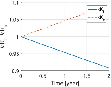
An increase in the roughness of the blade surface is the primary cause of marine PRP performance degradation [48]. This is caused by accretions of marine organisms to the metal, alloy erosion and corrosion, or combinations of these elements. The PRP decay status has been modelled by increasing the torque coefficient (Kq) and by reducing the thrust coefficient (Kt). The

correction factors used for thrust reduction,kKt, and torque increase,kKq,

have been derived from [49, 50] and reported in Figure 1.

HLL Degradation Model

0 0.5 1 1.5 2

Time [year]

0.9 0.95 1 1.05 1.1

k

K t

,

k

K q

kK_t kK_q

Figure 1: Correction factors for thrust reduction,kKt, and torque increase,kKq,

0 3 0.5

60 R t

/R

ref 1

Time [year]

2 40

Speed [knots] 1.5

20 1 0

3. From Data to Condition-Based Maintenance

3.1. Dataset Creation

In this work, authors will use the real-data validated complex numerical simulator of a Navy frigate described in Section 2 to build a realistic set of data for designing and test purposes of DDMs. This dataset will be released for the use to the research community on the widespread well-known dataset repository OpenML [43]. Currently, it can be downloaded fromhttps://cbm-anomaly-detection.smartlab.ws.

The NPS model input parameters are provided in [53] however, for clarity in this paper they are repeated verbatim here as follows:

• Speed: this parameter is controlled by the control lever. The latter can only assume a finite number of positions lpi withi ∈ {0,· · ·,9},

which in turn correspond to a finite set of possible configurations for fuel flow and blade position. Each set point is designed to reach a desired speedvi withi∈ {0,· · · ,9}:

vi= 3∗lpi[Knots], ∀i∈ {0,· · ·,9}. (1)

Note that, if the transients is not taken into account, lpi and vi are

deterministically related by a linear law. In the presented analysis the transients between different speeds have been not considered.

• As reported in Section 2.3, the PRP thrust and torque decay limit over two years of operations are:

kKt∈[0.9,1.0], kKq ∈[1.0,1.1] (2)

kKtand kKq are respectively the components which define the decay

of the torque and the thrust provided by the propeller in time. They are linearly correlated, since as the first decay of a certain quantity, the latter decay of the same quantity (1−kKt =kKq−1). For this

reason only kKt will be analysed, considering the linear dependency

between the two variables.

• The HLL decay has been modelled according to the available literature [52] as described in Section 2.3. The decay limits over two years of operations are:

• GTC decay:

kMc∈[0.95,1.0] (4)

• GT decay:

kMt∈[0.975,1.0] (5)

The performance decay functions described in Section 2.3 have been empir-ically derived as functions of the time variable solely. The real degradation behaviour of the physical asset should be defined through specific functions able to express the time dependency, the mutual interactions between the subsystems and the real operational profile. To overcome this issue, authors considered each possible combination of GTC, GT, HLL, and PRP decay status based on the described functions, and sampled the range of decays with a uniform grid characterised by a degree of precision sufficient to have a proper granularity of representation. Given the above premises, the evo-lution of the system between two important dry dock maintenance for HLL and PRP can be exhaustively and realistically explored by simulating all its possible decayed states, as all the components are decaying the same time.

The space of possible states is described via the following tuple:

(lp, kKt, kKq, kH, kMc, kMt)_i, i∈ {1,· · · ,455625} (6)

since:

lp∈ Slp={0,3,6,· · · ,27}, (7)

kKt∈ SkKt ={0.9,0.9 +0.1/14,0.09 +0.2/14,· · · ,1.0}, (8)

kKq = 2−kKt, (9)

kH ∈ SkH ={1.0,1.0 +0.2_{/14,1.0 +}0.4_{/14,· · ·,1.2}, (10)}

kMc∈ SkMc ={0.95,0.95 +0.05/14,0.95 +0.1/14,· · · ,1.0}, (11)

kMt∈ SkMt ={0.975,0.975 +0.025/14,0.975 +0.05/14,· · ·,1.0}. (12)

Note that the total number of samples 455625 is the result of making a simulation for each possible combination of decay status (15 values for GTC, 15 for GT, 15 for HLL, and 15 PRP) and speed (9 values). Once these quantities are fixed, the numerical model is run until the steady state is reached. Then, the model is able to provide all the quantities reported in Table 1. These subsets of models outputs are the same quantities that the automation system installed on-board can acquire and store.

Table 1: Measured values available from the continuous monitoring system

# Variable name Unit

1 Lever (lp) [ ]

2 Vessel speed [knots]

3 GT shaft torque [kN m]

4 GT speed [rpm]

5 PRP thrust (starboard) [N]

6 PRP thrust (port) [N]

7 Shaft torque (port) [kN m]

8 Shaft speed (port) [rpm]

9 Shaft torque (starboard) [kN m]

10 Shaft speed (starboard) [rpm]

11 HP GT exit temperature [o_C]

12 Gas generator speed [rpm]

13 Fuel flow (mf) [kg/s]

14 TIC control signal [%]

15 GTC outlet air pressure [bar]

16 GTC outlet air temperature [oC]

17 External pressure [bar]

18 HP GT exit pressure [bar]

19 TCS TIC control signal [ ]

20 Thrust coefficient (starboard) [ ]

21 PRP speed (starboard) [rps]

22 Thrust coefficient (port) [ ]

23 PRP speed (port) [rps]

24 PRP torque (port) [kN m]

3.2. Condition-Based Maintenance

This study aims at estimating the four decay variables described in the previous section, adopting different DA techniques. This section reports how the data generated can be used to create effective predictive DDMs for the CBM of an NPS.

The data described in Section 3.1 contain two sets of information: one regarding the quantities that the automation system installed on-board can acquire and store and the other one regarding the associated state of decay (efficiency coefficient) of the different NPS components (GT, GTC, HLL, and PRP).

This problem could have been straightforwardly mapped into a classi-cal multi-output regression problem, as in [31], where the aim is to predict the actual decay coefficient based on the automation data coming from the sensors installed on-board [22]. Unfortunately, this approach cannot be adopted in a real operational scenario. While the sensors’ data coming from the automation system are easy to collect, the information regarding the as-sociated state of decay is not so easy to retrieve. In fact, to circumvent this challenge to prove DDMs authors exploited a numerical model for gathering all the information and build the dataset presented in Section 3.1. In prac-tice, instead, retrieving the state of decay of the different NPS components requires the intervention of an experienced operator and, in some cases, to stop the vessel or even to put the ship in a dry dock. Moreover, data-driven regression models require a huge amount of historical data and therefore a long acquisition time.

The data described in Section 3.1 can be easily exploited to tackle this new problem as well. In fact, by thresholding kKt, kH, kMc, and kMt

the corresponding binary valued state of decay of the NPS components are obtained. In other words, if the efficiency coefficients are above or below a defined threshold, based on the accepted loss in efficiency of the NPS components, they will be tagged as “decayed” or “not decayed”. Thresh-olds were fixed according to the least affordable value of decay of the single component. Defining these thresholds is not a trivial task. Authors ap-proach is to define the maximum level of inefficiency that the operator or the shipowner is willing to tolerate before taking action and re-establish the efficiency of the system. The authors considered two years as a typical time frame between two important dry dock maintenance for HLL and PRP.

The HLL and PRP thresholds have been defined considering one year of operation. The proposed limits are just an example of the possible selection that is possible to setup to implement a CBM framework

kKt (

[0.9−0.95) decayed

[0.95−1] not decayed (13)

kH

(

(1.1−1.2] decayed

[1−1.1] not decayed (14)

As for GT and GTC, an effective time service of 2000 hours per year is considered as a reasonable operating time for these vessel types. In agree-ment with these observations authors defined the following thresholds based on the knowledge of the time domain decay functions:

kMc (

[0.95−0.98) decayed

[0.98−1] not decayed (15)

kMt (

[0.975−0.99) decayed

[0.99−1] not decayed (16)

Results will show that estimating if the decay state is acceptable or not, instead of estimating its specific state, remarkably reduces the number of samples required to find accurate DDMs. However, this quantity is still too large with respect to what can be collected in a real operational scenario.

automation system represent ordinary operating conditions corresponding to a reasonable decay state of the NPS components (GT, GTC, HLL, and PRP). Just very few times during the ship lifetime it happens that it has to operate with over-decayed components. If, for some reasons, one or more NPS components decay too fast, the corresponding automation data mea-surements will deviate from their expected behaviour. This new problem can be straightforwardly mapped into a classical outlier (novelty) detection problem [54, 36, 42] where the aim is to detect unexpected behaviour in the sensor data collected by the automation system which may correspond to an over-decayed state of an NPS components. This method does not require to know either the actual state of decay of the components, as a regression task would do, or the less detailed information about “decayed” or “not de-cayed”, as in the binary classification framework. In this case, the method just needs the sensor data collected by the automation system (see Table 1) without any supervision or feedback from the operator. These kinds of DDMs try to build a model of the “usual” operational profile of the ship and automatically detect if the sensor data collected by the automation system are “deviating too much” from the established behaviour. In our context “usual” means that the efficiency of GT, GTC, HLL, and PRP are in the acceptable range while “deviating too much” means that they are not in the acceptable range, according to Eqns. (13), (14), (15), and (16).

As for the binary classification framework, the data described in Section 3.1 can be easily exploited to tackle this problem as well. In fact, it is just necessary to keep the data corresponding to an acceptable decay state with respect to kKt, kH, kMc, and kMt and in accordance with Eqns. (13),

(14), (15), and (16). Finally, for testing and tuning the DDMs, it is possible to use just a few samples of the dataset corresponding to an unacceptable decay state. Note that these are the only samples which are costly to retrieve since they are the only ones that require the intervention of expert operators. Results will show that with just very few samples (≈ 10) of decayed state of the vessel, it is possible to obtain effective DDMs for CBM of NPS.

simplification will further reduce the amount of historical data needed to build effective CBM DDMs for NPS.

4. Machine Learning

In this section, authors will present the ML techniques adopted in order to build the CBM DDMs for NPS described in Section 2, based on the data outlined in Section 3.

Let authors consider an input space X ⊆ _Rd _{and an output space Y.}

Note that, for what concerns this paper,X takes into account the different sensors measurements, also called features, reported in Table 1, while the output spaceY depends on the particular problem identified in Section 3.2. ML techniques aim at estimating the unknown rule µ : X → Y which associates an element y∈ Y to an element x∈ X. Note that, in general, µ

can be non-deterministic. An ML technique estimatesµthrough a learning algorithmAH:Dn× F →h, characterized by its set of hyperparametersH,

which maps a series of examples of the input/output relation contained in a dataset ofnsamplesDn:{(x1, y1),· · · ,(xn, yn)}into a functionf :X → Y

chosen in a set of possible onesF.

When both xi and yi withi∈ {1,· · · , n} are available, the problems is

named supervised and consequently supervised ML technique are adopted [22]. Classification is one of the most popular examples of supervised ML problems [36]. In classification, the output space is composed of a finite set of c possibilitiesY ∈ {C1,· · ·, Cc}. Binary classification is a particular

example of classification problem whereY ∈ {±1}.

When just xi with i ∈ {1,· · · , n} are available, which means that the

associated element of the output spaceyiwithi∈ {1,· · ·, n}is not explicitly

known, it has to be assumed that “similar”xi are associated with “similar”

yi where the concept of similarity is something that needs to be defined

based on µ. In this last case, the ML problems are called unsupervised, and consequently, unsupervised ML techniques need to be adopted [55]. Anomaly (novelty, outlier) detection is a common example of unsupervised learning problem where the unknowny ∈ Y can assume only two possible values: −1 for “non-anomaly” and +1 for “anomaly” [36].

The error thatf commits in approximatingµis measured with reference to a loss function`:X ×Y×F →[0,∞). Obviously, the error thatf commits overD_n, is optimistically biased since D_n has been used, together with F, for building f itself. For this reason, another set of fresh data, composed of m samples and called test set Tm = {(xt1, y1t),· · · ,(xtm, ymt )}, needs to

the association of y_it to xt_i is again made based on µ. Moreover, both for supervised and unsupervised problems T_m must contain both xt_i ∈ X and

yt

i ∈ Y withi∈ {1,· · ·, m}to estimate the error off, while, for unsupervised

learning problems,yi withi∈ {1,· · · , n} inDn is unknown.

4.1. Measuring the Error

In this work, many state-of-the-art ML techniques will be tested and their performances will be compared to understand what is the most suited solution for building CBM DDMs for NPS.

In order to perform this analysis, authors have to define different mea-sures of error, also called indexes of performance, able to well characterize the quality of the different CBM DDMs for NPS. Once f has been chosen based onDn, it is possible to use the fresh set of dataTmin order to compute

its error based on different losses. The choice of the loss strongly depends on the problem under examination [56].

In the classification framework, the most natural choice as loss func-tion is the Hard loss one, which counts the number of misclassified samples

`H(f(x), y) = [f(x) 6= y]. Note that the Iverson bracket notation is

ex-ploited. In this work, only binary classification problems are investigated, then the Hard loss function can be expressed as `H(f(x), y) = 1−yf(x)/2.

Moreover, this measure will be also used for the anomaly detection prob-lems since, also in this case, a binary output is considered (non-anomaly or anomaly).

Based on the Hard loss it is possible to define different indexes of per-formance [57]:

• the Average Misclassifications Rate (AMR) is the mean number of misclassified samples: AMR = _m1 Pm_i=1`H(f(xti), yit);

• the Confusion Matrix, which measures four different quantities:

– TN =100_/mPm

i=1[f(xti = yti ∧yit = −1] which is the percentage

of true negative;

– TP =100_/mPm

i=1[f(xti =yit∧yit= +1] which is the percentage of

true positive;

– FN =100_/mPm

i=1[f(xti 6=yit∧yit=−1] which is the percentage of

false negative;

– FP =100_/mPm

i=1[f(xti =6 yit∧yit= +1] which is the percentage of

false positive.

4.2. Machine Learning Techniques

NPS. Moreover, authors will show how to tune their performances by tuning their hyperparameters during the so-called Model Selection (MS) phase [58, 59, 60]. Finally, authors will also check for possible spurious correlation in the data by performing the Feature Selection (FS) phase [61, 62, 63, 64, 65]. In fact, once f is built based on the different learning algorithm and has been confirmed to be a sufficiently accurate representation of µ, it can be interesting to investigate how the modelf is affected by the different features that have been exploited to buildf itself during the feature ranking procedure [61]. As authors will describe later, for some algorithms, the feature ranking procedure is a by-product of the learning process itself and allows to simply check the physical plausibility off.

4.2.1. Supervised Classification Learning Algorithms

Supervised ML techniques can be grouped into different families, accord-ing to the space of function F from which the learning algorithm chooses the particular f, the approximation of µ, based on the available data Dn.

In fact, techniques belonging to the same family, share an affineF. Among the several possible ML families, authors choose the state-of-the-art ones which are commonly adopted in real-world application, and, in each family, the best performing techniques are selected. In particular, Neural Networks (NNs), Kernel Methods (KMs), Ensemble Methods (EMs), Bayesian Meth-ods (BMs), and Lazy MethMeth-ods (LMs) are adopted.

NNs are ML techniques which combine together many simple models of a human brain neuron, called perceptrons [37], in order to build a complex network. The neurons are organized in stacked layers connected together by weights that are learned based on the available data via backpropagation [66]. The hyperparameters of an NNHNN _{are the number of layers h}

1 and

the number of neurons for each layerh2,i withi∈ {1,· · ·, h1}. Note that it

is assumed that NN with only one hidden layer hash1= 1. If the

architec-ture of the NN consists of only one hidden layer, it is called shallow (SNN) [67, 68], while, if multiple layers are staked together, the architecture is de-fined as deep (DNN) [69, 70, 71]. Extreme Learning Machines (ELMs) are a particular kind of SNN, where the weights of the first layer are randomly chosen, while the ones of the output layers are computed according to the Regularized Least Squares (RLS) principle [72, 73, 74]. The hyperparame-ters of the ELM HELM _{are the number of neurons of the hidden layer, h}

1,

and the RLS regularization hyperparameterh2 [75].

minimiz-ing the trade-off between the sum of the accuracy over the data, namely the empirical error, and the solution complexity, namely the regularization term [78, 76, 79]. The most effective KM techniques are: Kernelized Regu-larized Least Squares (KRLS), and Support Vector Machines (SVMs). The hyperparameters of the KRLS HKRLS _{are: the kernel, which in this paper}

is fixed to Gaussian Kernel for the reasons described in [80, 81], its hyper-parameter h1 and the regularization hyperparameter h2. SVM, instead, is

a classification method, which roots in the Statistical Learning Theory [22] and differs from the KRLS mainly because of its particular loss function [56]. The hyperparameters of the SVM are the same as the one of the KRLS.

EMs ML techniques rely on the fact that combining the output of several classifiers results in a much better performance than using any one of them alone [82, 40]. Random Forest (RF) [40] and Random Rotation Ensembles (RRF) [83], two popular state-of-the-art and widely adopted methods, com-bine many decision trees in order to obtain effective predictors which have limited hyperparameter sensitivity and high numerical robustness [84, 85]. Both RF and RRF have hidden hyperparameters which are arbitrarily fixed in this work because of their limited effect [86].

BMs are ML techniques where, instead of choosing a particular f ∈ F a distribution for choosing f ∈ F is defined [87]. Gaussian Processes (GP) learning algorithm is a popular BM [38] which employs a collection of Gaussians in order to compute the posterior distribution of thef(x). In fact, this algorithm defines the probability distribution of the output values as a sum of Gaussians whose variance is fixed according to the training data. The hyperparameter of the GPHGP _{is the parameter which governs}

the Gaussians widthh1.

LMs ML techniques are learning method in which the definition of f is delayed untilf(x) needs to be computed [39]. LMs approximate µ locally with respect to x. K-Nearest Neighbors (KNN) is one of the most pop-ular LM due to its implementation simplicity and effectiveness [88]. The hyperparameter of the KNN HKNN _{is the number of neighbors of x to be}

consideredh1.

4.2.2. Unsupervised Learning Algorithms for Anomaly Detection

In particular One-Class SVM (OCSVM) is a boundary-based anomaly detection method, inspired by SVM, which enclose the inlier class in a min-imum volume hypersphere by minimizing a Tikhonov regularization prob-lem, similar to the one reported for SVM framework. Like traditional SVMs, OCSVM can also be extended to non-linearly transformed spaces using the “Kernel trick” for distances. The hyperparameters OCSVM HOCSVM _are

the same as the ones of SVM.

The Global KNN (GKNN), inspired by the KNN, has been originally introduced as an unsupervised distance-based outlier detection method [89, 42]. The hyperparameter GKNNHGKNN _{is the same as the one of KNN.}

4.2.3. Model Selection

MS deals with the problem of tuning the hyperparameters of each learn-ing algorithm [60]. Several methods exist for MS purpose: resampllearn-ing meth-ods, like the well-knownk-Fold Cross Validation (KCV) [58] or the nonpara-metric Bootstrap (BTS) approach [90, 91], which represent the state-of-the-art MS approaches when targeting real-world applications. Resampling methods rely on a simple idea: the original dataset Dn is resampled once

or many (nr) times, with or without replacement, to build two independent

datasets called training, and validation sets, respectively Lr

l and Vvr, with

r ∈ {1,· · ·, nr}. Note that Lr_l ∩ Vvr = , Lrl ∪ Vvr = Dn. Then, to

se-lect the best combination the hyperparameters H in a set of possible ones H={H₁,H₂,· · · }for the algorithm AH or, in other words, to perform the MS phase, the following procedure has to be applied:

H∗ : min

H∈H

1

nr nr

X

r=1

1

v

X

(xi,yi)∈Vvr

`(AH,Lr

l(xi), yi), (17)

whereAH,Lr

l is a model built with the algorithmA with its set of hyperpa-rametersHand with the dataLr

l. Since the data inLrl are independent from

the ones in Vr

v, the idea is that H∗ should be the set of hyperparameters

which allows to achieve a small error on a data set that is independent from the training set.

Note that, for the anomaly detection problem, the algorithms do not need any label in Lr

l, consequently authors just need the labeled data for

Vr v.

If r= 1, if l and v are aprioristically set such that n=l+v, and if the resample procedure is performed without replacement, the hold out method is obtained [60]. For implementing the complete KCV, instead, it is needed to set r ≤ n_k n−n

k

k

must be done without replacement [58, 92, 60]. Finally, for implementing the BTS,l =n and Lr

l must be sampled with replacement from Dn, while

Vr

v and Ttr are sampled without replacement from the sample of Dn that

have not been sampled in Lr

l [90, 60]. Note that for the BTS procedure

r ≤ 2n_n−1

. In this paper the BTS is exploited because it represents the state-of-the-art approach [90, 60].

4.3. Feature Selection

Once the CBM NPS models are built and have been confirmed to be sufficiently accurate representation of the real decays of the components, it can be interesting to investigate how these models are affected by the different features used in the model identification phase (see Table 1).

In DA this procedure is called FS or Feature Ranking [61, 62, 63, 64, 65]. This process allows detecting if the importance of those features, that are known to be relevant from a physical perspective, is appropriately described by the different CBM NPS models. The failure of the statistical model to properly account for the relevant features might indicate poor quality in the measurements or spurious correlations. FS therefore represents an important step of model verification, since it should generate consistent results with the available knowledge of the physical system under exam.

In addition to its use for classification purposes, the EMs can also be used to perform a very stable FS procedure. The procedure is a combination of EMs, together with the permutation test [93], in order to perform the selection and the ranking of the features. In details, for every tree, two quantities are computed: the first one is the error on the out-of-bag samples as they are used during prediction, while the second one is the error on the out-of-bag samples after a random permutation of the values of variablej. These two values are then subtracted and the average of the result over all the trees in the ensemble is the raw importance score for variable j (mean decrease in accuracy). This procedure was adopted since it can be easily carried out during the main prediction process inexpensively.

5. Results

In this section, authors report the results obtained by the different meth-ods applied to the CBM of the main components of an NPS, in classification, and novelty detection frameworks, as described in Section 2, based on the data described in Section 3.

Secondly, authors attempted to solve the same problem in an unsupervised fashion by modelling the problem as a novelty detection one in order to further reduce the necessity of labeled data (ANOMALY-PROB).

The dataset considered in Section 3.2 was divided into training and test set, respectively D_n and T_m, as reported in Section 4. Moreover, different dimensions of the training setn∈ {10,24,55,130,307,722,1700,4000}were considered. These dimensions were derived by considering 8 values on a logarithmic scale from 10 to 4000, to analyse the behaviour of the predictive models in different conditions.

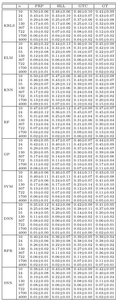
For each supervised classification ML technique, the BTS MS procedure was performed withr= 1000, as described in Section 4.2.3. Here-below, the list of hyperparameters tested during the MS, with their respective intervals, is reported:

1. DNN: the set of hyperparameters isHDN N _={h

1, h2,1,· · · , h2,h1}and authors chose it inHDNN={1,3,5,7,10} × {10,101.2· · · ,103} × · · · × {10,101.2· · · ,103};

2. SNN: the set of hyperparameters isHSN N _={h

1} and authors chose

it inHSNN={1,3,5,7,10};

3. ELM: the set of hyperparameters is HELM _{= {h}

1, h2} and authors

chose it inHELM ={10,101.2,· · · ,103} × {10−2,10−1.5· · ·,102}; 4. SVM: the set of hyperparameters is HSV M _{= {h}

1, h2} and authors

chose it inHSVM ={10−2,10−1.4,· · · ,103} × {10−2,10−1.4· · · ,103}; 5. KRLS: the set of hyperparameters is HKRLS _={h

1, h2} and authors

chose it inHKRLS ={10−2,10−1.4,· · · ,103} × {10−2,10−1.4,· · ·,103}; 6. KNN: the set of hyperparameters isHKN N _={h

1}and authors chose

it inHKNN={1,3,7,13,27,51};

7. GP: the set of hyperparameters is HGP _={h

1} and authors chose it

inHGP={100_,100.3_{,· · · ,10}3_};

When RF is exploited, also the FS phase is performed to understand how the data-driven model combines the different features in order to predict the decay state of each component.

Similarly to the supervised learning task, in the unsupervised case differ-ent dimensions of the training set were consideredn∈ {1500,2000,3000,4000}

and the MS procedure was performed as follows:

1. OCSVM: the set of hyperparameters is HOCSV M _{= {h}

1, h2} and

au-thors chose it inHOCSVM={10−4,10−3.7,· · ·,103}×{10−4,10−3.8,· · · ,

10−1.0_};

2. GKNN: the set of hyperparameters is HGKN N _{= {h}

1} and authors

chose it inHGKNN={1,3,7,13,27,51}; The Vr

test the possibility of building an efficient model with a few labeled samples. Note that, also in this case, the BTS MS procedure is adopted withr = 1000 and that the labels are only needed in Vr

v and not in Lrl as described in

Section 4.2.3.

The performances of each model are measured according to the metrics described in Section 4.1. Each experiment was performed 10 times in order to obtain statistical relevant result, and the t-student 95% confidence inter-val is reported when space in the table was available without compromising their readability.

For SNN and DNN the Python Keras library [94] has been exploited. For ELM, SVM, KRLS, KNN, and GKNN a custom R implementation has been developed. For RF the R package of [95] has been exploited. For RFE the implementation of [83] has been exploited. For GP the R package of [96] has been exploited. For OCSVM the R package of [97] has been exploited.

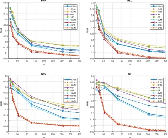
5.1. CLASS-PROB

In this section, the results on the CLASS-PROB are reported. In Figures 3 the AMR of the models learned with the different algorithms is reported, when varying n and for the four main NPS components. In Figures 4 the AMR of the DNN (the best performing model) is reported, when varyingn

and for the four main NPS components.

From the different tables and figures it is possible to observe that: • the larger is n the better performances are achieved by the learned

models (see Figure 3) and the models learned with ELM, SNN, and especially DNN generally show the best performances (see Figure 3); • as expected, to achieve a reasonable AMR a smaller number of samples

is needed with respect to a regression-based approach not feasible in practice.

0 50 100 150 200 250 300 350 400 n 0.05 0.1 0.15 0.2 0.25 0.3 0.35 0.4 0.45 0.5 0.55 AMR PRP KRLS ELM KNN RF GP SVM DNN RFR SNN

0 50 100 150 200 250 300 350 400

n 0.05 0.1 0.15 0.2 0.25 0.3 0.35 0.4 0.45 0.5 AMR HLL KRLS ELM KNN RF GP SVM DNN RFR SNN

0 50 100 150 200 250 300 350 400

n 0 0.05 0.1 0.15 0.2 0.25 0.3 0.35 0.4 0.45 0.5 AMR GTC KRLS ELM KNN RF GP SVM DNN RFR SNN

0 50 100 150 200 250 300 350 400

n 0.05 0.1 0.15 0.2 0.25 0.3 0.35 0.4 0.45 0.5 AMR GT KRLS ELM KNN RF GP SVM DNN RFR SNN

Figure 3: CLASS-PROB: AMR of the models learned with the different algorithms when varyingnand for the four main NPS components.

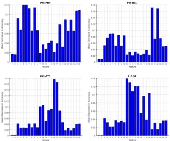
highest predictive power, nominally GTC outlet air temperature, External pressure, and HP GT exit temperature features (16, 17 and 11). Finally, for the GT component prediction, several features are necessary, also this case is in line with engineering state-of-the-art knowledge [53]. These re-sults indicate that, from a data driven perspective, the decay state of each component influences different phases of the NPS behavior.

0 50 100 150 200 250 300 350 400 n 0.1 0.15 0.2 0.25 0.3 0.35 0.4 0.45 0.5 0.55 AMR PRP HLL GTC GT

Figure 4: CLASS-PROB: AMR of the models learned with DNN when varyingnfor the four main NPS components.

1 234 567 8910 11 12 13 14 15 16 17 18 19 20 21 22 23 24 25

feature 0 0.02 0.04 0.06 0.08 0.1 0.12

Mean Decrease in Accuracy

P15:PRP

123 456 78910 11 12 13 14 15 16 17 18 19 20 21 22 23 24 25

feature 0 0.02 0.04 0.06 0.08 0.1 0.12 0.14 0.16 0.18

Mean Decrease in Accuracy

P15:HLL

1 234 567 8910 11 12 13 14 15 16 17 18 19 20 21 22 23 24 25

feature 0 0.02 0.04 0.06 0.08 0.1 0.12 0.14 0.16 0.18 0.2

Mean Decrease in Accuracy

P15:GTC

123 456 78910 11 12 13 14 15 16 17 18 19 20 21 22 23 24 25

feature 0 0.02 0.04 0.06 0.08 0.1 0.12 0.14

Mean Decrease in Accuracy

P15:GT

v PRP HLL GTC GT

OCSVM

10 0.08±0.08 0.07±0.09 0.05±0.07 0.11±0.06 20 0.08±0.10 0.08±0.07 0.10±0.07 0.09±0.06 30 0.08±0.07 0.12±0.08 0.10±0.07 0.09±0.03

GKNN

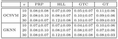
10 0.07±0.07 0.07±0.09 0.04±0.07 0.10±0.06 20 0.08±0.10 0.08±0.07 0.08±0.07 0.07±0.06 30 0.08±0.07 0.12±0.08 0.08±0.08 0.08±0.03

Table 2: ANOMALY-PROB: AMR of the models learned with the different algorithms (OCSVM and GKNN) when l = 4000 and v∈ {10,20,30} and for the four main NPS components.

5.2. ANOMALY-PROB

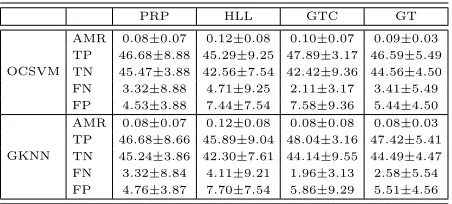
In this section the results on the ANOMALY-PROB are reported. In Table 2, for PRP, HLL, GTC, and GT, the AMR of the models learned with the different algorithms (OCSVM and GKNN) is reported, when the number of unlabelled samples in the learning set is l= 4000 and when varying the number of labeled samples in the validation set v ∈ {10,20,30} (half posi-tively and half negaposi-tively labeled). In Table 3, respecposi-tively for PRP, HLL, GTC, and GT, the AMR of the models learned with the different algorithms is reported, whenv = 30 and whenl∈ {1500,2000,3000,4000}. In Table 4, for PRP, HLL, GTC, and GT, the different indexes of performances (AMR, TP, TN, FP, and FN) of the models learned with the different algorithms are reported whenn= 4000 andv= 30.

From the tables it is possible to observe that:

• both OCSVM and GKNN perform quite well on the problem and there is no clear winner;

• changing l or v does not remarkably affect the performance of the models;

• with just few labeled samples, around 10, it is possible to obtain satis-fying accuracies and this is quite a remarkable result, since 10 samples can be easily manually labeled by an expert operator;

• in some cases, the mean value of the reported AMR increases instead of decreasing when the number of training samples increases; as a fact, this value is subject to statistical variation in the data whose variance in the results can be considered acceptable from a statistical point of view. Note also that the number of validation samples is very limited and this high variance is also justified by this fact;

n PRP HLL GTC GT

OCSVM

1500 0.09±0.04 0.14±0.09 0.11±0.09 0.08±0.03 2000 0.12±0.10 0.11±0.04 0.10±0.04 0.11±0.13 3000 0.08±0.06 0.11±0.04 0.13±0.17 0.08±0.05 4000 0.08±0.07 0.12±0.08 0.10±0.07 0.09±0.03

GKNN

1500 0.09±0.04 0.12±0.09 0.10±0.09 0.06±0.03 2000 0.11±0.11 0.12±0.04 0.08±0.04 0.08±0.13 3000 0.07±0.06 0.10±0.04 0.12±0.16 0.09±0.04 4000 0.08±0.07 0.12±0.08 0.08±0.08 0.08±0.03

Table 3: ANOMALY-PROB: AMR of the models learned with the different algorithms (OCSVM and GKNN) whenl∈ {1500,2000,3000,4000}andv= 30 and for the four main NPS components.

PRP HLL GTC GT

OCSVM

AMR 0.08±0.07 0.12±0.08 0.10±0.07 0.09±0.03 TP 46.68±8.88 45.29±9.25 47.89±3.17 46.59±5.49 TN 45.47±3.88 42.56±7.54 42.42±9.36 44.56±4.50 FN 3.32±8.88 4.71±9.25 2.11±3.17 3.41±5.49 FP 4.53±3.88 7.44±7.54 7.58±9.36 5.44±4.50

GKNN

AMR 0.08±0.07 0.12±0.08 0.08±0.08 0.08±0.03 TP 46.68±8.66 45.89±9.04 48.04±3.16 47.42±5.41 TN 45.24±3.86 42.30±7.61 44.14±9.55 44.49±4.47 FN 3.32±8.84 4.11±9.21 1.96±3.13 2.58±5.54 FP 4.76±3.87 7.70±7.54 5.86±9.29 5.51±4.56

Table 4: ANOMALY-PROB: the different indexes of performances (AMR, TP, TN, FP, and FN) of the models learned with the different algorithms (OCSVM and GKNN) when

6. Conclusions

The maintenance of the several components of a Ship Propulsion Sys-tems is an onerous activity, which needs to be efficiently programmed by a shipbuilding company to save time and money. The replacement policies of these components can be planned in a Condition-Based fashion, by predict-ing their decay state and thus proceed to substitution only when needed. In this paper, authors proposed several Data Analysis supervised and unsu-pervised techniques for the Condition-Based Maintenance of a naval vessel, characterised by a combined diesel-electric and gas propulsion plant. The propulsion plant has been modelled using the state-of-the-art simulation techniques available in the literature [44, 47]. The dataset used to bench-mark the proposed data-driven approaches has been created using a realistic simulator of Frigate validated and fine-tuned during sea trials. The model has been designed to work in calm water scenario, and measurement uncer-tainties have not been taken into account. Within the mentioned limitations of the numerical model, the authors are confident that the results shown are in line with the real behaviour of the system. The authors considered the case in which GTC, GT, HLL, and PRP NPS components decay at the same time, to provide a realistic simulation environment.

The proposed analysis considered contexts where the collection of vast amounts of labelled data containing the exact decay state of the components is unfeasible. In fact, the collection of labelled data requires a drydocking of the ship and the intervention of expert operators, which is usually an infrequent event. As a result, authors focused on methods which could allow only a minimal feedback from naval specialists, thus simplifying the dataset collection phase. In particular, supervised Data Analysis techniques allowed to reach an average percentage error of 1%±2% adopting 4000 labelled samples respectively for all PRP, HLL, GTC, and GT. On the other hand, the non-supervised techniques exploited could reach an average value of 8%±5% error adopting only 10 labelled data overall. To reach the same average error percentage, the obtained supervised models required at least a number of labelled data between 130 and 307, thus requiring a higher amount of information for learning a performing model. Clearly, supervised models could reach a lower error rate with respect to unsupervised ones (1%±2%), adopting a higher amount of labelling training data, but such a difference in accuracy is obtained through higher costs for dataset collection, which cannot be sustained in most cases.

to the ones obtained with supervised techniques present in literature. These models can be adopted for real-time applications directly on-board, to easily and quickly identify maintenance necessities.

Appendix A. CLASS-PROB Extended Results

In this section, the results for the CLASS-PROB, from which Figures 3 and 4 were derived, are extensively reported. In Table A.5, respectively for PRP, HLL, GTC, and GT, the AMR of the models learned with the different algorithms (DNN, SNN, ELM, SVM, KRLS, KNN, and GP) is reported, when varying n. In Table A.6, instead, respectively for PRP, HLL, GTC, and GT, the different indexes of performances (AMR, TP, TN, FP, and FN) of the models learned with the different algorithms are reported, whenn is the largest possible.

Appendix B. References

[1] R. Ahmad, S. Kamaruddin, An overview of time-based and condition-based maintenance in industrial application, Computers & Industrial Engineering 63 (1) (2012) 135–149.

[2] S. K. Pinjala, L. Pintelon, A. Vereecke, An empirical investigation on the relationship between business and maintenance strategies, Interna-tional journal of production economics 104 (1) (2006) 214–229.

[3] A. H. C. Tsang, Condition-based maintenance: tools and decision mak-ing, Journal of Quality in Maintenance Engineering 1 (3) (1995) 3–17.

[4] R. Dekker, P. A. Scarf, On the impact of optimisation models in main-tenance decision making: the state of the art, Reliability Engineering & System Safety 60 (2) (1998) 111–119.

[5] S. Takata, F. Kirnura, F. A. M. van Houten, E. Westkamper, M. Sh-pitalni, D. Ceglarek, J. Lee, Maintenance: changing role in life cycle management, CIRP Annals-Manufacturing Technology 53 (2) (2004) 643–655.

n PRP HLL GTC GT

KRLS

10 0.50±0.06 0.48±0.06 0.46±0.10 0.44±0.09 24 0.43±0.10 0.43±0.10 0.43±0.07 0.43±0.07 55 0.29±0.06 0.25±0.07 0.37±0.06 0.42±0.08 130 0.17±0.05 0.17±0.06 0.25±0.12 0.32±0.09 307 0.13±0.02 0.11±0.02 0.13±0.03 0.19±0.03 722 0.10±0.02 0.07±0.02 0.08±0.03 0.12±0.03 1700 0.06±0.01 0.04±0.02 0.05±0.02 0.07±0.02 4000 0.03±0.01 0.02±0.01 0.04±0.02 0.05±0.01

ELM

10 0.40±0.22 0.44±0.13 0.46±0.16 0.45±0.09 24 0.28±0.14 0.31±0.18 0.31±0.20 0.42±0.16 55 0.19±0.08 0.23±0.09 0.16±0.07 0.22±0.07 130 0.12±0.05 0.11±0.05 0.08±0.03 0.12±0.03 307 0.09±0.04 0.06±0.03 0.06±0.02 0.07±0.01 722 0.05±0.04 0.04±0.02 0.05±0.02 0.05±0.02 1700 0.03±0.01 0.03±0.01 0.03±0.01 0.03±0.01 4000 0.01±0.01 0.01±0.01 0.01±0.01 0.02±0.02

KNN

10 0.50±0.07 0.47±0.06 0.46±0.10 0.43±0.08 24 0.46±0.08 0.43±0.15 0.43±0.08 0.43±0.07 55 0.29±0.07 0.28±0.12 0.39±0.05 0.42±0.08 130 0.21±0.05 0.21±0.06 0.30±0.03 0.40±0.07 307 0.17±0.02 0.15±0.02 0.24±0.04 0.33±0.04 722 0.15±0.03 0.12±0.02 0.18±0.03 0.26±0.02 1700 0.13±0.02 0.10±0.02 0.13±0.02 0.20±0.02 4000 0.09±0.01 0.07±0.01 0.10±0.02 0.15±0.02

RF

10 0.47±0.07 0.43±0.12 0.47±0.09 0.47±0.07 24 0.40±0.12 0.36±0.15 0.45±0.07 0.45±0.04 55 0.31±0.08 0.25±0.06 0.41±0.04 0.45±0.03 130 0.19±0.04 0.19±0.05 0.31±0.06 0.38±0.04 307 0.13±0.04 0.12±0.04 0.21±0.05 0.30±0.04 722 0.07±0.02 0.07±0.02 0.13±0.01 0.21±0.03 1700 0.04±0.02 0.04±0.01 0.09±0.02 0.13±0.02 4000 0.02±0.01 0.02±0.01 0.06±0.02 0.08±0.02

GP

10 0.49±0.05 0.47±0.07 0.46±0.07 0.44±0.05 24 0.42±0.11 0.40±0.11 0.42±0.07 0.45±0.09 55 0.29±0.05 0.27±0.05 0.37±0.04 0.44±0.07 130 0.20±0.05 0.20±0.03 0.30±0.03 0.39±0.08 307 0.17±0.02 0.14±0.03 0.22±0.02 0.32±0.06 722 0.13±0.03 0.11±0.03 0.15±0.03 0.24±0.04 1700 0.11±0.02 0.07±0.02 0.10±0.03 0.17±0.03 4000 0.08±0.01 0.04±0.01 0.07±0.02 0.11±0.02

SVM

10 0.46±0.06 0.46±0.07 0.44±0.11 0.43±0.10 24 0.40±0.11 0.41±0.11 0.41±0.07 0.40±0.08 55 0.27±0.06 0.24±0.07 0.35±0.07 0.41±0.09 130 0.17±0.06 0.17±0.07 0.23±0.14 0.31±0.10 307 0.13±0.03 0.11±0.02 0.12±0.03 0.18±0.04 722 0.10±0.02 0.07±0.02 0.07±0.03 0.11±0.03 1700 0.06±0.02 0.04±0.02 0.05±0.02 0.07±0.02 4000 0.03±0.01 0.02±0.01 0.03±0.02 0.05±0.01

DNN

10 0.35±0.12 0.42±0.08 0.42±0.09 0.41±0.05 24 0.25±0.08 0.28±0.10 0.28±0.11 0.37±0.09 55 0.18±0.05 0.20±0.05 0.14±0.04 0.20±0.04 130 0.11±0.03 0.09±0.02 0.08±0.02 0.11±0.02 307 0.08±0.02 0.06±0.02 0.05±0.01 0.06±0.01 722 0.04±0.02 0.04±0.01 0.04±0.01 0.04±0.01 1700 0.02±0.01 0.02±0.01 0.02±0.01 0.03±0.01 4000 0.01±0.00 0.01±0.01 0.01±0.00 0.02±0.01

RFR

10 0.40±0.04 0.36±0.07 0.39±0.05 0.39±0.04 24 0.33±0.06 0.30±0.08 0.38±0.04 0.38±0.02 55 0.26±0.04 0.22±0.03 0.35±0.02 0.40±0.02 130 0.16±0.02 0.17±0.03 0.27±0.03 0.34±0.02 307 0.11±0.02 0.11±0.02 0.19±0.03 0.26±0.02 722 0.06±0.01 0.06±0.01 0.11±0.01 0.19±0.02 1700 0.04±0.01 0.03±0.01 0.07±0.01 0.11±0.01 4000 0.02±0.01 0.02±0.01 0.05±0.01 0.07±0.01

SNN

10 0.38±0.12 0.43±0.08 0.43±0.09 0.42±0.05 24 0.25±0.08 0.30±0.10 0.29±0.10 0.40±0.09 55 0.19±0.05 0.22±0.05 0.16±0.04 0.21±0.04 130 0.12±0.03 0.10±0.02 0.08±0.02 0.11±0.02 307 0.08±0.02 0.06±0.02 0.06±0.01 0.07±0.01 722 0.04±0.02 0.04±0.01 0.04±0.01 0.04±0.01 1700 0.02±0.01 0.02±0.01 0.03±0.01 0.03±0.01 4000 0.01±0.00 0.01±0.01 0.01±0.00 0.02±0.01

PRP HLL GTC GT

KRLS

AMR 0.03±0.01 0.02±0.01 0.04±0.01 0.05±0.00 TP 45.11±1.10 45.68±1.79 58.06±1.67 57.29±1.37 TN 51.72±1.02 52.33±1.97 38.31±1.45 37.77±1.50 FN 1.64±0.39 0.84±0.28 1.96±0.74 2.81±0.55 FP 1.53±0.47 1.15±0.35 1.67±0.49 2.13±0.37

ELM

AMR 0.01±0.00 0.01±0.01 0.01±0.00 0.02±0.01 TP 45.05±1.87 46.32±0.85 60.18±1.14 57.51±1.80 TN 53.60±1.67 52.22±1.08 38.33±1.23 40.20±1.53 FN 0.80±0.31 0.64±0.30 0.73±0.24 1.94±0.75 FP 0.55±0.22 0.82±0.41 0.76±0.31 0.35±0.27

KNN

AMR 0.09±0.01 0.07±0.01 0.10±0.01 0.15±0.01 TP 42.06±0.63 43.10±1.75 55.23±1.68 52.65±1.70 TN 48.46±1.03 49.56±1.93 34.92±1.53 31.96±1.81 FN 4.69±0.51 3.42±0.53 4.79±0.71 7.45±0.68 FP 4.79±0.59 3.92±0.40 5.06±0.79 7.94±0.82

RF

AMR 0.02±0.01 0.02±0.01 0.06±0.01 0.08±0.01 TP 45.81±1.90 45.70±1.47 57.17±1.01 56.31±1.53 TN 52.03±1.68 51.89±1.26 37.31±1.01 35.78±1.61 FN 1.23±0.42 1.29±0.37 2.52±0.39 3.50±0.77 FP 0.93±0.36 1.12±0.48 3.00±0.73 4.41±0.73

GP

AMR 0.08±0.01 0.04±0.01 0.07±0.01 0.11±0.01 TP 42.33±0.84 44.17±1.94 57.43±1.55 57.07±1.51 TN 49.99±0.91 51.55±1.90 35.71±1.32 32.39±1.45 FN 4.42±0.67 2.35±0.85 2.59±0.74 3.03±0.63 FP 3.26±0.86 1.93±0.51 4.27±0.73 7.51±1.03

SVM

AMR 0.03±0.01 0.02±0.01 0.03±0.01 0.05±0.00 TP 45.15±1.21 45.70±1.95 58.16±1.90 57.36±1.48 TN 51.79±1.13 52.43±2.15 38.37±1.57 37.95±1.65 FN 1.60±0.42 0.82±0.30 1.86±0.83 2.74±0.59 FP 1.46±0.53 1.05±0.39 1.61±0.53 1.95±0.39

DNN

AMR 0.01±0.00 0.01±0.01 0.01±0.00 0.02±0.01 TP 45.10±2.08 46.40±0.96 60.25±1.20 57.65±2.02 TN 53.63±1.83 52.30±1.23 38.40±1.38 40.24±1.75 FN 0.75±0.35 0.56±0.34 0.66±0.26 1.80±0.85 FP 0.52±0.25 0.74±0.45 0.69±0.34 0.31±0.31

RFR

AMR 0.02±0.01 0.02±0.01 0.05±0.01 0.07±0.01 TP 46.05±2.12 45.96±1.63 57.56±1.08 56.68±1.64 TN 52.21±1.88 52.05±1.43 37.70±1.07 36.45±1.72 FN 0.99±0.48 1.03±0.39 2.13±0.45 3.13±0.88 FP 0.75±0.40 0.96±0.53 2.61±0.83 3.74±0.78

SNN

AMR 0.01±0.00 0.01±0.01 0.01±0.00 0.02±0.01 TP 45.10±2.00 46.33±0.93 60.19±1.25 57.56±1.89 TN 53.64±1.90 52.25±1.17 38.36±1.41 40.20±1.63 FN 0.75±0.34 0.63±0.32 0.72±0.28 1.89±0.79 FP 0.51±0.25 0.79±0.47 0.73±0.34 0.35±0.29

[7] Y. Peng, M. Dong, M. J. Zuo, Current status of machine prognostics in condition-based maintenance: a review, The International Journal of Advanced Manufacturing Technology 50 (1-4) (2010) 297–313.

[8] N. P. Kyrtatos, E. Tzanos, J. Coustas, D. Vastarouhas, E. Rizos, Ship-board engine performance assessment by comparing actual measured data to nominal values produced by detailed engine simulations, in: Proceedings, 2010.

[9] A. J. M. Goossens, R. J. I. Basten, Exploring maintenance policy se-lection using the analytic hierarchy process; an application for naval ships, Reliability Engineering & System Safety 142 (2015) 31–41.

[10] A. Widodo, B. Yang, Support vector machine in machine condition monitoring and fault diagnosis, Mechanical systems and signal process-ing 21 (6) (2007) 2560–2574.

[11] R. K. Mobley, An introduction to predictive maintenance, Butterworth-Heinemann, 2002.

[12] G. B. Q. Management, S. S. Committee, B. S. Institution, British Stan-dard Glossary of Maintenance Management Terms in Terotechnology, British Standards Institution, 1984.

[13] G. Budai-Balke, Operations research models for scheduling railway in-frastructure maintenance, Rozenberg Publishers, 2009.

[14] A. E. B. Abu-Elanien, M. M. A. Salama, Asset management techniques for transformers, Electric power systems research 80 (4) (2010) 456–464.

[15] R. Kothamasu, S. H. Huang, Adaptive mamdani fuzzy model for condition-based maintenance, Fuzzy Sets and Systems 158 (24) (2007) 2715–2733.

[16] J. T. Selvik, T. Aven, A framework for reliability and risk centered maintenance, Reliability Engineering & System Safety 96 (2) (2011) 324–331.

[17] L. Mann, A. Saxena, G. M. Knapp, Statistical-based or condition-based preventive maintenance?, Journal of Quality in Maintenance Engineer-ing 1 (1) (1995) 46–59.

[19] A. Ghasemi, S. Yacout, M. S. Ouali, Parameter estimation methods for condition-based maintenance with indirect observations, IEEE Trans-actions on reliability 59 (2) (2010) 426–439.

[20] A. K. S. Jardine, D. Banjevic, M. Wiseman, S. Buck, T. Joseph, Opti-mizing a mine haul truck wheel motors? condition monitoring program use of proportional hazards modeling, Journal of quality in Maintenance Engineering 7 (4) (2001) 286–302.

[21] G. S. Linoff, M. J. A. Berry, Data mining techniques: for market-ing, sales, and customer relationship management, John Wiley & Sons, 2011.

[22] V. N. Vapnik, Statistical learning theory, Wiley New York, 1998.

[23] L. Gy¨orfi, M. Kohler, A. Krzyzak, H. Walk, A distribution-free theory of nonparametric regression, Springer Science & Business Media, 2006.

[24] L. R. Newton, Data-logging in practical science: research and reality, International Journal of Science Education 22 (12) (2000) 1247–1259.

[25] A. K. S. Jardine, D. Lin, D. Banjevic, A review on machinery diagnos-tics and prognosdiagnos-tics implementing condition-based maintenance, Me-chanical systems and signal processing 20 (7) (2006) 1483–1510.

[26] S. Poyhonen, P. Jover, H. Hyotyniemi, Signal processing of vibrations for condition monitoring of an induction motor, in: Symposium on Control, Communications and Signal Processing, 2004.

[27] C. Bunks, D. McCarthy, T. Al-Ani, Condition-based maintenance of machines using hidden markov models, Mechanical Systems and Signal Processing 14 (4) (2000) 597–612.

[28] S. Simani, C. Fantuzzi, R. Patton, Model-based Fault Diagnosis in Dy-namic Systems Using Identification Techniques, Springer-Verlag Lon-don, 2003.

[29] T. Palm´e, P. Breuhaus, M. Assadi, A. Klein, M. Kim, New alstom monitoring tools leveraging artificial neural network technologies, in: Turbo Expo: Turbine Technical Conference and Exposition, 2011.

[31] A. Coraddu, L. Oneto, A. Ghio, S. Savio, D. Anguita, M. Figari, Ma-chine learning approaches for improving condition-based maintenance of naval propulsion plants, Proceedings of the Institution of Mechanical Engineers Part M: Journal of Engineering for the Maritime Environ-ment 230 (1) (2016) 136–153.

[32] T. S. Akinfiev, M. A. Armada, R. Fernandez, Nondestructive testing of the state of a ship’s hull with an underwater robot, Russian Journal of Nondestructive Testing 44 (9) (2008) 626–633.

[33] S. Bagavathiappan, B. B. Lahiri, T. Saravanan, J. Philip, T. Jayaku-mar, Infrared thermography for condition monitoring-a review, Infrared Physics & Technology 60 (2013) 35–55.

[34] O. C. Basurko, Z. Uriondo, Condition-based maintenance for medium speed diesel engines used in vessels in operation, Applied Thermal En-gineering 80 (2015) 404–412.

[35] I. Lazakis, K. Dikis, A. L. Michala, G. Theotokatos, Advanced ship sys-tems condition monitoring for enhanced inspection, maintenance and decision making in ship operations, Transportation Research Procedia 14 (2016) 1679–1688.

[36] J. Shawe-Taylor, N. Cristianini, Kernel methods for pattern analysis, Cambridge university press, 2004.

[37] F. Rosenblatt, The perceptron: a probabilistic model for information storage and organization in the brain., Psychological review 65 (6) (1958) 386.

[38] C. E. Rasmussen, Gaussian processes for machine learning, in: Gaussian Processes for Machine Learning, 2006.

[39] W. Duch, Similarity-based methods: a general framework for classifica-tion, approximation and associaclassifica-tion, Control and Cybernetics 29 (4).

[40] L. Breiman, Random forests, Machine learning 45 (1) (2001) 5–32.

[41] M. Markou, S. Singh, Novelty detection: a review, Signal processing 83 (12) (2003) 2481–2497.

[43] J. Vanschoren, J. N. van Rijn, B. Bischl, L. Torgo, Openml: Networked science in machine learning, SIGKDD Explorations 15 (2) (2013) 49–60.

[44] M. Altosole, G. Benvenuto, M. Figari, U. Campora, Real-time simula-tion of a cogag naval ship propulsion system, Journal of Engineering for the Maritime Environment 223 (1) (2009) 47–62.

[45] A. P. Tarabrin, V. A. Schurovsky, A. I. Bodrov, J. P. Stalder, An anal-ysis of axial compressor fouling and a blade cleaning method, Journal of Turbomachinery 120 (2) (1998) 256–261.

[46] C. B. Meher-Homji, A. B. Focke, M. B. Wooldridge, Fouling of axial flow compressors - causes, effects, detection, and control, in: Eighteenth Turbomachinery Symposium, 1989.

[47] M. Altosole, U. Campora, M. Martelli, M. Figari, Performance decay analysis of a marine gas turbine propulsion system, Journal of Ship Research 58 (3) (2014) 117–129.

[48] Y. S. Khor, Q. Xiao, Cfd simulations of the effects of fouling and an-tifouling, Ocean Engineering 38 (10) (2011) 1065–1079.

[49] M. Atlar, E. J. Glover, M. Candries, R. J. Mutton, C. D. Anderson, The effect of a foul release coating on propeller performance, in: Marine Science and Technology for Environmental Sustainability, 2002.

[50] B. Wan, E. Nishikswa, M. Uchida, The experiment and numerical calcu-lation of propeller performance with surface roughness effects, Journal of the Kansai Society of Naval Architects, Japan 2002 (238) (2002) 49–54.

[51] A. Lindholdt, K. Dam-Johansen, S. M. Olsen, D. M. Yebra, S. Kiil, Effects of biofouling development on drag forces of hull coatings for ocean-going ships: a review, Journal of Coatings Technology and Re-search 12 (3) (2015) 315–444.

[52] J. B. Hadler, C. J. Wilson, A. L. Beal, Ship standardisation trial per-formance and correlation with model predictions, in: The Society of Naval Architects and Marine Engineers, 1962.

[54] D. M. Hawkins, Identification of outliers, Springer, 1980.

[55] T. Hastie, R. Tibshirani, J. Friedman, Unsupervised learning, in: The elements of statistical learning, 2009.

[56] L. Rosasco, E. De Vito, A. Caponnetto, M. Piana, A. Verri, Are loss functions all the same?, Neural Computation 16 (5) (2004) 1063–1076.

[57] D. M. Powers, Evaluation: from precision, recall and f-measure to roc, informedness, markedness and correlation, Journal of Machine Learning Technologies 2 (1) (2011) 37–63.

[58] R. Kohavi, et al., A study of cross-validation and bootstrap for accuracy estimation and model selection, in: International Joint Conference on Artificial Intelligence, 1995.

[59] P. L. Bartlett, S. Boucheron, G. Lugosi, Model selection and error es-timation, Machine Learning 48 (1-3) (2002) 85–113.

[60] D. Anguita, A. Ghio, L. Oneto, S. Ridella, In-sample and out-of-sample model selection and error estimation for support vector machines, IEEE Transactions on Neural Networks and Learning Systems 23 (9) (2012) 1390–1406.

[61] I. Guyon, A. Elisseeff, An introduction to variable and feature selection, The Journal of Machine Learning Research 3 (2003) 1157–1182.

[62] J. Friedman, T. Hastie, R. Tibshirani, The elements of statistical learn-ing, Springer series in statistics Springer, Berlin, 2001.

[63] Y. W. Chang, C. J. Lin, Feature ranking using linear svm., in: WCCI Causation and Prediction Challenge, 2008.

[64] H. Yoon, K. Yang, C. Shahabi, Feature subset selection and feature ranking for multivariate time series, IEEE transactions on knowledge and data engineering 17 (9) (2005) 1186–1198.

[65] S. J. Hong, Use of contextual information for feature ranking and dis-cretization, IEEE Transactions on Knowledge and Data Engineering 9 (5) (1997) 718–730.

[67] G. Cybenko, Approximation by superpositions of a sigmoidal function, Mathematics of Control, Signals, and Systems (MCSS) 2 (4) (1989) 303–314.

[68] C. M. Bishop, Neural networks for pattern recognition, Oxford univer-sity press, 1995.

[69] G. E. Hinton, S. Osindero, Y. W. Teh, A fast learning algorithm for deep belief nets, Neural computation 18 (7) (2006) 1527–1554.

[70] Y. Bengio, Learning deep architectures for ai, Foundations and trends® in Machine Learning 2 (1) (2009) 1–127.

[71] Y. Bengio, A. Courville, P. Vincent, Representation learning: A re-view and new perspectives, IEEE transactions on pattern analysis and machine intelligence 35 (8) (2013) 1798–1828.

[72] G. Huang, G.-B. Huang, S. Song, K. You, Trends in extreme learning machines: A review, Neural Networks 61 (2015) 32–48.

[73] G. B. Huang, Q. Y. Zhu, C. K. Siew, Extreme learning machine: theory and applications, Neurocomputing 70 (1) (2006) 489–501.

[74] E. Cambria, G.-B. Huang, Extreme learning machines, IEEE Intelligent Systems 28 (6) (2013) 30–59.

[75] G.-B. Huang, Q.-Y. Zhu, C.-K. Siew, Extreme learning machine: a new learning scheme of feedforward neural networks, in: IEEE International Joint Conference on Neural Networks, 2004.

[76] N. Cristianini, J. Shawe-Taylor, An introduction to support vector ma-chines and other kernel-based learning methods, Cambridge university press, 2000.

[77] B. Scholkopf, The kernel trick for distances, in: Advances in neural information processing systems, 2001.

[78] R. Rifkin, G. Yeo, T. Poggio, Regularized least-squares classification, Nato Science Series Sub Series III Computer and Systems Sciences 190 (2003) 131–154.

[80] S. S. Keerthi, C. J. Lin, Asymptotic behaviors of support vector ma-chines with gaussian kernel, Neural computation 15 (7) (2003) 1667– 1689.

[81] L. Oneto, A. Ghio, S. Ridella, D. Anguita, Support vector machines and strictly positive definite kernel: The regularization hyperparameter is more important than the kernel hyperparameters, in: IEEE Interna-tional Joint Conference on Neural Networks, 2015.

[82] P. Germain, A. Lacasse, F. Laviolette, M. Marchand, J. F. Roy, Risk bounds for the majority vote: From a pac-bayesian analysis to a learn-ing algorithm, The Journal of Machine Learnlearn-ing Research 16 (1) (2015) 787–860.

[83] R. Blaser, P. Fryzlewicz, Random rotation ensembles, The Journal of Machine Learning Research 2 (2015) 1–15.

[84] M. Fern´andez-Delgado, E. Cernadas, S. Barro, D. Amorim, Do we need hundreds of classifiers to solve real world classification problems, The Journal of Machine Learning Research 15 (1) (2014) 3133–3181.

[85] M. Wainberg, B. Alipanahi, B. J. Frey, Are random forests truly the best classifiers?, The Journal of Machine Learning Research 17 (110) (2016) 1–5.

[86] I. Orlandi, L. Oneto, D. Anguita, Random forests model selection, in: European Symposium on Artificial Neural Networks, Computational Intelligence and Machine Learning, 2016.

[87] A. Gelman, J. B. Carlin, H. S. Stern, D. B. Rubin, Bayesian data analysis, Vol. 2, Chapman and Hall/CRC, 2014.

[88] T. Cover, P. Hart, Nearest neighbor pattern classification, IEEE trans-actions on information theory 13 (1) (1967) 21–27.

[89] S. Ramaswamy, R. Rastogi, K. Shim, Efficient algorithms for mining outliers from large data sets, in: ACM Sigmod Record, 2000.

[90] B. Efron, R. J. Tibshirani, An introduction to the bootstrap, CRC press, 1994.

[92] S. Arlot, A. Celisse, A survey of cross-validation procedures for model selection, Statistics surveys 4 (2010) 40–79.

[93] P. Good, Permutation tests: a practical guide to resampling methods for testing hypotheses, Springer Science & Business Media, 2013.

[94] F. Chollet, Keras,https://keras.io (2015).

[95] A. Liaw, M. Wiener, Classification and regression by randomforest, R News 2 (3) (2002) 18–22.

[96] A. Zeileis, K. Hornik, A. Smola, A. Karatzoglou, kernlab-an s4 package for kernel methods in r, Journal of statistical software 11 (9) (2004) 1–20.