Methods

(1)

Proceedings of the Integrated Ocean Drilling Program, Volume 302

Introduction

Information assembled in this chapter will help the reader under-stand the basis for the preliminary conclusions of the Expedition 302 Scientists and will also enable the interested investigator to select samples for further analyses. This information concerns off-shore and onoff-shore operations and analyses described in the “Sites M0001–M0004” chapter. Methods used by various investigators for shore-based analyses of Expedition 302 samples will be de-scribed in the individual contributions published in the Expedi-tion Research Results and in various professional journals.

Authorship of site chapter

The separate sections of the site chapter were written by the fol-lowing authors, listed in alphabetical order:

Expedition summary and principal results: Expedition 302 Sci-entists

Background and objectives: Backman, Moran

Operations (Methods): Graham, Röhl, Skinner, Wallrabe-Adams Operations: Skinner

Sedimentology: Clemens, Matthiessen, St. John, Stein, Suzuki, Watanabe (and observer Krylov)

Biostratigraphy: Brinkhuis, Cronin, Eynaud, Jordan, Kaminski, Koç, Matthiessen, Moore, Onodera, Rio, Suto, Takahashi Timescale and sedimentation rates: Backman, Moore, Pälike Stratigraphic correlation: Pälike, O’Regan

Petrophysics: Jakobsson, Moran, O’Regan, Pälike, Rea, Sakamoto Geochemistry: Dickens, Martinez, Stein, Yamamoto

Microbiology: Smith

Paleomagnetism: Gattacceca, King

Geophysics: Jakobsson (and non-expedition scientists Coakley, Edwards, Flodén, Jokat, Kristoffersen)

Offshore and onshore science activities

Expedition 302, Arctic Coring Expedition (ACEX), science activi-ties were partially conducted offshore during the field expedition aboard the Oden and Vidar Viking and completed onshore at the Integrated Ocean Drilling Program (IODP) Bremen Core Reposi-tory (BCR) after the expedition. A subset of the expedition scien-tists participated in the offshore phase of Expedition 302, and all expedition scientists participated onshore.

Methods

1

Expedition 302 Scientists

2

Chapter contents

Introduction . . . 1

Lithostratigraphy. . . 5

Micropaleontology . . . 7

Stratigraphic correlation . . . 10

Petrophysics . . . 13

Geochemistry . . . 19

Microbiology . . . 23

Paleomagnetism . . . 25

References . . . 25

Figures . . . 30

Tables. . . 40

1_{Expedition 302 Scientists, 200}6_{. Methods.}_In Backman, J., Moran, K., McInroy, D.B., Mayer, L.A., and the Expedition 302 Scientists. Proc. IODP, 302: College Station TX (Integrated Ocean Drilling Program Management International, Inc.). doi:10.2204/iodp.proc.302.103.2006

(2)

This chapter is organized by discipline, and each sec-tion describes the methods and standard procedures used in both the offshore and onshore phases.

Cores were collected offshore in lengths of up to 5 m, cut into 1.5 m lengths, nondestructively tested using the multisensor core logger (MSCL), stored in a refrigerated container, and then transported to BCR after the offshore phase ended. Core catchers from each core were analyzed offshore for biostratigraphy, visual core description, moisture and density (MAD), and chemistry. A limited suite of whole-round sam-ples was taken from cores collected for offshore analyses, pore water sampling, and microbiology. MAD samples were taken and analyzed offshore. On-shore, at BCR, cores underwent the complete IODP suite of analyses and sampling by the expedition sci-entists. Methods describe offshore and onshore ac-tivities, including biostratigraphy, lithostratigraphy, timescale and sedimentation rates, stratigraphic cor-relation, petrophysics, chemistry, and microbiology.

Coring methods

Drilling and coring tools

A number of different coring tools were mobilized for Expedition 302, including a complete back-up system of wireline coring tools in case the requested tools did not perform as anticipated or losses were greater than the three complete sets of new equip-ment carried. In the event that only the new coring tools were used, the level of new system spares car-ried was sufficient for all of the work conducted. All drilling operations were contracted to Seacore Ltd. of Gweek (Cornwall, U.K.), who constructed, in-stalled, and operated an R100 rig designed for cold-weather operations. The rig was installed on the Ex-pedition 302 drillship (Vidar Viking), a modified ice-breaker ICE-10 class ship with dynamic positioning. During drilling, officers on board positioned the ves-sel manually by joystick control. A 2 m diameter moonpool was installed with an underhull steel skirt that protected the drill string from damage or sever-ing by ice.

Drill string

A Deep Sea Drilling Project (DSDP)/Ocean Drilling Program (ODP) 5 inch drill string with 5½ inch full hole connections and a 4 inch inner diameter (ID) was used. It was downgraded to grade 2 but was ac-ceptable for Expedition 302 requirements. All pipes were prepared at Texas A&M University (TAMU) or Houston (Texas, USA) and shipped to the United Kingdom in pipe bins specially made in Houston for the British Geological Survey (BGS). These pipe bins were also used for pipe storage on the drillship

dur-ing operations. BGS acquired 2.5, 3.5, and 5 m “pup” joints machined from solid bar to allow for “spacing out” and setting up the top drive. All of the new joints were of certified American Petroleum Institute (API) materials, manufacture, and threads.

Drill collars

Drill collars were provided by the drilling contractor, Seacore Ltd. All were Certified API materials and threads (7 inch outer diameter (OD) [178 mm], 4 inch ID [101 mm], and 5 m long) and were new for the project.

Coring tools

The coring tools used belonged to the new BGS Ma-rine Wireline Corebarrel System (BGS-MWCBS). This system uses a common outer core barrel assembly to house wireline-retrievable tools for piston coring, ex-tended coring, push coring, and nonrotating hard rock coring. A separate inner tube configuration al-lows push sampling or probe (e.g., temperature) in-sertion at the base of the hole, and an insert full-face drill bit can be added to allow open-hole wash drill-ing in selected borehole intervals. A sliddrill-ing hammer was also fabricated on board, and a modified version of the hammer will be added to the suite of tools car-ried on any future operations with the BGS-MWCBS.

Outer core barrel assembly

The outer core barrel assembly is a 7 inch (178 mm) OD steel tube 7 m long with a section at the bottom that accepts a drill bit, a honed ID central section to allow a sealed bore for piston coring, and a set of top sections to allow for inner barrel landing and latch-ing. All materials, manufacture, and threads on the core barrel were to API standard with 5½ inch full hole threads to match the bottom-hole assembly (BHA) except for two subs, where the pin section had a modified length to allow for inner rings. The box thread on the head section of the outer core barrel is directly compatible with the drill collar threads used for the BHA.

The drill bits used with the system were 9½ inch OD (242 mm) with a clear 98 mm ID through which tools or seat core bits were passed. Three types of bits were aboard the ship: natural diamond, polycrystal-line diamond, and six-cone roller. Only the six-cone roller bit was used.

Piston corer

The piston corer (PC) is a modified version of the ODP advanced piston corer (APC) system which, with the exception of orientation, was made to the same specification with the same materials. The main difference is that the PC is 5 m in length so

(3)

that the tool could be used with smaller drill rigs. Various flapper, dog, and basket catchers were car-ried, and standard ODP core liner was used.

Extended corer

The extended corer is similar to the ODP extended core barrel (XCB) in that it is designed to obtain core in “difficult formations.” It is a rotating core barrel that extends some 100 mm ahead of the main drill bit and collects core from there. However, if the ma-terial becomes too hard for core collection, then a spring assembly allows the small XCB bit to retract into the face of the main drill bit that then assists with the coring as well as the hole cutting. Replacing the cutting end enables the best core recovery, and a variety of bits, cutting shoes, and catchers are avail-able for the extended corer. The BGS extended corer also uses standard ODP core liner.

Latch-in indicator and nonreturn valve systems

Incorporated into the landing and latching assem-blies of all but the piston corer inner assemassem-blies are two features that allow indication of latch-in and nonreturn of fluids up the drill pipe should unex-pected pressures be encountered in the formation.

Wireline retrieval system

Wireline retrieval is by means of a standard Boart Longyear PQ overshot. An overshot fishing tool and release sleeves compatible with the tool but modified by BGS for deepwater work were also available but were not used. All inner core barrels latch onto the overshot retrieval tool using a Boart Longyear Spear Point Assembly. Bridon Fibres Ltd. provided the spe-cial wireline wire, selected on the recommendation of Weatherford, who also supplied the termination. This wire allowed a packer to be deployed around it to seal the borehole for piston coring.

Core handling and curation

Once the coring tool arrived on deck, the plastic-lined core was removed from the core barrel and each core was cut into 1.5 m sections and labeled. Consistent with IODP policy, all cores were named and labeled with the appropriate expedition number, site number, hole letter, core number, core type (Ta-ble T1), section number, and an indication of whether a split-core half was working or archive. Samples and data labels also included the sample in-terval.

Cores taken from a hole were numbered serially from the top of the hole downward. When full recovery

was obtained, core sections were numbered 1 through 3 or 4, beginning at the top of the core. The core catcher sample was extruded into a short piece of split plastic liner and treated as a separate section below the last core section.

When sediment recovery was <100%, the recovered sediment was measured from the top of the cored in-terval and then each of the sections were numbered serially, starting with section 1 at the top. Sections were cut starting at the top of the recovered sedi-ment so that the lowest section was in many cases shorter than the nominal 1.5 m section length.

Core sections were labeled at each end, and the working (double line) and archive (single line) side of the liners were engraved with the standard IODP identifier, “Expedition-Site-Hole-Core-Core type-Sec-tion” (e.g., 302-M0001A-1H-1, W) along with an “up” arrow. This ensured that each section could be permanently and uniquely identified. Blue end-caps (top of section) were marked with the core, core type, and section number (Fig. F1).

At section breaks, the liner was cut with a liner pipe-cutting tool and the sediment was separated with a wire saw or spatula, depending on the level of sedi-ment induration. Core sections were then moved into the curation container and capped. Caps were temporarily fastened until whole cores were taken for geochemistry and microbiology. Blue end-caps were placed at the top of each section, with clear end-caps at the bottom.

Whole-round samples were taken after MSCL core logging (see “Petrophysics”), provided that the log-ging was completed within 40 min of recovery. Whole-round samples were taken on a selected basis at an interval of approximately one every third core. Yellow end-caps were placed at the end of any sec-tion from which a whole-round sample was taken.

Core sections were not split offshore, and onboard sampling was limited to whole-round and core catcher samples. Although most sampling was con-ducted during the onshore science party at BCR, shipboard scientists (microbiologist and geochem-ists) collected samples offshore because of the ephemeral nature of these properties.

(4)

Data handling, database structure,

and access

Data management during offshore and onshore phases of Expedition 302 had two overlapping stages. The first stage was the capture of metadata and data during the expedition (offshore and on-shore). Central to this was the ACEX-Offshore Drill-ing Information System (OffshoreDIS), which stored drilling information, core curation information, and primary measurement data. The second stage was the longer-term postexpedition archiving of Expedi-tion 302 data sets, core material, and samples. This function was performed by the World Data Center for Marine Environmental Sciences (WDC-MARE) and BCR.

OffshoreDIS is a flexible and scalable drilling infor-mation system, originally developed for the Interna-tional Continental Drilling Program (ICDP). The un-derlying data model for OffshoreDIS is compatible with Janus, BCR, PANGAEA, and LacCore in Minne-apolis (Minnesota, USA). For the specific expedition platform configuration and offshore and onshore workflow requirements of Expedition 302, the Off-shoreDIS data model, data pumps, and user inter-faces were adapted to form ACEX-OffshoreDIS. This was the first implementation of OffshoreDIS, so it was very much a test of the system. Consequently, improvements and enhancements to the underlying database tables and user interfaces were made as a re-sult of experience gained both during the expedition and postexpedition, which will serve future IODP mission-specific platforms (MSPs) and ICDP expedi-tions.

Offshore, the system captured basic information re-lated to core and sample curation, core photographs, section and sample label printing, and daily drilling logs. In addition, the database also stored primary data measurements. These included

• Geophysical downhole logging data (from the European Petrophysics Consortium [EPC] man-agement office, University of Leicester);

• MSCL data;

• Visual core descriptions; and

• Gas, chemical, and temperature measurements. In practice, it was not possible to capture some data sets during the offshore phase because the data model was incompatible with the actual data cap-tured (e.g., MSCL calibration data). Also, scientists produced a variety of spreadsheet files and text docu-ments containing data, descriptions, and interpreta-tions in many different formats. Therefore, in addi-tion to ACEX-OffshoreDIS, all data files were stored in a structured file system on a shared hard drive. For the onshore phase, the system was expanded to manage additional data types, and deficiencies in

the original implementation were corrected. In addi-tion, a visual core description tool, a Web interface, and a file management system were developed.

Expedition 302 data were then transferred to the in-formation system of WDC-MARE during the second phase. WDC-MARE was founded in 2000 and is a member of the International Council of Scientific Unions World Data Center system. PANGAEA is the geoscience information system used by WDC-MARE. It has a flexible data model that reflects the informa-tion processing steps in Earth science fields and can handle any related analytical data (Diepenbroek et al., 1999, 2002). It is used for processing, long-term storage, and publication of georeferenced data re-lated to Earth sciences. Essential services supplied by WDC-MARE/PANGAEA are project data manage-ment and distribution of visualization and analysis software. Data management functions include qual-ity checking, data publication, and metadata dissem-ination following international standards.

Data captured by the ACEX-OffshoreDIS were trans-ferred to this long-term archive following initial vali-dation procedures as soon as they became available; data transfer was completed by the time of publica-tion of this IODP Proceedings volume. Until the end of the moratorium period, the data were not public and access was restricted to the expedition scientists. However, following the moratorium, the data were published on the Internet (www.wdc-mare.org) and WDC-MARE will continue to acquire, archive, and publish new results derived from Expedition 302 samples and data sets. OffshoreDIS was not able to produce standard barrel sheets for this volume. Vi-sual core descriptions (VCDs) were manually reen-tered into AppleCORE for this purpose at the Univer-sity of Rhode Island (USA). Future MSP expedition managers should consider VCD presentation during project planning stages.

Hardware installation

OffshoreDIS was implemented in SQLServer2000 with Microsoft-based client PCs connected to the system through a Microsoft Access-like user inter-face. For the offshore phase of the expedition, Off-shoreDIS was installed on servers on both the Vidar

Viking and the Oden. The system was configured to

provide merge replication with the primary server on

the Vidar Viking. This allowed the parties on both

(5)

Core, section, and sample curation using

ACEX-OffshoreDIS

IODP procedures and naming conventions were fol-lowed during Expedition 302 in core, section, and sample handling (see “Core handling and cura-tion”). OffshoreDIS handled the curation of data and printed the appropriate labels also to IODP standards. Curation data comprise the following:

• Expedition information;

• Site information (latitude, longitude, water depth, start date, and end date);

• Hole information (hole naming by a letter, lati-tude, longilati-tude, water depth, start date, and end date);

• Core data (core number, core type, top depth, bot-tom depth, number of sections, core catcher avail-ability, curator, core on deck, date and time, and additional remarks);

• Section data (section number, section length, curated length, curated top depth of section, sec-tion length, and curated length);

• Sample information (repository, request, request part, code observer, expedition, site, hole, core, section, half, sample top, sample bottom, and sample volume);

• Calculated core recovery percentage on the basis of the drilled or cored length and the curated recovery; and

• Calculated section recovery on the basis of the section length and the curated length. No correc-tion was made in cases where recovery exceeded 100%. Top and bottom depth of the section (meters below seafloor [mbsf]) was calculated on the basis of the core-top depth. Curation of sub-sections was also possible but was not used during Expedition 302.

Section and sample label formats follow standard ODP/IODP conventions. They include the barcodes of the section/sample code and the complete sec-tion/sample code (Expedition-Site-Hole-Core-Core type-Section-Half-Interval and sample request code). This standardization guarantees data exchange among the repositories and enables information flow between the implementing organizations.

Lithostratigraphy

Visual core descriptions

Expedition 302 sedimentologists were responsible for visual core descriptions and smear slide analysis of cored sediment and rock. Lithology of recovered

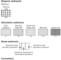
material is recorded on the barrel sheets (found in “Core Descriptions”) using symbols to represent up to three components in the Graphic Lithology col-umn (Fig. F2). Where an interval of sediment is a mixture of lithologic components, the constituent categories are separated by a solid vertical line, with each category represented by its own symbol. In con-trast, constituent categories separated by a dashed vertical line indicate intervals of thinly interbedded sediments comprising two or more lithologies of dif-ferent compositions. Constituents accounting for <10% of the sediment in a given lithology are not shown in the Graphic Lithology column but are listed in the Lithologic Description section of the core description form. Because of the limited scale of the core summaries, the Graphic Lithology column usually shows only the composition of layers or in-tervals exceeding 20 cm in thickness.

The Structure column indicates the presence of pri-mary sedimentary structures, soft-sediment modifi-cation features, structural features, and diagenetic features observed visually (Fig. F3). The following definitions were adopted from Blatt et al. (1980, p. 128):

• Thick bedding/color banding = beds/bands > 30 cm thick.

• Medium bedding/color banding = beds/bands 10– 30 cm thick.

• Thin bedding/color banding = beds/bands < 10 cm thick.

The following scale is used to describe bioturbation as measured by the percentage of burrow features: • Slightly bioturbated = 1%–30% bioturbation. • Moderately bioturbated = 30%–60% bioturbation. • Heavily bioturbated = 60%–90% bioturbation. Total mixing of sediment by bioturbating organisms produces homogeneous sediment with an appear-ance similar to nonbioturbated sediments that result from the deposition of material of homogeneous color and grain size. Therefore, a bioturbation scale cannot be applied to homogeneous sediment with confidence.

Deformation and disturbances of sediment that clearly resulted from the coring process are illus-trated in the Drilling Disturbances column of the barrel sheets (see “Core Descriptions”). The degree of drilling disturbance is described for soft and firm sediments using the categories listed below (blank re-gions indicate the absence of drilling disturbance): • Slightly disturbed = bedding contacts that are

(6)

• Moderately disturbed = bedding contacts that are extremely bowed or sediment biscuits that are rotated but likely still in stratigraphic order. • Very disturbed = bedding that is completely

dis-turbed or sediment biscuits that are likely rotated and no longer in stratigraphic order.

• Drilling slurry or flow-in = intervals that are water-saturated or have otherwise lost all aspects of original bedding resulting from flow-in or the presence of drilling slurry.

The degree of fracturing in indurated sediments is described in the Drilling Disturbance column using the following categories:

• Slightly fractured = core pieces that are in place and contain little drilling slurry or breccia.

• Moderately fragmented = core pieces that are in place or partly displaced, but the original orienta-tion is preserved or recognizable (drilling slurry may surround fragments).

• Highly fragmented = pieces that are from the cored interval and probably in the correct strati-graphic sequence (although they may not repre-sent the entire section), but the original orientation is completely lost.

• Drilling breccia = core pieces that are no longer in their original orientation or stratigraphic position and may have been mixed with drilling slurry. The hue and chroma attributes of color are recorded in the Color column of the barrel sheet and were de-termined using Munsell Soil Color Charts (1971). Figures summarizing key data from smear slides and XRD analyses appear in the “Sites M0001–M0004”

chapter.

The lithologic description that appears in the De-scription column of each barrel sheet lists all the ma-jor and minor sediment lithologies observed in the core, as well as a more detailed description of these sediments including features such as color, composi-tion (determined from the analysis of smear slides), or other notable characteristics. Descriptions and lo-cations of thin, interbedded, or minor lithologies or thin color banding that could not be depicted in the Graphic Lithology column are included in the text. Terms to describe sediment induration (e.g., firm) follow those used during ODP Leg 105 (Shipboard Scientific Party, 1987).

X-ray diffraction

Equipment parameter

X-ray diffraction (XRD) measurements were per-formed at the Crystallography Department of Geo-sciences, University of Bremen, on a Philips X’Pert

Pro X-ray diffractometer equipped with a Cu tube (Kα λ 1.541), a fixed divergence slit (¼°2θ), a 15-sample changer, a secondary monochromator, and the X’Celerator detector system. Measurements were made from 3° to 85°2θ with a calculated step size of 0.016°2θ. The calculated time per step was 100 s. Peak identification was done graphically through the Ma-cIntosh program MacDiff (version 4.5) (available at

servermac.geologie.uni-frankfurt.de/Staff/Home-pages/Petschick/RainerE.html) (Petschick et al., 1996).

Mineral identification

Integrated intensities for the investigated mineral peaks were calculated by MacDiff. Based on this in-tensity, ratios were calculated. To provide an easy comparison to published data on surface samples of the potential source regions (Andersen et al., 1996; Vogt, 1997; Vogt et al., 2001), the fixed divergence was changed to automatic divergence using an algo-rithm integrated in MacDiff.

Sediment classification

Expedition 302 sediment classification is based pri-marily on visual core descriptions and smear slide analyses. A modified version of the sediment classifi-cation format established during ODP Leg 151 (Ship-board Scientific Party, 1995) is used here to allow for easier comparison of the lithostratigraphy of cores retrieved during both cruises. As during Leg 151, the principal lithologic name (e.g., diatom ooze, silty clay) is based on the major (>50%) sediment compo-nent. Secondary components, composing 25% to 50% of the sediment, are included as major modifi-ers preceding the principal name (e.g., diatom ooze, silty clay). Minor constituents, composing 10% to 25% of the sediment, are included using the term “-bearing” (e.g., mud-bearing diatom ooze). The sed-iment modifiers are ordered so that minor modi-fier(s) precedes major modimodi-fier(s). Specific nomencla-ture for the two compositional groups, appropriate for sediments recovered during this expedition, is given below.

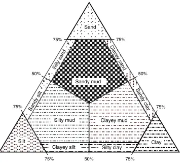
Siliciclastic sediments

(7)

modifier describing the secondary grain size. For ex-ample, siliciclastic sediment containing 70% clay and 30% silt would be classified as “silty clay.” In sit-uations where the siliciclastic sediment contains a mixture of sand, silt, and clay and the least abun-dant of these components comprises 10% of the sed-iment, the term “mud” is given as the major compo-nent and is modified by the name given to the most abundant grain size. For example, a mixture of 10% sand, 60% silt, and 30% clay would be classified as “silty mud.”

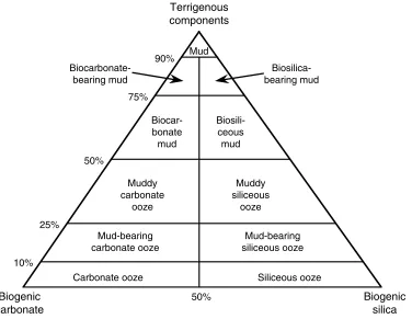
Biogenic sediments

The biogenic category includes fine-grained sedi-ments containing >50% biogenic sedisedi-ments. Desig-nation as siliceous or carbonate depends upon the relative abundance of these two biogenic categories (Fig. F5). When the biogenic component is >90%, the sediment is classified as ooze. When biogenic sediments are mixed with 10% to 25% siliciclastic components, the siliciclastic component name fol-lowed by the word “-bearing” is used as a major modifier. For example, if the sediment contains 80% biogenic silica of mixed types (e.g., diatoms, ebridi-ans, and silicoflagellates) and 20% siliciclastic clay, it would be classified as “clay-bearing biosiliceous ooze.” When the siliciclastic component is a mixture of sand, silt, and clay, the modifier “mud-bearing” is used (e.g., mud-bearing siliceous ooze).

Micropaleontology

Calcareous nannofossils

The zonal scheme of Martini (1971) was used for Cenozoic calcareous nannofossil biostratigraphy. This zonation represents a general framework for biostratigraphic classification of calcareous nanno-fossil assemblages. Many additional nannonanno-fossil bio-horizons are also used for dating and correlation. Nannofossil taxonomy follows that of Perch-Nielsen (1985a).

Calcareous nannofossils were examined on smear slides using standard light microscope techniques under cross-polarized and transmitted light at 1000× magnification. The following abbreviations were used to describe nannofossil preservation:

G = good (little or no evidence of dissolution and/or recrystallization; diagnostic charac-ters fully preserved).

M = moderate (dissolution and/or secondary overgrowth; partially altered primary mor-phological characteristics; most specimens were identifiable to the species level).

P = poor (severe dissolution, fragmentation, and/or overgrowth; primary morphological characteristics largely destroyed; specimens often could not be identified at the species and/or generic level).

Five calcareous nannofossil abundance levels are re-corded as follows:

A = abundant (>10 specimens observed/field of view [FOV]).

C = common (5–10 specimens observed/FOV). S = scarce (1–5 specimens observed/FOV). R = rare (<1 specimen observed/FOV). B = barren.

Diatoms

The Neogene Nordic Seas diatom zonation of Koç and Scherer (1996), the North Pacific diatom zona-tion of Akiba (1986), and the Neogene North Pacific diatom (NPD) zone code system of Yanagisawa and Akiba (1998) are used for the Neogene intervals. The Oligocene and Eocene zonation is modified from the Norwegian Sea diatom zonation of Schrader and Fenner (1976), Dzinoridze et al. (1978), Fenner (1985), and Scherer and Koç (1996). Absolute ages for diatom biostratigraphic horizons were updated from the Cande and Kent (1995) geomagnetic polar-ity timescale (GPTS).

Most slides were prepared as smear slides. However, strewn slides were prepared from the core catcher samples using the method of Akiba (1986) by placing a small amount of material in a snap-cap vial and re-moving part of the upper suspension with a pipette. The sample (~1 g) was placed in a 250 mL beaker, heated at 100°C for 1–2 h, and broken into pieces, af-ter which 100 mL of boiling distilled waaf-ter was added. After the distilled sample soaked for 6 h, the supernatant fluid was skimmed. Additional distilled water was then added to obtain a solution of suitable density. The solution was left for 30 s to let grains denser than diatoms, such as grains of quartz, settle to the bottom of the beaker. Strewn slides were pre-pared by spreading the pipette suspension on a cov-erslip (22 mm × 30 mm), drying on a hot plate (50°– 60°C), and mounting in Pleurax.

(8)

valves were observed for samples containing suffi-cient diatom remains. When fewer than 200 diatom valves were encountered on a slide, all taxa were enumerated in a single count.

Except for the core catcher samples, assessment of total diatom abundance was qualitative. Diatoms were recorded as follows:

A = abundant (≥6 specimens/FOV. C = common (1–5 specimens/FOV). F = few (1–4 specimens/5 FOV).

R = rare (1–10 specimens/horizontal traverse). Diatom preservation categories reported in the range charts are described according to Koç and Scherer (1996) as follows:

G = good (finely silicified and robust forms present; no significant alternation of the frustules other than moderate fragmenta-tion).

M = moderate (concentration of more heavily si-licified forms and/or a high degree of frag-mentation of finely silicified forms).

P = poor (finely silicified forms virtually absent; heavily silicified forms fragmented and/or corroded).

Silicoflagellates

Prior to Expedition 302, silicoflagellates had not been observed in any sediment from the Lomonosov Ridge. Previous silicoflagellate studies from neighbor-ing regions, however, includneighbor-ing the Alpha Ridge in the Arctic Ocean, were used for reference. Based on the sediments recovered during Leg 151 from the Fram Strait and the Norwegian-Greenland Sea, a bio-stratigraphic zonal scheme has been established for the early Eocene through the Quaternary (Locker, 1996). Amigo (1999) worked on ODP Leg 162 materi-als from the Iceland and Rockall plateaus, and pro-posed new Miocene silicoflagellate zones. Perch-Nielsen (1985b) compiled comprehensive references on silicoflagellate biostratigraphy from the World Ocean. Silicoflagellates and ebridians were reported from the Alpha Ridge in Core FL-422 (Bukry, 1984; Ling, 1985; Dell’Agnese and Clark, 1994). Estimated ages were all adjusted to the GPTS for Expedition 302. Core catcher samples were disaggregated and decalci-fied by gentle boiling in a solution of 10% H2O2 and

10% HCl for ~2 h. A solution of Calgon was added to the sample solution and thoroughly stirred to fur-ther disaggregate the sediments and raise the pH level. Distilled water was repeatedly added to neu-tralize the sample solution before sieving through a 45 µm stainless steel screen. Smear slides of both the coarse fraction (>45 µm) and the fine fraction (<45 µm) were prepared by pipetting the sediments onto

glass slides. The water was allowed to evaporate, and a drop of xylene was added to purge the sediments of remaining water. Finally, Canada balsam was added to the slide, and a 22 mm × 50 mm coverslip was placed on top. The coarse fraction was primarily used for the study of silicoflagellates, although the fine fraction was also investigated to account for smaller-sized specimens (<45 µm).

Total silicoflagellate and ebridian abundances were determined along eight traverses (perpendicular to the length of slide) at 400× magnification, using the following convention:

A = abundant (>50 specimens). C = common (16–50 specimens). F = few (3–15 specimens). R = rare (2–3 specimens). T = trace (1 specimen). B = barren (none on a slide).

Preservation of silicoflagellates and ebridians was re-corded as follows:

G = good (majority of specimens complete, with minor dissolution and/or breakage).

M = moderate (minor but common dissolution, with a small amount of specimen breakage). P = poor (strong dissolution and/or breakage;

many specimens unidentifiable).

Radiolarians

No radiolarian biostratigraphic zonation has been developed for the Arctic Ocean. However, a biostrati-graphic scheme for the Norwegian Sea (e.g., ODP Leg 104, Goll and Bjørklund, 1989) extends back to near the base of the Miocene and contains 30 zones. It builds upon the study carried out during DSDP Leg 38 by Bjørklund (1976), which includes eight zones covering the Oligocene and Eocene. The radiolarian biostratigraphy used for Expedition 302 is based largely on these two radiolarian zonations. Other high-latitude zonations have been developed for the North Pacific Ocean (e.g., Kamikuri et al., 2004), but it is uncertain how applicable these zonations will be in the Arctic Ocean.

Samples were disaggregated by heating in a solution of 10% H2O2. Calcareous components were then

(9)

some Canada balsam, and covering with a 22 mm × 40 mm glass coverslip. Alternatively, after drying, the glass coverslips were mounted using 8–12 drops of Norland optical adhesive 61.

Total radiolarian abundances were determined based on strewn slide evaluation at 100× magnification, us-ing the followus-ing convention:

A = abundant (>100 specimens/slide traverse). C = common (51–100 specimens/slide traverse). F = few (11–50 specimens/slide traverse). R = rare (1–10 specimens/slide traverse). T = trace (<1 specimen/slide traverse). B = barren (no radiolarians in sample).

Individual species abundances were recorded relative to the fraction of the total assemblages as follows:

C = common (>2000 specimens/slide). F = few (200–2000 specimens/slide). R = rare (20–200 specimens/slide). VR = very rare (2–20 specimens/slide). + = trace (<2 specimens/slide).

B = barren (no radiolarians in sample). Preservation was recorded as follows:

G = good (majority of specimens complete, with minor dissolution, recrystallization, and/or breakage).

M = moderate (minor but common dissolution, with a small amount of specimen breakage). P = poor (strong dissolution, recrystallization, or breakage; many specimens unidentifiable).

Foraminifers

Preparation methods used to obtain calcareous, ag-glutinated, and planktonic foraminifers include dis-aggregation and wet-sieving over a 63 µm sieve. The sieved residues were dried, and the foraminifers were separated from the sand fraction under a binocular microscope. Several methods were used to disaggre-gate the sediment sample, including boiling in hot Calgon solution. The volume of original core catcher sample was variable, but ~10–20 cm3_{was processed}

whenever possible. Abundances of the foraminifers per ~10–20 cm3_{sample are characterized as follows:}

A = abundant (>250 specimens). C = common (25–250 specimens). F = few (5–25 specimens).

R = rare (1–5 specimens).

B = barren (no foraminifers in sample).

Calcareous benthic foraminifers

Calcareous benthic foraminifers have been studied from Legs 104 and 151 (Osterman and Qvale, 1989; Osterman and Spiegler, 1996; Osterman, 1996). Shal-low-water, high-latitude benthic foraminifers from

Baffin Island, Greenland, and the North Sea have been extensively studied by Feyling-Hanssen and colleagues (e.g., Feyling-Hanssen et al., 1983; Fey-ling-Hanssen, 1990; Knudsen and Asbjørnsdottir, 1991). Quaternary calcareous foraminifers from cen-tral Arctic Ocean deep-sea cores have been studied by Scott et al. (1989), Ishman et al. (1996), and Polyak et al. (2004). Taken together, calcareous benthic fora-minifers provide a means to correlate Pleistocene sediments from the central Arctic Ocean with those from adjacent regions.

Agglutinated benthic foraminifers

No formal zonal scheme for agglutinated foramini-fers yet exists for the Cenozoic of the central Arctic Ocean, as these microfossils have only been studied from comparatively short piston cores that recovered the last few glacial cycles (Evans and Kaminski, 1998). Fortunately, however, regional zonations have been set up for several areas along the circum-Arctic shelves, including the Cenozoic of the Beaufort Sea– MacKenzie Delta region (Schröder-Adams and Mc-Neil, 1994; McMc-Neil, 1997), the Paleogene of the Western Barents Sea (Nagy et al., 2000, 2004), and the Paleogene of the western Siberian lowlands (Podobina, 1998). Studies of ODP sites in the Norwe-gian-Greenland Sea provide a basis for establishing the taxonomical affinities of Arctic foraminifers with localities farther south. Miocene biostratigraphy at ODP Site 909 in Fram Strait was established by Oster-man and Spiegler (1996); Kaminski and Austin (1999) studied the Oligocene at ODP Site 985 on the Iceland Plateau. The Eocene foraminiferal record is known from ODP Site 643 on the Vøring slope (Ka-minski et al., 1990). The Cenozoic biostratigraphic record (mostly Paleocene to Miocene) of the North Sea and Labrador Sea was established by Gradstein et al. (1994). The stratigraphic record of agglutinated foraminifers in the Norwegian Sea area is continuous from the early Paleocene to the late Miocene, and with well over a hundred taxa reported from the area, this group provides good potential for strati-graphic correlation.

Planktonic foraminifers

The standard low-latitude biostratigraphic zonation of Berggren et al. (1995) is not applicable to the Arc-tic region; therefore, direct correlations of plank-tonic foraminifers to the GPTS is not possible. In-stead, comparisons were made with the regional biostratigraphy established at ODP sites in the Nor-wegian-Greenland Sea (Spiegler and Jansen, 1989; Spiegler, 1996) that make use of local planktonic for-aminiferal first and last occurrences, coiling changes

(10)

zona-tion of Weaver and Clement (1986). Unfortunately, the pre-Pliocene record of planktonic foraminifers in the Norwegian-Greenland Sea area is patchy at best and no biostratigraphic zonation exists for the area.

Ostracodes

There is no formal biostratigraphic zonation for Cen-ozoic ostracodes from the Arctic Ocean; however, there are stratigraphic range data for many species found in widely scattered literature. Prior ODP legs have yielded preliminary information on Neogene ostracodes from the Vøring Plateau (Malz, 1989; Leg 104 Sites 642–644) and the Yermak Plateau (Cronin and Whatley, 1996; Leg 151 Sites 910 and 911). Both studies were of a preliminary nature, and no formal ostracode zonation was developed.

Outcrop exposures and shallow-water cores from the circum-Arctic and sub-Arctic regions in the North At-lantic and Pacific regions provide additional strati-graphic information on high-latitude northern hemisphere species (see Cronin et al., 1993, for a re-view). These studies include the Pliocene of the Alaska Coastal Plain (Repenning et al., 1987), the Pliocene–Pleistocene Iperk sequence in the eastern Beaufort Sea (Siddiqui, 1988), the Pliocene Kap Kobenhaven and Lodin Elv formations of Greenland (Brouwers et al., 1991; Penney, 1990, 1993), the Tjornes, Iceland, Pliocene–Pleistocene (Cronin, 1991), and Paleocene of West Greenland (Szcze-chura, 1971).

Shallow-water ostracode zonations for the Cenozoic of the British Isles (Keen, 1978), France (Oertli, 1985), and Germany and the Cenozoic of the deep North Atlantic (Coles and Whatley, 1989; Whatley and Coles, 1987) will also be useful in correlating Ex-pedition 302 cores with other regions.

Previous coring in the deep Arctic Ocean has yielded abundant data on ostracodes from the last few gla-cial and interglagla-cial cycles of the Quaternary (Cronin et al., 1994, 1995; Polyak et al., 2004). These studies show that ostracodes are highly sensitive to oceano-graphic changes related to Arctic water mass and sea-ice conditions.

Ostracodes were picked from the >150 µm size frac-tion of the micropaleontological residue used for for-aminiferal studies.

The following categories were used to describe ostra-code abundance:

A = abundant (>250 specimens). C = common (25–250 specimens). F = few (5–25 specimens).

R = rare (1–5 specimens).

B = barren (no specimen present).

Palynology, organic-walled

dinoflagellate cysts

In the absence of an established zonation scheme for the Arctic Ocean, the distribution pattern of index taxa is compared to the global Late Cretaceous–Cen-ozoic compilation of Williams et al. (2004). In addi-tion, comparisons were made to relevant northern high-latitude studies, including those of Head and Norris (1989), Firth (1996), Williams and Manum (1999), and Eldrett et al. (2004).

Samples were processed on board using sodium hexametaphosphate, following the procedures de-scribed by Riding and Kyffin-Hughes (2004). “Heavy-liquid” (ZnCl2) separation was applied. Following

sieving over a 20 µm sieve, strewn mounts of the res-idue were made using glycerine jelly. Organic-walled dinoflagellate cysts (dinocysts) were counted to >100 specimens, whereas other major categories of pa-lynomorphs (e.g., bisaccate pollen, spores, and fora-minifer linings) were also taken into account. Di-nocyst taxonomy is in accordance with that cited in Williams et al. (1998).

Fish teeth

Although fish teeth have been used for biostratigra-phy in the Pacific Ocean (e.g., Doyle and Riedel, 1979), we extracted ichthyoliths from the sediment primarily for the purpose of making geochemical measurements (e.g., Gleason et al., 2004, and refer-ences therein). Samples (20 cm3_{) of raw sediment}

were disaggregated and sieved using only distilled water. Individual fish teeth were picked from the coarse residue and stored in a cardboard slide for each sample. These specimens were then further chemically cleaned prior to analysis according to the procedure of Gleason et al. (2004). The presence of other fossil fish material in Hole M0004A is shown in the foraminiferal occurrence table.

Stratigraphic correlation

Composite depths

(11)

Several aspects of Expedition 302 necessitate a modi-fied approach toward hole-to-hole stratigraphic cor-relation and generation of composite depths com-pared to previous, non-MSP cruises. In particular, the shorter core length (~4.5 m at full recovery, com-pared to ~9.5 m with IODP) and a limited number of planned holes (two to three) make it more challeng-ing to ensure complete overlap of cores. Durchalleng-ing Ex-pedition 302, the main mode of stratigraphic corre-lation was actually a site-to-site correcorre-lation, as the drill sites are close to each other and are tied to-gether confidently by seismic stratigraphy.

The offset in depth required in subsequent holes must rapidly be determined before and during cor-ing. The continuity of recovery is assessed by devel-oping composite sections that align prominent fea-tures in physical property data from adjacent holes. The procedure and rationale for this stratigraphic correlation is described in this section and follows the methodology pioneered during ODP Legs 94 (Ruddiman et al., 1987) and 138 (Hagelberg et al., 1992). Similar methods were employed and devel-oped further during ODP Legs 154 (Curry, Shackle-ton, Richter, et al., 1995), 162 (Jansen, Raymo, Blum, et al., 1996), 167 (Lyle, Koizumi, Richter, et al., 1997), 171B (Norris, Kroon, Klaus, et al., 1999), and more recent ODP legs such as 199 (Shipboard Scien-tific Party, 2002; Pälike et al., 2005). During ODP Leg 202 it was found that vertical tidal movements can have a significant impact on the predicted meters be-low seafloor depth for a given stratigraphic interval (Shipboard Scientific Party, 2003). For Expedition 302, tidal movements were expected to be small, and this was confirmed precruise for the anticipated drill-ing days and locations, with predicted tides of less than a few tens of centimeters (L. Erofeeva, pers. comm., 2004; Padman and Erofeeva, 2004).

Data employed for stratigraphic correlation

Onboard stratigraphic correlation requires closely spaced data that can be generated rapidly. After each whole-core section had equilibrated to room temper-ature (typically 3–5 h), it was run through the cus-tom-modified Geotek MSCL (see “Petrophysics”). The MSCL generates high-resolution (down to 2 cm intervals) measurements of magnetic susceptibility (MS), gamma ray attenuation (GRA) bulk density, P -wave velocity, and electrical resistivity (RES). Natural gamma radiation (NGR) and color reflectance data were not measured during the offshore phase and were instead measured during the onshore phase at BCR.

The MSCL was run in two separate modes: rapid and standard. In the rapid mode, the MSCL was run

us-ing two MS loops at a depth resolution of 2 cm; other parameters were measured at a depth resolu-tion of 4 cm. The cores were measured quickly after retrieval, and their temperature may not have neces-sarily equilibrated with the laboratory temperature. Thus, the data are not absolute values of MS and were only used for initial offshore stratigraphic cor-relation. In the standard mode, all MSCL parameters (MS, bulk density, P-wave velocity, and RES) were measured at a depth resolution of 2 cm. As the core flow was lower than expected, both MS loops were used to measure susceptibility values at the same po-sitions downcore. These duplicate measurements were used for quality control and were averaged where appropriate. The data files saved from the Geotek (version 7.3) software (both raw and pro-cessed) were copied across to a dedicated strati-graphic correlation computer via the network, where data from individual cores were assembled into a continuous downhole record with custom written conversion scripts. These scripts also attached mbsf depths for each measurement, as the output from the Geotek software is limited to downcore depths. For the detailed setup of the Geotek scanner, see

“Petrophysics.” During the coring operation, it be-came clear that geochemical data could be used for stratigraphic correlation purposes. Ammonia con-centrations (see “Geochemistry”) were loaded into the stratigraphic correlation software and comple-mented the stratigraphic correlation process.

During the onshore phase, cores were run through an MSCL with an NGR emission sensor. NGR data were generated at 6 cm intervals and proved useful in the correlation of cores, with a distinct signal throughout the stratigraphic intervals recovered. In addition, measurements of color reflectance in the 400–700 nm wavelength range and calculated L*a*b* values were made at a 5 cm depth resolution on the split archive half of the core using a Minolta spectro-photometer (see “Petrophysics”). The red-green parameter (a*), in particular, proved useful for corre-lation of distinct color changes between the litholo-gies.

(12)

Composite section development

IODP sample and core depths are recorded in mbsf from the first core in each hole that shows a true mudline, and consecutive depth measurements are determined by the length of the drill string. Several factors can lead to a deviation of the relative distance of geological features in the core from their true in situ stratigraphic separation. For example, sediment inside the core can expand as a result of reduced ef-fective stress following core recovery, leading to an expanded sedimentary sequence relative to its origi-nal length (Moran, 1997). Thus, sediment can be missing between cores, even if a nominal 100% re-covery is achieved. In addition, variations in ship motion, tides, and heave can result in stretching and/or squeezing of the recovered sediment in par-ticular intervals and even multiple recovery of iden-tical stratigraphic intervals in consecutive cores. To allow the placement of geological data from different holes according to their stratigraphic position, phys-ical property measurements are correlated to create a meters composite depth (mcd) scale. The generation of a mcd scale attempts to match coeval stratigraphic features, as recorded by the MSCL and color reflec-tance measurements, at the same level by generating a composite record from different holes. This process requires depth shifting cores relative to each other. During this step, the total length on the mcd scale is typically expanded by 10% compared to the mbsf scale, although this factor can vary between ~5% and 15% (Hagelberg et al., 1992; Norris, Kroon, Klaus, et al., 1998). Site-to-site and hole-to-hole cor-relation was facilitated by using the graphical and in-teractive UNIX platform software, Splicer (version 2.2), which was developed by Peter deMenocal and Ann Esmay of the Lamont-Doherty Earth Observa-tory Borehole Research Group (LDEO-BRG) (avail-able on the World Wide Web at www.ldeo.colum-bia.edu/BRG/ODP). Significant modifications were made for this expedition (by H. Pälike) to run the program on Mac OSX 10.3. The log-integration soft-ware Sagan was also modified.

Splicer allows data sets from adjacent holes to be cor-related simultaneously, making use of interactive cross-correlation computation. After prominent fea-tures are aligned and referenced to a new mcd scale, a spliced record is generated by switching holes to avoid core gaps or disturbed sediment, resulting in a continuous record. Another output of the composite depth scale is generation of a template that forms the basis for sediment sampling along a complete section, thus minimizing duplicate sampling and saving analytical time. For this reason, it is highly desirable to apply a constant offset to an entire core such that the depth increments along individual

cores on the mcd scale are linearly related to the cu-rated core depth increments. Splicer only allows the application of a constant offset for each core. How-ever, composite depth scales created using the Splicer method are usually not satisfactory to create a stacked record from different holes because not ev-ery individual feature present across different holes can be aligned. Hence, if the aim is to increase the signal-to-noise ratio of quasi-periodic cycles that might be recorded in the sedimentary record, it is important to allow stretching and squeezing within individual sections so that data from different holes on the individual cycle level are aligned.

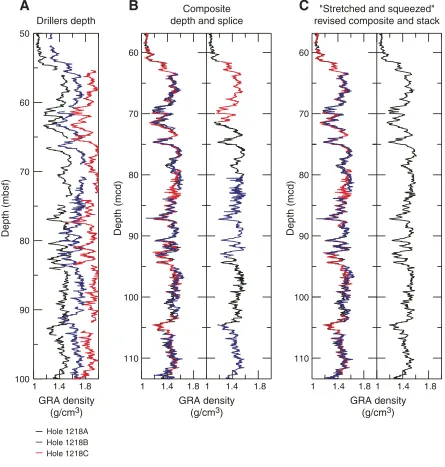
The procedure for generating a common depth scale that allows stretching and squeezing on a fine level was pioneered by Hagelberg et al. (1995) and results in a revised mcd (rmcd) common depth scale. Gener-ation of rmcd scales is typically conducted as part of postcruise work. Composite depth generation using Splicer first begins by assigning the core with the best record of the upper few meters of a hole as the top of the composite record, and it typically contains the mudline. This core is assigned an mcd identical to its mbsf depth. A tie point, which gives the pre-ferred correlation, is selected between data from this first core and a core in a second hole. All the data from the second hole below the correlation point are vertically shifted to align the tie points between the holes. After choosing an appropriate tie point and adjusting the depths, the shifted section becomes the next “reference” section and a tie is made to a core from the first hole. Working downhole in an it-erative fashion, each core is then vertically shifted. Where there is no overlap, consecutive cores are ap-pended. The tie points are recorded in a Splicer out-put (“affine”) table in units of mcd. The affine table that relates mbsf to mcd values along with the ap-plied linear offsets for each core is presented in tabu-lar form in “Stratigraphic correlation” in the “Sites M0001–M0004” chapter. A shortened composite depth table for Site M0004 is given as an example in Table T3. The last two columns in each table give, for each core, the cumulative depth offset added to the IODP curatorial subbottom depth (in mbsf) and the composite depth (in mcd), respectively. The depth offset column allows the calculation of the equiva-lent depth in mcd by adding the amount of offset listed to the depth in mbsf of a sample taken in a particular core. Table T4 shows a typical example for the Splicer file that defines the switching across holes to generate a spliced composite section. The composite depth and splice-tie point tables from each site chapter are also available in ASCII.

(13)

features (example from Leg 199, Site 1218; Pälike et al., 2005). In the left panel, MS data from three holes at one site are shown on the mbsf depth scale, whereas in the middle panel, the data are shown on a common depth (mcd) scale together with a gener-ated spliced record, indicating where the sample track was switched from one hole to the next. The right panel shows the rmcd scale, where individual physical property features were aligned by stretching and squeezing, together with a final stacked record from all holes. If the available data allow only an ambiguous or imprecise correlation or if multiple hole data were unavailable, no additional depth ad-justments were made. In this case, the cumulative offset remains constant for all subsequent cores. On several occasions cores had a recovery >100% per-cent, resulting in overlapping mbsf depths. For these cores, we applied small vertical offsets to avoid over-lap, while generally trying to keep mcd values close or identical to mbsf depths where there was no over-lap between holes. Splice tie points were made be-tween adjacent holes at identifiable, highly corre-lated features and were placed at transitions rather than peaks. Each splice was constructed beginning at the mudline at the top of the composite section and worked downward. Typically, one chooses one hole as the backbone for the record and cores from other holes are then used to patch in the missing intervals in core gaps (Fig. F6). Intervals were chosen for the splice such that section continuity was maintained, whereas disturbed intervals were avoided. The final alignment of the adjacent holes could be slightly dif-ferent from the best overall visual or quantitative hole-to-hole correlation because of the constraint that a constant offset be applied to each core by the Splicer software.

Technological advancements

During Expedition 302, it was important to use the stratigraphic correlation to make coring decisions in near real time. This was achieved by introducing sev-eral modifications to the standard IODP protocol. Crossover between shifts was done over the Internet connection (mirroring the correlation computer screen between ships). Stratigraphic correlators were able to view the status of the splice on computers while they talked by mobile telephone between the drilling vessel Vidar Viking and the operations center vessel Oden.

In addition to the MSCL data, lower-resolution core catcher sample data (age, grain size, color, and den-sity) were used to support this work. Scientists aboard Oden provided these supplemental data by regularly updating an Excel spreadsheet with this in-formation on the central server, which was available

across vessels by means of wireless data transfer and networking. A faster throughput of cores through the MSCL was achieved by incorporating two MS loops calibrated and run at slightly different frequen-cies.

Petrophysics

The primary objective of the petrophysical program was to collect high-resolution data to

1. Allow hole-to-hole correlation and facilitate the retrieval and construction of a complete compos-ite stratigraphic section,

2. Provide data for construction of synthetic seismo-grams to allow near-real-time tracking of drilling progress and to investigate the characteristics of major seismic reflectors, and

3. Provide data for characterization of lithologic units.

Petrophysical measurements were either performed on whole cores and discrete samples or were made in situ through wireline logging or specialized down-hole tools. The bulk of the petrophysical program was associated with collecting high-resolution, non-destructive measurements on whole cores using the Geotek MSCL. While offshore, the MSCL was outfit-ted with four sensor types capable of measuring bulk density, MS, transverse compressional wave (P-wave) velocity, and RES (see “Stratigraphic correlation”). The MSCL was used onshore to acquire digital line scan images, measure P-wave velocity on selected sections where whole-core measurements performed offshore resulted in poor quality data, and measure bulk density and MS on one core (302-M0004C-6X) that was too thick to fit through the MS loops off-shore.

Lower-resolution MAD, shear strength, color reflec-tance, and needle-probe thermal conductivity mea-surements were also routinely performed. A helium gas pycnometer was used to measure the volume (for density determinations) of discrete samples taken from the core catchers of each core while offshore and at an approximate resolution of one per section from the working half of split cores at BCR. This al-lowed an independent determination of bulk den-sity, grain denden-sity, water content, poroden-sity, and void ratio, which were used to calibrate the high-resolu-tion, nondestructive measurements made with the MSCL.

In situ temperature measurements were made with two different tools, the Adara tool (from ODP) and a BGS-supplied tool.

(14)

The tool string measured microresistivity using the Formation MicroScanner (FMS), P-wave velocity us-ing the Borehole Compensated Sonic (BHC) tool, to-tal NGR emissions using the Scintillation Gamma Ray Tool (SGT), and spectral emissions using the Natural Gamma Ray Spectrometry Tool (NGT).

MSCL measurements

The principal aim of MSCL data acquisition during the offshore component of Expedition 302 was to obtain high depth-resolution data sets to facilitate shipboard core-to-core correlation during construc-tion of composite stratigraphic secconstruc-tions. The MSCL was run in two separate modes: rapid and standard. In rapid mode, the MSCL could be run using two MS loops, both set at a resolution of 4 cm. Because the loops would measure out of sequence with one an-other, the resulting MS data had a downcore resolu-tion of 2 cm. In rapid mode, cores were run quickly and were not necessarily equilibrated to laboratory temperature. In standard mode, both MS loops per-formed susceptibility measurements in conjunction with GRA density, P-wave velocity, and resistivity measurements. Standard resolution for all instru-ments was 2 cm. Standard mode measureinstru-ments were performed on temperature-equilibrated cores. Cores that were to be sampled for geochemistry and micro-biology were all logged in rapid mode prior to re-moving whole rounds, samples, or pore water (see

“Geochemistry”). Sampled cores were subsequently logged in standard mode, and correlation between rapid and standard modes will be used to correct the rapid-logged data if deemed necessary. All MSCL data included in the this volume are from standard-mode logging.

MSCL measurement principles

Magnetic susceptibility

Whole-core MS was measured with the MSCL using two Bartington MS2 meters and MS2C loop sensors. The MS2C loop sensors had an internal diameter of 80 mm, which corresponds to a coil diameter of 88 mm. It normally operates at a frequency of 0.565 kHz and an alternating-field (AF) intensity of 80 A/m (= 0.1 mT). During the offshore component of Expe-dition 302, two Bartington loops were installed on the MSCL to enable rapid core logging. The necessity for rapid logging originated from the need to have near real-time stratigraphic correlations to help guide drilling decisions. In order to have two sensors operating concurrently without interference, their operating frequencies were offset. MS1 was set to an operating frequency of 621 Hz, and MS2 was set at 513 Hz. Correction factors for each of the sensors (1.099× for MS1 and 0.908× for MS2) were used to

adjust the values equivalent to measurement at the standard 565 Hz. Calibration standards with bulk susceptibility (χ) of 210 × 10–6_{cgs (MS1) and 213}×

10–6_{cgs (MS2) were used to check the operation of}

each susceptibility sensor. The MSCL software auto-matically corrected the MS data for the dual operat-ing frequencies in the processed data output.

The MS2C meter operates on two sensitivity levels, 0.1× and 1×, which correspond to a 10 s and 1 s sam-pling period, respectively. The higher sensitivity set-ting results in measurements to the first decimal place, with the 10-fold increase in measurement time providing additional noise filtering. The resolu-tion of the loop is 2 × 10–6_{SI on the 0.1 range (10 s}

measuring time). The effective sensor length of the 80 mm MS2C loop is 4 cm. During offshore Expedi-tion 302, MS measurements were routinely made at a spacing of 2 cm, with a single data acquisition made on the 1× range. MS data were archived as raw in-strument units and were not corrected for changes in sediment volume.

Density

Bulk density is estimated by measuring the attenua-tion of gamma rays that have passed through the cores, with the degree of attenuation being propor-tional to density (Boyce, 1976). Calibration of the system was completed using known seawater/alumi-num density standards (see Blum, 1997). Bulk den-sity data are of highest quality when determined on APC cores because the liner is generally completely filled with sediment. In XCB cores, density measure-ments are of lower quality and cannot necessarily be used to reliably determine bulk density on their own. The measurement length of the GRA sensor is ~0.5 cm, with sample spacing set at 2 cm during off-shore Expedition 302. The minimum integration time for a statistically significant GRA measurement is 1 s; routine GRA measurements were run at a 4 s integration time.

P-wave velocity

(15)

filled with distilled water were used to calibrate the offsets in traveltime that occur through the system components and core liner. The measurement width of the PWL sensor is ~0.1 cm, with sample spacing routinely set at 2 cm for Expedition 302 measurements.

Electrical resistivity

Electrical RES of sediment cores was measured using the noncontact resistivity (NCR) sensor on the MSCL. NCR measurements are made using a high-frequency magnetic field to induce an electrical cur-rent in the core. Magnetic fields, generated by the in-duced electrical current, are measured on a receiver coil and normalized with a third set of coils operat-ing in air. The NCR is calibrated by measuroperat-ing the re-sistivity of five standard 0.45 m core liner sections containing water of varying but known salinity and relating the known resistivity of each stock solution with the millivolt output from the meter. Standards were made by mixing a 7 L stock solution of 35,000 ppm NaCl distilled water. Dilution of the stock solu-tion allowed five standards to be made with concen-trations of 35,000, 17,500, 3,500, 1,750 and 350 ppm. By measuring the standards on the MSCL, an exponential regression was fit between resistivity (ohm-meters) and sensor output in millivolts. Values from the regression were entered into the MSCL soft-ware and applied internally to the raw sensor read-ings.

Natural gamma radiation

NGR emissions of sediments are a function of the random and discrete decay of radioactive isotopes, predominantly those of 238_U,232_{Th, and}40_{K, and are}

measured through scintillation detectors housed in a shielded collector. For the onshore phase of Expedi-tion 302, a Geotek frame system was employed that allowed up to six cores to be logged during a single run. The gamma ray detector has a measurement window of 7.5 cm, and the sampling interval was set at 6 cm, in order to maximize the resolution of mea-surements while minimizing resampling of intervals. The count time at each sampling point was set at 4 min. This sampling interval and count time pro-vided the highest resolution and best data quality possible within the time available to complete the core logging. The increased counting times required whole-core gamma ray logging to start 2 weeks prior to the arrival of the science party in Bremen, being completed at the end of the first week of the onshore phase. The data are presented as total counts per sec-ond and refer to the integration of all emission counts over the gamma ray energy range between 0 and 3 MeV and is best suited for core-to-core correla-tion. No corrections were made to NGR data to

ac-count for volume effects related to sediment incom-pletely filling the core liner.

Digital color imaging system

While onshore, systematic high-resolution line-scan digital core images of the archive half of each core were obtained using the Geotek X-Y digital imaging system (Geoscan II). This system collects digital im-ages with three line-scan charge-coupled device ar-rays (1024 pixels each) behind an interference filter to create three channels (red, green, and blue [RGB]). The image resolution is dependent on the height of the camera and width of the core. The standard con-figuration for the Geoscan II produces 300 dots per inch (dpi) on an 8 cm wide core, with a zoom capa-bility up to 1200 dpi on a 2 cm wide core. Synchro-nization and track control are better than 0.02 mm. The dynamic range is 8 bits for all three channels. The framestore card has 48 MB of onboard random access memory (RAM) for acquisition of images with an ISA interface card for personal computers. The system was calibrated at the start of each day. Output from the digital imaging system includes a Windows bitmap (.BMP) file and a compressed (.JPEG) file. The bitmap file contains the original data with no com-pressional algorithms applied. All cores were imaged using an aperture setting of f/5.6 except Cores 302-M0002A-52X and below in Hole M0002A (imaged using both f/5.6 and f/4) and Cores 302-M0004A-6X and below in Hole M0004A, which were imaged us-ing f/4. RGB curves were produced for undisturbed core sections by averaging across a 2 cm wide strip (4.5–6.5 cm) at an interval of 2 mm downcore. When utilizing the RGB data it is recommended that detailed examination of core photographs/images and disturbance descriptions/tables is undertaken in order to cull unnecessary or spurious data.

Diffuse color reflectance

spectrophotometry

Archive halves were measured at 5 cm intervals using a handheld Minolta spectrophotometer (model CM-2600d). Black and white calibration of the spectro-photometer was performed every 24 h. Prior to mea-surement, the core surface was scraped and covered with a clear plastic wrap to maintain a clean spec-trometer window.

(16)

Measurements were not performed on severely dis-turbed intervals, particularly in regions containing slurry and flow-in. Measurements on cores with bis-cuiting and rough surfaces slightly biased the digital and spectrophotometric data toward darker values. When utilizing the spectrophotometric measure-ments it is recommend that detailed examination of core photos/images and disturbance descriptions/ tables is undertaken in order to cull unnecessary or spurious data.

Moisture and density

MAD (bulk density, grain density, water content, po-rosity, and void ratio) was determined from measure-ments of wet and dry sediment mass and dry sedi-ment volume. Offshore, constant-volume samples of ~4.56 cm3_{were taken from core catchers that were}

brought aboard the Oden from the Vidar Viking. In general, one MAD sample from each core catcher was taken. Discrete samples were also taken from the working half of split cores at BCR. Onshore MAD sampling was at a resolution of ~1 per section. Sample mass was determined using the marine ana-lytical balance and associated Core Logic software. The balance was equipped with a computer averag-ing system that corrected for ship acceleration. The sample mass was counterbalanced by a known mass so that the mass differential was generally <1 g. After drying the sediment samples at 105°C for 24 h and weighing to determine the dry sediment mass, the samples were crushed using a mill grinder. Subsam-ples of ~3.6 cm3_{from the crushed sediment were}

weighed and prepared to determine volume using Micrometrics Accupyc 1330 pycnometer, a helium-displacement pycnometer capable of measuring one sample per run. The volume measurements were re-peated five times by the pycnometer software until the last two measurements exhibited <0.01% stan-dard deviation. A reference volume consisting of a 36.0604 g tungsten sphere was used on several occa-sions to check the instrument for drift and system-atic errors.

Onshore, discrete samples were extracted from the working half of split cores (~1 per section) and placed in 10 mL beakers where core recovery al-lowed. Sample mass was determined to a precision of 0.001 g using an electronic balance. Sample volumes were determined using a Quantachrome penta-pyc-nometer (helium-displacement pycpenta-pyc-nometer) with a precision of 0.02 cm3_{. Volume measurements were}

repeated a maximum of five times, or until the last three measurements exhibited <0.01% standard de-viation. A reference volume was included within each sample set and rotated sequentially among the cells to check for instrument drift and systematic

er-ror. A purge time of 1 min was used before each run. Dry mass and volume were measured after samples were heated in an oven at 105° ± 5°C for 24 h and al-lowed to cool in a desiccator. The procedures for de-termination of MAD are described in the offshore phase of the methods above and are not repeated here. The procedures for determination of MAD comply with the American Society for Testing and Materials (ASTM) designation (D) 2216 (ASTM, 2005).

Wet mass (Mwet), dry mass (Mdry), and dry volume

(Vdry) were measured in the laboratory. Salt

precipi-tated in sediment pores during the drying process is included in the Mdry and Vdry values. The mass of the

evaporated water (Mwater) and the salt (Msalt) in the

sample are given by

Mwater = Mwet – Mdry and

Msalt = Mwater [s/(1 – s)],

where s = assumed seawater salinity (0.035) and cor-responds to a pore water density (ρpw) of 1.024 g/cm3

and a salt density (ρsalt) of 2.257 g/cm3. The corrected

mass of pore water (Mpw), volume of pore water (Vpw),

mass of solids excluding salt (Msolid), volume of salt

(Vsalt), volume of solids excluding salt (Vsolid), and wet