A Forward Regression Algorithm based on M-estimators
Xia Hong
Department of Cybernetics
University of Reading
Reading, RG6 6AY, UK
[email protected]
Sheng Chen
School of Electronics and Computer Science
University of Southampton
Southampton, SO17 1BJ, UK
[email protected]
Abstract
This paper introduces an orthogonal forward regression (OFR) model structure selection algorithm based on the M-estimators. The basic idea of the proposed approach is to incorporate an IRLS inner loop into the modified Gram-Schmidt procedure. In this manner the OFR algorithm is extended to bad data conditions with improved performance due to M-estimators’ inherent robustness to outliers. An il-lustrative example is included to demonstrate the effective-ness of the proposed algorithm.
1
Introduction
The orthogonal forward regression (OFR) is an efficient algorithm to determine a parsimonious model structure [3]. Driven by requirements for improved model generaliza-tion, a few variants of OFR have been introduced in order to tackle ill-conditioning problem by modifying the selec-tive criteria in forward regression [5]-[10]. Although these methods do not generally need the assumption of a normal error distribution, the parameter estimator may not be sta-tistically optimal if the data exhibit bad conditions such as outliers, or are heavy tailed compared to normal distribu-tion. As a generalization of maximum-likelihood estima-tion method for data with outliers, the general method of M-estimation [12] is well established to tackle outliers in observational data. Computationally M-estimator can be derived using an iterative reweighted least squares (IRLS) algorithm. M-estimation has been applied successfully to time series prediction, image processing and pattern recog-nition [6, 2, 7]. This paper presents a new model identifica-tion algorithm that combines the M-estimator with forward regression. Based on the modified Gram-Schmidt proce-dure for orthogonal forward regression (OFR), the proposed algorithm incorporates an IRLS inner loop into the modified Gram-Schmidt procedure to derive a M-estimator of model parameters. In combination with D-optimality for model
structure selection[10], the proposed algorithm simultane-ously derive robust model structure and parameter estimates for bad data conditions.
2
Preliminaries
A linear regression model (RBF neural network, B-spline neurofuzzy network) can be formulated as [8, 1]
(1)
where !#"#"#"$&%
, and %
is the size of the esti-mation data set.
is system output variable, ' ()
#"#"#"# )+*
-,/.
is system input vector with an assumed known dimension of 0 .
-12
is a known nonlinear basis function, such as RBF, or B-spline fuzzy membership func-tions.
is an uncorrelated model residual sequence with zero mean and variance of354 .
is model parameter, and
6
is the number of regressors.
Eq.(1) can be written in the matrix form as
78:9<; >=
(2)
where7?
(
@A#"#"#"$B%C-,/.
is the output vector. ;D
(
#"#"#"# ,/.
is parameter vector,=
(
@A#"#"#"#
B%C-,. is the residual vector, and9
is the regression matrix
9E
FG
G
H
@A
4
@A "#"#"
@AI"#"#"
@A
J
4
J "#"#"
JI"#"#"
J . . . .
B%C
4
B%CK"#"#"
B%CI"#"#"
B%C LM
M
N
with
O
. Denote the column vectors in9 as
P
(
@A#"#"#"#
B%C-,/. ,Q
R#"#"#"$
6
. An orthogonal decomposition of9
is
9E:SUT
(3)
whereTVUWAXYZ2[
is an6]\^6
unit upper triangular matrix andS
is an % \C6
satisfy
S
.
S
W
#"#"#"# [
(4)
with
.
Q
E#"#"#"$
6
(5)
so that (2) can be expressed as
78B9T
$BT >=
:S >=
(6)
whereC (
#"#"#"$
,/.
is an auxiliary vector. The above orthogonal decomposition can be realized by the modified Gram-Schmidt algorithm [3], in which least squares pa-rameter estimates are usually used. Based on the modified Gram-Schmidt algorithm, a few variants of forward OLS algorithms have been introduced to improve model general-ization capability based on the concepts from Bayesian reg-ularization/basis pursuit [9], experimental design and leave-one-out (LOO) score respectively [4, 11]. Although these methods do not generally need normality error distribution assumption, the parameter estimator may not be statistically optimal if the data exhibit bad conditions such as outliers, or are heavy tailed. The general method of tackling this problem is well established as M-estimation [12], which is a generalization of maximum-likelihood estimation method for data with outliers. The M-estimator [12] is described in the following section.
2.1
M-estimators
The M-estimators have been well studied [12]. Consid-ering the linear regression model given by (1), M-estimator minimizes the cost function
I
(7)
where the functionI
is some predetermined nonneg-ative functionals for different types of estimators, e.g. for least squares I
R
4
. Typically I
is an even function and nondecreasing with respect to the absolute value of
. The problem of least squares estimator is that
will be influenced by any outlier typ-ified by a large absolute value
, assuming that if any outlier has yet been detected and removed in the estimation data set. The general M-estimator can tolerate undetected outliers by assigning a smaller weight to observations with residuals with large absolute values, so the parameter esti-mates are less vulnerable to unusual data. The most com-mon types of M-estimators are the Huber estimator given by [12]
4
4 for
!
#"
4 for
$
(8)
or the Turkey bisquare estimator, given by
%
'&)(
*
W
"
(
"
,+
&
4
,.-2[ for
/
*
4 for
$/
(9)
where the parameter is called a tuning constant, e.g. it is common to choose
U01#23
3 for the Huber estimator and
42506783
3 for the Turkey bisquare estimator. These val-ues offer robustness against outliers, but yet produce9
38: efficiency when the errors are normal [12].
The M-estimator can be derived by setting
;
;
< >=
<!? A@
(10)
to yield
;
;
9 .CB
D@
(11)
where@
is zero vector.
B
(
;
;
@A E000
;
;
B%C
,
.
(F
@AE000
F
B%C-,
.
(12)
where
F
is the derivative ofI
with respect to . De-fine the weight function
G
F
for EE000&%0
(13)
Equation (11) can be written as
9
.IH
=
A@
(14)
where H
diagWEG @AJG JE000G B%C [
, whose solution is given as the weighted least squares
K
UWA9 . H 9 [
9 . H 7
(15)
Because G
’s are a prior unknown, an iteratively reweighted least square (IRLS) is required. The M-estimator IRLS procedure is as follows:
Denote L as the iteration step. Initially set L
, HNM
JO DP
(i.e. least squares) to derive an initial model resid-uals
M
JO
, then forL
!E000 LQ ,
G
MR
O
F
MR
JO
MR
JO
for UE000&%0
(16)
From (8) and (9), the weight functions of Huber and the Turkey bisquare estimator can be explicitly given by
G
MR
O
TS
for
MR
JO
&
U
+WVXZY[]\
M
O U for
MR
JO
$
and VXZY[]\ for ! " $#&% ' for ! " $(&% (18)
respectively. Let H MR
O diagWEG MR O @A , G MR O J , 000G
MR O B%C [ , then K MR O UWA9 .IH MR O 9 [ 9 .ZH MR O 7 (19) = MR O 7 " 9 K MR O (20) where= MR O ( MR O @A#"#"#"$ MR O B%C-,/.
are ready for next iteration step. The above procedure iterates until the param-eter estimator
K
converges atL
LQ . K WA9 .IH MR*) O 9 [ 9 .ZH MR*) O 7 (21)
3
Model identification algorithm using
for-ward regression with M-estimation
The modified Gram-Schmidt procedure can be used to perform the orthogonalization and parameter estimation, usually with parameters derived as least squares parame-ters. In this section a new model identification algorithm that combines M-estimator with forward regression is in-troduced based on the modified Gram-Schmidt procedure. Geometrically the system output vector7
, is projected onto a set of orthogonal basis vectors, W)
E000
E000[
. For the modified Gram-Schmidt algorithm, the model residual is decreased by projecting the system output vector7
onto a new basis
at step Q . Denote model residual vector as
=
M
WO
, where the subscript denotes forward regression step
Q . Initially model residuals
=
M+
O
is7
. The procedure at for-ward regression stepQ , can be explicitly interpreted as fit-ting the previous model residual vector=
M
JO (as derived from forward regression step
QZ" A
) using a single variable
to solve a new model residual vector=
M
WO . Because M-estimator can enhance model parameter robustness in bad data conditions such as outliers, the proposed algorithm in this work is a variant of modified Gram-Schmidt procedure that includes the IRLS inner loop so as to derive the M-estimators of the auxiliary vector
. Starting fromQ
V
, the columnsP Z ,Q
-,
6
are made orthogonal to theQ th column at theQ th stage. The D-optimality criterion [10] for each ofP Z
,Q
.,
6
columns is evaluated, and the most relevant column is selected to be interchanged with the Q th column. The M-estimator for the Q th regressor (the selected regressor) is then derived, as shown below, via the proposed Re-weighted least squares (IRLS) inner loop. The operation is repeated for
Q 00/21
6
"
A .
The following IRLS algorithm inner loop aims to derive either Huber or bisquare M-estimator for the Q th element of the auxiliary vector
, which is initialized as the ordinary
least squares parameter estimator
M JO 435 687 V 6 Y[]\ 3 5 6 3 6:9 <; .
Iterated Re-weighted least squares (IRLS) inner loop:
i. InitializeL V
. Note that model residual vector is initialized as=
M
JO
M
WO based on the parameter
M
JO . ii. For Huber M-estimator, set
M WO 01#23 std = MR JO M WO
, where std-12
denotes standard devia-tion. Use (17) to construct
H MR O diagWEG MR O MR JO M WO @AJG MR O MR JO M WO J
E000JG MR O MR JO M WO B%C [80 (22)
or for bisquare M-estimator, set
% M WO 2506783 std = MR JO M WO
. Then use (18) to construct
H MR O % diagWEG MR O % MR JO M WO @AJG MR O % MR JO M WO J
E000JG MR O % MR JO M WO B%C [ (23) iii. Denote H MR O TS H MR O
for Huber M-estimator
H
MR
O
% for bisquare M-estimator
(24) and MR O . HNMR O = M JO . H MR O (25) = MR O M WO = M JO " MR O (26) where= MR O M WO ( MR O M WO @A MR O M WO JE000
MR O M WO B%C-,/. .
(NB. The orthogonal forward regression can be explic-itly interpreted as fitting the previous model residual vector
=
M
JO using the selected orthogonal basis
. While M JO
is derived as least squares parameter estimates associated with
, (25)-(26) are the direct application of (19)-(20) to derive Re-weighted least square parameter estimates for M-estimators.)
iv. If =
MR O " MR JO
=?>A@ , where@ is arbitrarily small number, then setL
L
, and goto step ii. Otherwise, set= M WO = MR O M WO , MR O
. Finish the IRLS inner loop.
4
An illustrative example
Table 1. RMS errors and model size of derived models with respective to true functionB
0 0.03 0.05 0.10 0.15 0.20
OFR with D-optimality Training set 0.0102 0.0138 0.0143 0.0157 0.0175 0.0249 and least squares Test set 0.0102 0.0135 0.0139 0.0158 0.0175 0.0254
Model size 22 22 22 22 22 21
OFR with D-optimality Training set 0.0131 0.0139 0.0141 0.0129 0.0140 0.0219 and Huber M-estimator Test set 0.0131 0.0135 0.0136 0.0126 0.0137 0.0219
Model size 22 22 22 22 22 21
OFR with D-optimality Training set 0.0128 0.0131 0.0137 0.0124 0.0135 0.0218 and Bisquare M-estimator Test set 0.0128 0.0128 0.0132 0.0121 0.0133 0.0217
Model size 22 22 22 22 22 21
−10 0 10 −1
−0.5 0 0.5 1 1.5
−10 0 10 −1
−0.5 0 0.5 1 1.5
−10 0 10 −1
−0.5 0 0.5 1 1.5
−10 0 10 −1
−0.5 0 0.5 1 1.5
−10 0 10 −1
−0.5 0 0.5 1 1.5
−10 0 10 −1
−0.5 0 0.5 1 1.5
β=0 β=0.03 β=0.05
[image:4.595.62.274.358.531.2]β=0.1 β=0.15 β=0.2
Figure 1. Data generated by ‘sinc ’ function with additive noise of various levels of out-liers;(Dotted –%>; ; 0;83
4
(normal) and Circle –%>; ; 0
4
(outliers) )
−10 −8 −6 −4 −2 0 2 4 6 8 10 −0.4
−0.2 0 0.2 0.4 0.6 0.8 1 1.2
x
Model predictions True function
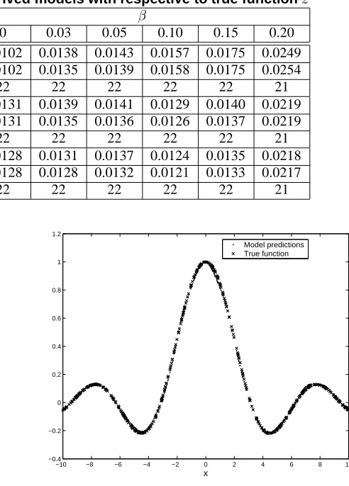
Figure 2. The Bisquare M-estimator model predictions with <; 0
and true functions.
1000 training data
)
were generated from
)
-B+
)
, using uniformly distributed random ) (
"
G; #G;, . The additive noise
is a Gaussian mixture that mixes two types of noises, a larger portion of normal noise with smaller variance and a smaller portion of noise with higher vari-ance. i.e.
%>; ; 0
4
@
"
@%>; ; 0;83
4
, where
;
1 1 ; 0
as a small number to denote the contamina-tion ratio, such that
has the probability @
"
of being drawn from%>; ; 0;83
4
( as “normal ”), and a probability of%>; ; 0
4
(as “outliers ”).
For various levels of contamination ratio , 1000 noisy observations were generated and divided into a training data set of 500 data points and a test data set of 500 data points. The 500 training data points is shown in Fig.1 for different . For each case, the proposed algorithm is applied based on the RBF network. All the training data points are used as the candidate centre set
Y
’s, with
constructed using Gaussian function
)
W
" =
)
= 4 4
[
. The width
is fixed for simplicity. Note that by removing the IRLS inner loop of the algorithm, the procedure simply reduces to OFR with D-optimality algo-rithm [10]. With various values of as different level of bad data conditions, the proposed algorithm is compared with OFR with D-optimality algorithm using only least squares estimates and SVM regression. All of the derived models based on OFR algorithm have the number of centers in the range of0 /
?!
. The root of mean squares (RMS) errors of a range of data conditions are listed in Table 1. It is seen that the proposed algorithm is most robust to out-liers when the data contains approximately G;:
outliers. To achieve better performance for M-estimators, it is useful to slightly adjust tuning constants because these are set for
9
38:
efficiency when data is normal. As data distribution is unknown these values can be adjusted via iterations and cross-validation. For the training data set with ; 0
, the model predicted output by using the proposed algorithm with Turkey bisquare M-estimators is shown in Fig.2.
5
Conclusions
In this paper a new orthogonal forward regression (OFR) model identification algorithm has been introduced. The orthogonal forward regression (OFR), often based on the modified Gram-Schmidt procedure, is an efficient method incorporating structure selection and parameter estima-tion simultaneously. The proposed algorithm includes M-estimator by using an iterative re-weighted least squares (IRLS) algorithm inner loop based on the modified Gram-Schmidt procedure. D-optimality as a model structure ro-bustness criterion is used in model selection. In this manner the proposed approach extends the use of the OFR algo-rithm for parsimonious model structure determination even in bad data conditions via the derivation of parameter M-estimators with inherent robustness to outliers.
Acknowledgement The authors gratefully acknowledge that part of this work was supported by EPSRC in the UK.
References
[1] M. Brown and C. J. Harris. Neurofuzzy Adaptive Modelling
and Control. Prentice Hall, Hemel Hempstead, 1994.
[2] J. H. Chen, C. S. Chen, and Y. S. Chen. Fast algorithm for robust template matching with m-estimators. IEEE Trans.
on Signal Processing, 51(1):230–243, 2003.
[3] S. Chen, S. A. Billings, and W. Luo. Orthogonal least
squares methods and their applications to non-linear system identification. International Journal of Control, 50:1873– 1896, 1989.
[4] S. Chen, X. Hong, and C. J. Harris. Sparse kernel regression modelling using combined locally regularised orthogonal least squares and d-optimality experimental design. IEEE
Trans. on Automatic Control, 48(6):1029–1036, 2003.
[5] S. Chen, Y. Wu, and B. L. Luk. Combined genetic algo-rithm optimization and regularized orthogonal least squares learning for radial basis function networks. IEEE Trans. on
Neural Networks, 10:1239–1243, 1999.
[6] J. T. Connor and R. D.Martin. Recurrent neural networks and robust time series prediction. IEEE Transactions of
Neu-ral Networks, 5(2):240–253, 1994.
[7] A. B. Hamza, H. Krim, and G. B. Unal. Unifying proba-bilistic and variational estimation. IEEE Signal Processing
Magazine, 19(September):37–47, 2002.
[8] C. J. Harris, X. Hong, and Q. Gan. Adaptive Modelling,
Estimation and Fusion from Data: A Neurofuzzy Approach.
Springer-Verlag, 2002.
[9] X. Hong, M. Brown, S. Chen, and C. J. Harris. Sparse model identification using orthogonal forward regression with ba-sis pursuit and [d]-optimality. Submitted to IEE Proc. -
Con-trol Theory and Applications, 2003.
[10] X. Hong and C. J. Harris. Nonlinear model structure de-sign and construction using orthogonal least squares and d-optimality design. IEEE Transactions on Neural Networks, 13(5):1245–1250, 2001.
[11] X. Hong, C. J. Harris, S. Chen, and P. M. Sharkey. Robust nonlinear model identification methods using forward regre-sion. IEEE Transactions on Systems, Man, and Cybernetics,
Part A, 33(4):514–523, 2003.