R. G. Ingalls, M. D. Rossetti, J. S. Smith, and B. A. Peters, eds.
EFFICIENT PRICING OF BARRIER OPTIONS WITH THE VARIANCE-GAMMA MODEL
Athanassios N. Avramidis
Département d’Informatique et de Recherche Opérationnelle Université de Montréal, C.P. 6128, Succ. Centre-Ville
Montréal, H3C 3J7, CANADA
ABSTRACT
We develop an efficient Monte Carlo algorithm for pricing barrier options with the variance gamma model (Madan, Carr, and Chang 1998). After gener-alizing the double-gamma bridge sampling algorithm of Avramidis, L’Ecuyer, and Tremblay (2003), we develop conditional bounds on the process paths and exploit these bounds to price barrier options. The algorithm’s efficiency stems from sampling the process paths up to a random res-olution that is usually much coarser than the original path resolution. We obtain unbiased estimators, including the case of continuous-time monitoring of the barrier crossing. Our numerical examples show large efficiency gain relative to full-dimensional path sampling.
1 INTRODUCTION
Madan and Seneta (1990), Madan and Milne (1991) and Madan, Carr, and Chang (1998) developed the variance gamma (VG) model with application to modeling asset returns and option pricing. The variance gamma process is a Brownian motion with random time change, where the random time change is a gamma process, i.e., a continuous-time process with stationary, independent gamma increments. It was argued that the variance gamma model permits more flexibility in modeling skewness and kurtosis relative to Brownian motion. Closed-form solutions for European option were developed and empirical evidence was provided that the VG option pricing model gives a better fit to market option prices than the classical Black-Scholes model. Except for European options, pricing with variance gamma generally requires numerical techniques; such techniques were developed in Hirsa and Madan (2004) for American options and Ribeiro and Webber (2004), Avramidis, L’Ecuyer, and Tremblay (2003) for path-dependent options.
Bridge samplingof the variance gamma process was in-dependently proposed by Ribeiro and Webber (2004) and Avramidis, L’Ecuyer, and Tremblay (2003) and combined
with stratification and Quasi-Monte Carlo, respectively, for pricing path-dependent options efficiently. Large ef-ficiency gains were demonstrated for Asian and look-back options. For barrier options, the results reported in Ribeiro and Webber (2004) do not give a complete picture, but imply the efficiency gain essentially disappears as the barrier approaches the initial asset price.
When the option contract specifies continuous monitor-ing of the barrier crossmonitor-ing, Monte Carlo-based estimators are generally biased due to the simulation’s discrete-time monitoring. For option-pricing models driven by more gen-eral Lévy processes, Ribeiro and Webber (2003) develop a correction method for the simulation bias. While empiri-cally found effective, their approach is heuristic and does not yield error bounds, so there is a risk of increasing the error relative to the uncorrected procedure.
Our method is based on double-gamma bridge sampling (DGBS) of a variance gamma process (Avramidis, L’Ecuyer, and Tremblay 2003). With DBGS, conditional on sampled values of two gamma processes at any finite set of times containing 0 andT, we can compute bounds on the VG path everywhere on (0, T]. For many payoff functions arising in applications, these process-path bounds translate into lower and upper bounds on the con-ditional payoff; in this paper, we focus on barrier options to convey the main ideas. The algorithm samples a path of the VG process until the gap between the bounding es-timators is closed; this ensures unbiasedness, including the case of continuous monitoring of the barrier crossing. In numerical examples, we show that the algorithm’s expected work is considerably reduced relative to full-dimensional path sampling.
Section 3.3 analyzes the particular case of barrier options. In Section 4 we demonstrate the efficiency gain with two numerical examples.
2 OPTION PRICING WITH VARIANCE GAMMA
Under the variance gamma model, the asset log-return dy-namics are characterized by a continuous-time stochas-tic process obtained as a subordinate to Brownian mo-tion, where the random time change (called operational time in Feller (1966)) obeys a gamma process. Let B = {B(t;θ, σ ) : t ≥ 0} be a Brownian motion with drift parameter θ and variance parameter σ. Let G = {G(t;µ, ν) : t ≥ 0}denote a gamma process with mean rate µand variance rateν; this is a process with indepen-dent gamma increments with G(t+h;µ, ν)−G(t;µ, ν) having mean µh and variance νh. The variance gamma (VG) process X(t;θ, σ, ν)is defined as
X(t;θ, σ, ν):=B(G(t;1, ν), θ, σ ).
whereG(t;1, ν)is a unit-mean gamma process independent of B.
Option prices under the VG model are expectations of functionals of paths of the asset price process, where expec-tations are taken with respect to the risk-neutral measure. Under the risk-neutral dynamics, the asset-price processS has paths
S(t )=S(0)exp{(ω+r−q)t+X(t )},
whereXis a VG process,ris the continuously-compounded, risk-free interest rate, q is the asset’s continuously-compounded dividend yield, andω=log(1−θ ν−σ2ν/2)/ν ensuresthatE[S(t)]=S(0) exp[(r−q)t].Inpractice,parameter values θ,σ and ν are estimated by calibrating the model against observed option prices. For a more detailed review, see Madan, Carr, and Chang (1998).
3 ALGORITHM AND PROPERTIES
3.1 Generalized Double Gamma Bridge Sampling
The VG process paths have a representation as the difference between two independent gamma processes (Madan, Carr, and Chang 1998):
X(t;θ, σ, ν)=+(t;µp;νp)−−(t;µn;νn), (1)
where+ and−are independent gamma processes with
µp = (1/2)
θ2+2σ2/ν+θ/2 µn = (1/2)
θ2+2σ2/ν−θ/2
νp =
(1/2)
θ2+2σ2/ν+θ/2 2
ν
νn =
(1/2)
θ2+2σ2/ν−θ/2 2
ν.
The two gamma processes have common shape parameter per unit-time increment,µ2p/νp=µ2n/νn=1/ν.
Based on the above representation, Avramidis, L’Ecuyer, and Tremblay (2003) developed double-gamma bridge sampling (DGBS) of a VG process. Their algorithm was stated for dyadic partitions of the target time horizon; we make a direct generalization for sampling an arbitrary time partition. We consider a finite time interval[0, T]and in infinite sequence of distinct real numbers yo =0, y1 =T, and y2, y3,..., dense in(0, T ). This is the sequence of time points at which the two gamma processes are sampled (generated), in order: first at y1; then aty2, conditional on their values aty1; then aty3, conditional on their values aty1andy2; and so on. For each positive integer m, let 0=tm,0< tm,1 < . . . < tm,m =T denote the valuesyo,y1,. . .,ymsorted by increasing order, and let ι(m)be the index i such thattm,i =ym. That is, tm,ι(m) is the new observation time added at stepm.
We call this more general sampling method the general-ized DGBSalgorithm. Figure 1 outlines the algorithm with an infinite loop. In an actual implementation, the algorithm can be stopped after any number of steps.
3.2 Bounds on the Asset-Price Process
Define
ζ = ω+r−q ζ+ = max(ζ,0) ζ− = max(−ζ,0)
and recall the asset-price processS has representation
S(t ) = S(0)exp[ζ t+X(t )]
= S(0)exp[ζ t++(t )−−(t )], t ≥0,(2)
where+and−are the gamma processes in (1). Define
t1,0←0; t1,1←T; +(0)←0; −(0)←0 Generate+(T )∼Gamma(T /ν, νp/µp) Generate−(T )∼Gamma(T /ν, νn/µn) Form=2 to ∞{
i←ι(m) tm,i ←ym
tm,i−1←tm−1,i−1; tm,i+1←tm−1,i
α1←(ym−tm,i−1)/ν; α2←(tm,i+1−ym)/ν GenerateY+∼Beta(α1, α2)
+(ym)←+(tm,i−1) ++(tm,i+1)−+(tm,i−1)
Y+
GenerateY−∼Beta(α1, α2) −(ym)←−(tm,i−1)
+−(tm,i+1)−−(tm,i−1)
Y−
[image:3.612.39.275.62.314.2]X(ym)←+(ym)−−(ym) }
Figure 1: Generalized Double Gamma Bridge Sampling of a VG ProcessX with Parameters(1, ν, θ, σ )at an Infinite Sequence of Timesyo=0,y1=T, andy2,y3,... in(0, T]
and
Lm,i = S(tm,i−1)exp[−ζ−(tm,i−tm,i−1)−m,i− ], Um,i = S(tm,i−1)exp[ζ+(tm,i−tm,i−1)+m,i+ ], Lm(t ) = Lm,i,
Um(t ) = Um,i,
for tm,i−1< t < tm,i, and Lm(tm,i)=Um(tm,i)=S(tm,i), for i=1, . . . , m.
The following proposition states that the processS is contained between the piecewise constant processes Lm and Um and that these pathwise bounds are narrowing monotonically withm.
Proposition 1 For every sample path of S, any integerm≥1, and allt ∈ [0, T], we have
Lm(t )≤Lm+1(t )≤S(t )≤Um+1(t )≤Um(t ). Proposition 1 is a consequence of (2) and the fact that the gamma increments are nonnegative. Avramidis and L’Ecuyer (2004) state bounding processes that are tighter bounds thanLmandUm. The current result is obtained as their Corollary 1.
3.3 Barrier Options
We start with a basic description of the different types of barrier options. Aknock-inoption comes into existence only if the underlying asset price crosses a given barrier. A knock-out option ceases to exist whenever the underlying asset price crosses a barrier. Further, we distinguish them asupor down, depending on the direction of asset-price movement that triggers the barrier crossing. They are further classified as call orput. For further information, see Hull (2000).
As a prototypical barrier option, we consider the up-and-in callwith continuous monitoring of the barrier crossing; the payoff, discounted to time zero, is
CB(∞)=e−rT (S(T )−K)+I
sup 0≤t≤T
S(t ) > b
, (3)
where b > S(0) is thebarrier,K is the strike price, and I denotes the indicator function. The related option with discrete monitoring has discounted payoff
CB(d)=e−rT (S(T )−K)+I
max
1≤i≤dS(ti) > b (4)
for given ti ∈(0, T],i=1, . . . , d. Define the sequence of estimators
CL,m=e−rT (S(T )−K)+I
max
1≤i≤mS(tm,i) > b
and
CU,m=e−rT(S(T )−K)+I
max
1≤i≤mUm,i> b ,
for m = 1,2, . . .. An interesting feature of this pair of estimators is that the gap between them vanishes ifS(T )≤K or if the indicator function takes the same value in both cases, i.e., whenever
max
1≤i≤mS(tm,i) > b or 1max≤i≤mUm,i ≤b. (5) Thus, to estimate the continuous-time price, it appears sen-sible to continue sampling until this gap is closed. LetM denote the random variable defined as the smallest m for which (5) holds. To allow additional deterministic truncation of sampling after ksteps, define
M(k)=min(M, k). (6)
1. Let
Fm=(+(tm,1), −(tm,1), . . . , +(tm,m), −(tm,m)).
Proposition 2 (a) For any fixed m≥1, con-ditional onFm,
CL,m≤CB(∞)≤CU,m. Moreover,
CL,m≤CB(d)≤CU,m whenever
{tm,1, . . . , tm,m} ⊆ {t1, . . . , td}. (7)
The bounding estimators are narrowing monoton-ically inm.
(b) The estimatorCL,M(∞)=CU,M(∞)is unbiased for the continuous-time price E[CB(∞)]. Moreover, CL,M(d) =CU,M(d) is unbiased for the discrete-time priceE[CB(d)]whenever (7) holds.
Part (b) states an attractive property of unbiased-ness for the case of continuous-time monitoring; this was precisely the goal of the correction procedure of Ribeiro and Webber (2003), which, however, doesnot guar-antee unbiasedness. On the other hand, an unresolved issue in our procedure is whether M(∞) has finite mean. For the case of discrete-time monitoring with finite but larged, our unbiased estimator is likely to require considerably less computation compared to the unbiased estimator that sam-ples full-dimensional paths; empirical evidence supporting this assertion is offered in Section 4. Moreover, part (a) shows a pair of estimators whose expectations bracket the option price; this permits constructing confidence intervals that may be useful in time-critical applications where some pricing accuracy is exchanged for speed of computation.
The above approach and results analogous to Proposition 2 apply with very straightforward modifications to the other types of barrier options. For example, for adown-and-in call option, we haveb < S(0), we replace “sup0≤t≤T S(t ) > b” in the indicator function in (3) by “inf0≤t≤TS(t ) < b”, and make corresponding replacements in the low and high estimators. The additional variationsup-and-out call, down-and-out call, and theputversions can be handled similarly.
4 NUMERICAL RESULTS
We examine the efficiency of the estimator in Proposi-tion 2(b) for two examples of barrier opProposi-tions with discrete
monitoring. We consider the up-and-in call (4) and the down-and-out call with discounted payoff
e−rT (S(T )−K)+I
min
1≤i≤dS(ti) > b .
Both options have discrete monitoring at ti =T i/d, i = 1, . . . , d. Option parameters are: S(0)=100 andK=100.
We take VG model parameters from
Hirsa and Madan (2004): T = 0.46575, σ = 0.19071, ν =0.49083, θ= −0.28113,r =0.0549, andq =0.011; these were calibrated against options on the S&P 500 index using data for June 30, 1999 and correspond to intermediate-maturity options.
Given the estimator’s unbiasedness, the efficiency gain factor compared to full-dimensional (non-truncated) sam-pling is the ratio of expected work between the two es-timators. Tables 1 and 2 show results for the up-and-in call and the down-and-out call, respectively; we give 95% confidence intervals on the expected work E[M(d)] and the estimated option prices, varying the barrier b and the problem dimensiond. The ratiod/E[M(d)]may be viewed as a simple, albeit rough, measure of the efficiency gain. In all cases, we see that expected work grows very slowly with the dimensiond; equivalently, efficiency increases rapidly.
Table 1: Estimated Expected Work E[M(d)] and Price (Standard Error in Parentheses) for Up-and-in Call Option, for Selected Barrier Levels b and Dimensiond.
b d 95% C.I. on E[M(d)] Price
105 4 ( 2.20, 2.20) 7.3329 ( 0.008)
16 ( 3.64, 3.65) 7.3739 ( 0.008)
64 ( 5.10, 5.13) 7.3843 ( 0.008)
256 ( 6.54, 6.61) 7.3874 ( 0.008)
110 4 ( 2.25, 2.26) 6.3883 ( 0.008)
16 ( 3.55, 3.56) 6.5260 ( 0.008)
64 ( 4.83, 4.86) 6.5716 ( 0.008)
256 ( 6.09, 6.15) 6.5833 ( 0.008)
120 4 ( 2.11, 2.11) 2.0406 ( 0.006)
16 ( 2.41, 2.42) 2.1238 ( 0.007)
64 ( 2.71, 2.73) 2.1557 ( 0.007)
256 ( 3.01, 3.04) 2.1654 ( 0.007)
[image:4.612.311.529.413.573.2]Table 2: Estimated Expected Work E[M(d)] and Price (Standard Error in Parentheses) for Down-and-out Call Option, for Selected Barrier Levels b and Dimensiond.
b d 95% C.I. on E[M(d)] Price
80 4 ( 2.16, 2.16) 7.5018 ( 0.008)
16 ( 2.45, 2.46) 7.5011 ( 0.008)
64 ( 2.74, 2.76) 7.5008 ( 0.008)
256 ( 3.03, 3.06) 7.5007 ( 0.008)
95 4 ( 2.49, 2.49) 7.3199 ( 0.008)
16 ( 3.45, 3.47) 7.1832 ( 0.008)
64 ( 4.42, 4.44) 7.1368 ( 0.008)
256 ( 5.36, 5.41) 7.1241 ( 0.008)
99 4 ( 2.77, 2.77) 6.8283 ( 0.007)
16 ( 4.47, 4.49) 6.3299 ( 0.007)
64 ( 6.20, 6.24) 6.1528 ( 0.007)
256 ( 7.93, 8.00) 6.1021 ( 0.007)
In the least-favorable (smallest-distance) case across our experiments, the down-and-out option withb=99, we get E[M(256)] ≈8. This should be contrasted to the negative results of Ribeiro and Webber (2004), who found little or no efficiency gain when distance is small.
REFERENCES
Avramidis, A. N., and P. L’Ecuyer. 2004. Efficient Monte Carlo and Quasi-Monte Carlo option pricing with the variance-gamma model. Working paper, Department of Computer Science and Operations Research, Université de Montréal.
Avramidis, A. N., P. L’Ecuyer, and P.-A. Tremblay. 2003. Efficient simulation of gamma and variance-gamma processes. InProceedings of the 2003 Winter Simulation Conference, ed. S. Chick, P. J. Sanchez, D. Ferrin, and D. J. Morrice, 319–326. Piscataway, New Jersey: IEEE Press.
Feller, W. 1966.An introduction to probability theory and its applications, vol. 2. first ed. New York: Wiley. Hirsa, A., and D. B. Madan. 2004. Pricing American options
under variance gamma.The Journal of Computational Finance 7 (2):63–80.
Hull, J. 2000. Options, futures, and other derivative secu-rities. fourth ed. Englewood-Cliff, N.J.: Prentice-Hall. Madan, D. B., P. P. Carr, and E. C. Chang. 1998. The variance gamma process and option pricing.European Finance Review 2:79–105.
Madan, D. B., and F. Milne. 1991. Option pricing with V.G. martingale components. Mathematical Finance 1:39– 55.
Madan, D. B., and E. Seneta. 1990. The variance gamma (V.G.) model for share market returns.Journal of Busi-ness63:511–524.
Ribeiro, C., and N. Webber. 2003. Correcting for simulation bias in Monte Carlo methods to value exotic options in models driven by Lévy processes. Working Paper, Cass Business School, London, UK.
Ribeiro, C., and N. Webber. 2004. Valuing path-dependent options in the variance-gamma model by Monte Carlo with a gamma bridge. The Journal of Computational Finance 7 (2):81–100.
AUTHOR BIOGRAPHY
[image:5.612.48.260.115.274.2]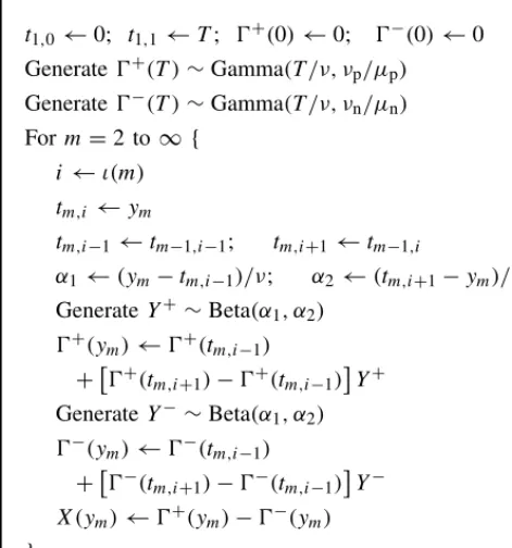
![Table 1:Estimated Expected Work E[M(d)] andPrice (Standard Error in Parentheses) for Up-and-in Call Option, for Selected Barrier Levels b andDimension d.](https://thumb-us.123doks.com/thumbv2/123dok_us/8515510.351465/4.612.311.529.413.573/estimated-expected-andprice-standard-parentheses-selected-barrier-anddimension.webp)
![Table 2:Estimated Expected Work E[M(d)] andPrice (Standard Error in Parentheses) for Down-and-out Call Option, for Selected Barrier Levels b andDimension d.](https://thumb-us.123doks.com/thumbv2/123dok_us/8515510.351465/5.612.48.260.115.274/estimated-expected-andprice-standard-parentheses-selected-barrier-anddimension.webp)
