Nonlinear Output Feedback Control for Robust Stability

Nonlinear Output Feedback Control for Robust Stability

Chengkang Xie and Mark French

Abstract— In the presence of input and measurement distur-bances, an observer and a controller are designed to achieve robust stability for the nominal plant in normal form. By framework of nonlinear gap metric, a robust margin of plant perturbations is obtained, and the controller is shown to be robust to plant perturbations if the gap metric is less than the robust margin.

I. INTRODUCTION

In general, to control a physical plant, a mathematical model ( called the nominal plant ) for the plant is neces-sary. But, in practice, the nominal plant cannot completely describe the physical plant, there always exists a plant perturbation. In operation of control, sensors and actuators are setup to measure and input signals, and the sensors and actuators result in measurement errors and input errors, namely, measurement disturbances and input disturbances. A closed-loop could become unstable if a controller cannot tolerate these kinds of uncertainties. EI-Sakkary [1] gave an example that a small uncertainty changed the stability of the closed-loop. So, for control purposes, a basic requirement is that a controller designed for the nominal plant tolerates plant perturbations, measurement disturbances and input dis-turbances, that is the controller is robust to these kinds of uncertainties.

Although the study of robustness for control designs is as old as feedback control, even for linear systems effective systematic tools for robust control have only been devel-oped since 1980’s. An appropriate topological structure for studying the robustness of linear systems is the gap metric ( graph topology ) introduced by Zames and EI-Sakkary [8], [1]. In contrast, other frameworks for studying robustness have restrictions; e.g., the order of parametric uncertainty cannot be changed, a small time delay is not an allowable uncertainty, Un-modeled dynamics or plant perturbations are not allowed, etc.. For nonlinear control, it is difficult to cope with the complexity of nonlinear phenomena even in the absence of disturbances and other uncertainties, the robustness study of nonlinear systems is far less developed than for linear systems. In 1997, Georgiou and Smith [4] established a theory of gap metric for nonlinear case. It provides a powerful tool to study robustness of nonlinear

C. Xie is with Institute of Mathematics, Southwest University, Beibei, Chongqing, 400715, P.R. China;[email protected]. The author was supported by the Natural Science Foundation of Chongqing under Grants CSTC 2005EB2048.

M. French is with School of Electronics and Computer Sci-ence, University of Southampton, Southampton, SO17 1BJ, UK;

[email protected]

control. Via the framework of nonlinear gap metric, Xie and French [7] successfully designed a robust backstepping controller for state feedback in 2003. Any restrictions on disturbances and plant perturbations have been removed, and the disturbances and perturbations can be un-modeled dynamics. So, it presents that the framework of nonlinear gap metric is a appropriate topological structure for nonlinear feedback control.

In the past two decades, many of control techniques have been developed for nonlinear systems using feedback control. Most of the results, however, assume full state feedback. Efforts to extend some of these results to output feedback have naturally included the idea of designing an observer to estimate the state of a system from its output, see, e.g., [5], [2], [6], [3]. It is a meaningful work to utilize the framework of nonlinear gap metric for the study of output feedback control.

In this paper, we consider a nominal plant in normal form and design an observer and a controller to achieve robust stability of the closed-loop system in the presence of input and measurement disturbances. Then we utilize the results in [4] to obtain the robustness of the closed-loop to plant perturbations which are small in the sense of the gap metric. That is, we show that the controller stabilizes the closed-loop for any perturbed plant in the presence of input and measurement disturbances if the gap metric distance between the nominal and perturbed plant is less than a computable constant. Any restrictions on input and measurement disturbances, and plant perturbations have been removed, and the disturbances and perturbations can be un-modeled dynamics.

II. BACKGROUND ANDPROBLEMFORMULATION

In this section we first simply state the background for gap metric robustness. The material here comes from the fundamental paper [4].

A. Background for Gap Metric Robustness

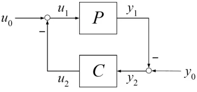
Let U and Y be normed signal spaces, and consider a causal nominal plant

P : U → Y: u₁→y₁ and a causal controller

C: Y → U : y₂→u₂

In a control system, there exist measurement disturbance y₀∈ Y and input disturbance u₀∈ U, which are uncertain-ties. The standard feedback configuration is shown in Fig. 1,

Proceedings of the

44th IEEE Conference on Decision and Control, and the European Control Conference 2005

Seville, Spain, December 12-15, 2005

Fig. 1. Standard Feedback Configuration

and the signals have relations:

y₁=Pu₁, u₂=Cy₂ y₀=y₁+y₂, u₀=u₁+u₂

LetW denoteU × Y, and write

w₀=

u₀ y₀

, w₁=

u₁ y₁

, w₂=

u₂ y₂

Thus the closed-loop operator is defined by

H_P,C : W → W × W: w₀→(w₁, w₂)

The graph of the plantP is defined as

GP =

u

Pu

: u∈ U

⊂ W

and the graph of the control operatorC is defined as

GC=

Cy

y

: y∈ Y

⊂ W

For simplicity of notation, normally, we writeG_P asM, and

GC asN respectively.

To define robust stability of the closed-loop to distur-bances, let Πi be the natural projection of W × W onto theith component ( i= 1,2 ), another tow operators

ΠM//N = Π1HP,C , ΠN//M= Π2HP,C

are introduced, that is

ΠM//N : W → W: w0→w1 ΠN//M: W → W: w0→w2

Definition 1: The closed-loop[P,C]is said to be stable if the operatorΠ_M//N has a finite induced norm, i.e.

ΠM//N= sup w0=0

ΠM//Nw0

w₀ = sup_w0=0

w₁

w₀ <∞ The notion of stability for nonlinear control is a strong requirement. It can be relaxed to gain-function stability as follows.

Definition 2: The gain-function of the operatorΠ_M//N is defined as

g[Π_M//N](α) = sup

w0≤α

ΠM//Nw0, α≥0

The closed-loop [P,C] is said to be gain-function ( gf- ) stable ifg[Π_M//N](α)remains finite for allα≥0.

It can be seen that if there exists a positive constantΓsuch that

w₁ ≤Γw₀, w₁, w₀∈ W (1)

then[P,C]is stable; if there exists a continuous function γ(·)>0 such that

w₁ ≤γ(w₀), w₁, w₀∈ W (2)

then[P,C]is gf-stable.

Finally, we define the gap metric between the nominal plantP and any perturbed plantP1 as follows.

Definition 3: For plant P and plant P₁, the directed gap metric between the two plants is defined as

δ(P,P₁) =

infΦ∈O(Φ−I)|M, if O =∅

∞, if O=∅

and the gap metric is defined as

δ(P,P₁) = max{δ(P,P₁), δ(P₁,P)}

where

O={Φ :M → M1|Φis causal, bijective andΦ(0) = 0}

andM₁ is the graph of P₁, namelyG_P1.

The significance of the introduction of gap metric lies in the following theorem.

Theorem 1: For the feedback system in Fig. 1, let the closed-loop[P,C]be stable. If a plantP₁ is such that

δ(P,P1)< 1

ΠM//N

then the closed-loop[P₁,C]is also stable, and

ΠM1//N ≤ ΠM//N

1 +δ(P,P1) 1− ΠM//Nδ(P,P1)

The proof of this theorem can be found in paper [4]. Definition 1, 2, and Theorem 1 provide a complete frame-work to design a robust controller in the presence of input, measurement disturbances, and plant perturbations. First, for the nominal plant P design a controller C such that the closed-loop operator H_P,C is stable, namely, the operator ΠM1//N has a finite induce norm, or the signals satisfy

(1). Second, by Theorem 1, we get a plant robust margin

ΠM1//N−1, the controllerCthus can stabilize any

B. Problem Formulation

Consider following nominal plant in normal form

P(x0₁) : ˙x₁₁=x₁₂ .. . ˙

x_1(n−1)=x_1n (3)

˙

x_1n=ϕ(x₁₁,· · ·, x_1n) +u₁ y₁=x₁₁

where

x0₁= (x0₁₁,· · ·, x0_1n)T

is the initial condition. Well-posedness of the differential equations grantees that of the feedback configuration, hence, for the well-posedness of the differential equations, we assume that ϕ(0) = 0, and ϕ is Lipschitz continuous, that is, there exist a constantLsuch that for anyω₁, ω₂∈Rn, it hold

|ϕ(ω1)−ϕ(ω2)| ≤Lω₁−ω₂

where we utilize · to denote the Euclid norm. We introduce following notations

x₁=

⎛ ⎜ ⎜ ⎜ ⎝

x₁₁ x₁₂ .. . x1n

⎞ ⎟ ⎟ ⎟ ⎠, A=

⎛ ⎜ ⎜ ⎜ ⎜ ⎝

0 1 0 · · · 0 0 0 0 1 · · · 0 0 . . . . 0 0 0 · · · 0 1 0 0 0 · · · 0 0

⎞ ⎟ ⎟ ⎟ ⎟ ⎠, B=

⎛ ⎜ ⎜ ⎜ ⎝

0 .. . 0 1

⎞ ⎟ ⎟ ⎟ ⎠

C= (1,0,· · ·,0)

then the plant can be rewrite as

P(x0

1) : ˙x1=Ax1+B(ϕ(x1) +u1), x1(0) =x01 (4a)

y₁=Cx₁ (4b)

Take signal spaces

U =L∞(R), Y =L∞(R)

then

P(x0

1) : L∞(R)→L∞(R) : u1→y1

The norm for the spaceL∞(R)is defined as the normal norm

· ∞.

The problem is to design a controller such that the closed-loop system is stable or gf-stable. Alternatively, such that there exist a constantΓand a gain functionγ(·)which satisfy (1) and (2).

III. DESIGN OFCONTROLLER

Firstly, we chose a vector

K= (k₁,· · ·, k_n)

such that A₀ = A+BK is Hurwitz. Secondly, we chose positive constantsα_i, i= 1,· · ·, nsuch that the roots of the equation

sn+α₁sn−1+· · ·+α_n−1s+α_n= 0

are in the left-half plane, and let

D= (α₁, α₂,· · ·, α_n)T

Then we design an observer as ˙ˆ

x₂=Aˆx₂−D(y₂−yˆ₂) +BKxˆ₂, xˆ₂(0) = ˆx0₂ (5a) ˆ

y₂=Cˆx₂ (5b)

Lastly, we define a controller as

C(ˆx0₂) :

u₂=ϕ(−y₂) +Kxˆ₂ (6a)

˙ˆ

x2=Aˆx2+D(y2−yˆ2) +BKxˆ2, xˆ2(0) = ˆx0₂ (6b) ˆ

y₂=Cˆx₂ (6c)

IV. ROBUSTNESSANALYSIS

First we prove a lemma about the estimate of the observer error.

Lemma 1: Letx₁ be the state of the plant in (4), andxˆ₂ be observer state in (5), and let

˜

x=x₁+ ˆx₂

be the perturbed observer error. Then there exist positive constantsb andβ such that

x˜_∞≤bx˜0+β(u₀, y₀)T_∞ (7) where

˜

x0=x0₁+ ˆx0₂

Proof: Note that

u₁=u₀−u₂, y₂=y₀−y₁

then the closed-loop[P(x0₁),C(ˆx0₂)]can be written as

˙

x₁=Ax₁+Bϕ(y₁)−ϕ(−y₂)−Kˆx₂+u₀, x₁(0) =x0₁ ˙ˆ

x2=Aˆx2+Dy0−C(x1+ ˆx2)+BKxˆ2, xˆ2(0) = ˆx0₂

From above two equations, we obtain ˙˜

x=A₁x˜+Dy₀+B(ϕ(y₁)−ϕ(−y₂)+u₀), x(0) = ˜˜ x0 (8)

where

A₁=A−DC

Solving (8), we obtain

˜

x=eA1t_x˜0+ _t

0 e

A1(t−τ)×

Dy0(τ) +B

ϕy1(τ)−ϕ−y2(τ)+u0(τ)

dτ (9)

SinceA₁ is Hurwitz, all the real parts of the eigenvalues of A₁ are negative. We take a positive constantµ such that

−µis greater than all the real parts of the eigenvalues ofA₁, then there exists a positive constantbsuch that

eA1t ≤_be−µt

On the other hand, by Lipschitz condition, it holds that

|ϕ(y1)−ϕ(−y2)| ≤L|y₁+y₂|=L|y₀|

Therefore, from (9), we obtain

x(t)˜

≤x˜0 · eA1t+ _t

0 dτe

A1(t−τ)×

Dy0(τ)+ϕ(y1(τ))−ϕ(−y2(τ))+u0(τ)

≤x˜0be−µt

+

_t

0 be

−µ(t−τ)_(D+L)y

0∞+u0∞dτ

≤bx˜0+ b µ

(D+L)y_0∞+u_0∞

≤bx˜0+β(u₀, y₀)T_∞

Write

β=b

√

2

µ max{D+L,1}

then we obtain (7), and complete the proof. Now we state and prove the main result.

Theorem 2: Let the plant P(x0₁) and controller C(ˆx0₂) be defined by (3) and (6). Then

1) There exists a continuous functionγ:R3₊→[0,+∞) such that for all (u0, y0)T∈L∞(R+)×L∞(R+), it holds

_{(u1, y1)}T

∞≤γ(u0, y0)T∞,x˜0,x01∞

(10) that is, the closed-loop[P(x0₁),C(ˆx0₂)]is gf-stable. 2) If x0₁ is zero, by setting xˆ0₂ to be zero, there

exists a positive constant Γ such that for all (u₀, y0)T∈L∞(R+)×L∞(R+), it holds

_{(u1, y1)}T

∞≤Γ(u0, y0)T∞ (11)

that is, the closed-loop[P(0),C(0)] is stable.

Proof: Let Qbe the solution of the equation

(A+BK)T_{Q+Q(A+BK) =−2I}

and consider the Lyapunov function

V(t) =V(x1)(t) =xT₁Qx₁ (12)

then along the trajectories of the closed-loop, we have ˙

V = ˙xT₁Qx₁+xT₁Qx˙₁

=Ax₁+B(ϕ(y1) +u1)TQx₁ +xT₁QAx₁+B(ϕ(y1) +u1) =Ax₁+Bϕ(y₁) +u₀−u₂TQx₁

+xT₁Q

Ax₁+Bϕ(y1) +u₀−u₂

=Ax₁+Bϕ(y₁) +u₀−ϕ(−y₂)−Kxˆ₂TQx₁

+xT₁Q

Ax₁+Bϕ(y1) +u₀−ϕ(−y2)−Kxˆ₂

=xT₁(A+BK)TQ+Q(A+BK)x₁ + 2BTQx₁ϕ(y1)−ϕ(−y2)−Kx˜+u₀

=−2xT₁x₁+ 2BTQx₁ϕ(y1)−ϕ(−y2)−K˜x+u₀ =−2x₁2+ 2BTQx₁ϕ(y1)−ϕ(−y2)−Kx˜+u₀

Let

Q={q_ij}_n×n

and

q₁= max 1≤j≤n{|q1j|}

then

BTQx₁≤q₁x₁

On the other hand, from the Lipschitz condition and Lemma 1, we obtain

ϕ(y1)−ϕ(−y2)−Kx˜+u₀

≤Ly_0∞+Kx˜_∞+u_0∞

≤l√2(u₀, y₀)T_∞+Kbx˜0+β(u₀, y₀)T_∞

≤b∗x˜0+β∗(u₀, y₀)T_∞

where

l= max{L,1}

b∗=Kb

β∗ =l√2 +Kβ

Hence

2BTQx₁ϕ(y1)−ϕ(−y2)−Kx˜+u₀

≤2q1b∗x˜0+β∗(u0, y0)T∞x1

Therefore ˙

V =−2x₁2+ 2BTQx₁ϕ(y1)−ϕ(−y2)−kx˜+u₀

≤ − x₁2− x₁2

By Young’s Inequality, we obtain that ˙

V ≤ −x₁2+q₁2b∗x˜0+β∗(u₀, y0)T_∞2

thenV decreases monotonically outside the compact set

R=x₁∈Rn x₁ ≤q₁b∗x˜0+β∗(u₀, y0)T_∞

So, if

x0₁≤b∗x˜0+β∗(u₀, y0)T_∞

thenV(t)remains inR; if

x0₁> b∗x˜0+β∗(u₀, y₀)T_∞

then V(t) monotonically decreases from t = 0 until x₁ reachesR. Therefore

V(t)≤maxV(x0₁), V

where

V = sup

V(x1)x₁ ≤q₁b∗x˜0+β∗(u₀, y0)T_∞

Note that

λ(Q)x₁2≤V(x1)≤λ¯(Q)x₁2

whereλ(Q), λ(Q)¯ are the maximum and minim eigenvalues of matrixQrespectively, then

supV(x1)x₁ ≤q₁b∗x˜0+β∗(u₀, y0)T_∞ = sup ×

¯

λ(Q)x₁2x₁ ≤q₁b∗x˜0+β∗(u₀, y0)T_∞

=¯λ(Q)b∗x˜0+β∗(u₀, y₀)T_∞2 therefore

x₁ ≤

V

λ(Q) ≤max

⎧ ⎨ ⎩

¯ λ(Q)

λ(Q)x01, X

⎫ ⎬ ⎭

where

X=q₁

¯

λ(Q)b∗x˜0+β∗(u₀, y0)T_∞

Write

g(p, q, r) = max

⎧ ⎨ ⎩

¯ λ(Q) λ(Q)r, q1

¯

λ(Q) (b∗_q+β∗_p)

⎫ ⎬ ⎭

then the above inequality can be rewritten as

x₁ ≤g(u₀, y₀)T_∞,˜x0,x0₁ So

x_1∞≤g(u₀, y₀)T_∞,x˜0,x0₁ since the left hand side of the inequality is a constant.

Therefore we obtain our estimate fory_1∞ as follows.

y_1∞=x_11∞≤ x_1∞

≤g(u₀, y0)T_∞,x˜0,x0₁

Next we estimateu_1∞. First

u₁=u₀−u₂

=u₀−ϕ(−y2)−Kxˆ₂

=u₀+ϕ(y₁)−ϕ(−y₂)−K(x₁+ ˆx₂)−ϕ(y₁) +Kx₁ =u₀+ϕ(y₁)−ϕ(−y₂)−Kx˜−ϕ(y₁) +Kx₁

Note thatϕis Lipschitz, andϕ(0)is zero, hence

u_1∞≤u_0∞+ϕ(y₁)−ϕ(−y₂)_∞+Kx˜_∞ +ϕ(y1)_∞+Kx_1∞

≤u_0∞+Ly₁+y_2∞+Kx˜_∞ +Ly_1∞+Kx_1∞

≤u0∞+Ly0∞

+Kbx˜0+β(u₀, y₀)T_∞ +Lg(u₀, y₀)T_∞,x˜0,x0₁ +Kg(u₀, y0)T_∞,x˜0,x0₁

≤l√2(u₀, y0)T_∞

+Kbx˜0+β(u₀, y0)T_∞

+ (L+K)g(u₀, y₀)T_∞,x˜0,x0₁

Write

h(p, q, r) =l√2p+K(bq+βp) + (L+K)g(p, q, r)

then we obtain

u_1∞≤h(u₀, y₀)T_∞,x˜0,x0₁

Therefore, write

γ(p, q, r) =g(p, q, r)2_{+h(p, q, r)}212

then we have built up the following inequality

(u₁, y1)T_∞=u₁2_∞+u₁2_∞12

≤g(u₀, y0)T_∞,x˜0,x0₁2

+h(u0, y0)T∞,x˜0,x01

212

=γ(u₀, y0)T_∞,x˜0,x0₁

that is, the closed-loop is gf-stable.

Ifx0₁= 0andxˆ0₂= 0, thenx˜0= 0. From the definitions of functionsg andh

g(p,0,0) =q₁β∗

¯ λ(Q)p

hence

h(p,0,0) = (l√2 +kβ)p+ (L+k)g(p,0,0) = (l√2 +kβ)p+ (L+k)q₁β∗p

=

l√2 +kβ+ (L+k)q1β∗

¯ λ(Q)

and

γ(p,0,0)

=g(p,0,0)2+h(p,0,0)212

= q₁β∗

¯ λ(Q)p

2

+

l√2 +kβ+ (L+k)q₁β∗

¯ λ(Q)

p

₂!1 2

=(q2₁(β∗)2¯λ(Q)

+

l√2 +kβ+ (L+k)q₁β∗

¯ λ(Q)

₂1 2

p

Let

Γ =(q2

1(β∗)2λ(Q)¯

+

l√2 +kβ+ (L+k)q1β∗

¯ λ(Q)

21 2

then, it follows that (11) holds.

A robustness to plant perturbations can be given as follows.

Theorem 3: Let the plant P(x0₁) and controller C(ˆx0₂) be defined by (3) and (6). Then there existsΓ>0such that if a plantP1 satisfies

δ(P(0),P1)< _Γ1 (13)

then the closed-loop[P1,C(0)]is also stable, and

ΠM1//N ≤Γ

1 +δ(P(0),P1) 1−Γδ(P(0),P1)

(14)

Proof: By Theorem 2, we have shown that there exists Γ>0 such that

ΠM//N ≤Γ

Then, if

δ(P,P₁)< 1 Γ

it holds that

δ(P,P1)< 1

ΠM//N

Hence, by Theorem 1, the closed-loop [P1,C(0)] is stable, and (14) holds, and the proof is completed.

V. CONCLUSIONS ANDCOMMENTS

Within the framework of nonlinear gap metric, an output feedback control design procedure for robust stability has been established in the presence of input, measurement disturbances, and plant perturbations. Any restriction on input and measurement disturbances is not required. Un-modeled plant perturbations such as time delay are allowable uncertainties. So, the work in this paper shows that the frame-work of nonlinear gap metric is an appropriate topological structure for robust output feedback control designs. This paper therefore represents a start to apply the framework of nonlinear gap metric to output feedback control designs for robust stability.

A global Lipschitz condition is imposed on the nonlin-earity of the nominal plant, which is for a global result of input and measurement disturbances; a relaxation of the requirement to local Lipschitz condition leads a semi-global results.

VI. REFERENCES

[1] A. El-Sakkary,The gap metric: Robustness of stabiliza-tion of feedback systems, IEEE Transaction on Automatic Control30 (1985), no. 3, 240–247.

[2] J. Gauthier, H. Hamouri, and I. Kupka, Observer for nonlinear systems, Proceedings of the 30th IEEE Con-ference on Decision and Control (Brighton, England), IEEE, December 1991, pp. 1483–1489.

[3] J. Gauthier and I. Kupka, Observerty and observer for nonlinear systems, SIAM Journal on Control and Optimization 32(1994), no. 4, 975–994.

[4] T. Georgiou and M. Smith,Robustness analysis of non-linear feedback systems: An input-output approach, IEEE Transactions on Automatic Control 42 (1997), no. 9, 1200–1221.

[5] A. Krener and A. Isidori, Linearization by output and non-linear observers, Systems & Control Letters 3

(1983), no. 1, 47–52.

[6] R. Marino and P. Tomei, Global adaptive output-feedback control of nonlinear systems, part 1: Linear pa-rameterization, IEEE Transactions on Automatic Control

38 (1993), 17–32.

[7] C. Xie and M. French, Gap metric robustness of a backstepping control design, Proceedings of the 42nd IEEE Conference on Decision and Control (Hawaii, USA), vol. 5, December 2003, pp. 5180–5184.