Reduced Complexity Single Carrier Maximum Likelihood Detection for Decision Feedback Assisted Space Time Equalization

REDUCED COMPLEXITY SINGLE-CARRIER MAXIMUM-LIKELIHOOD DETECTION FOR DECISION

FEEDBACK ASSISTED SPACE-TIME EQUALIZATION

A. Wolfgang, J. Akhtman, S. Chen, L. Hanzo

School of ECS Univ. of Southampton, SO17 1BJ, UK.

Tel: +44-23-80-593 125, Fax: +44-23-80-594 508

{

aw03r,yja02r,sqc,lh

}

@ecs.soton.ac.uk

http://www-mobile.ecs.soton.ac.uk

ABSTRACT

A novel Decision-Feedback (DF) aided reduced complexity

Maximum Likelihood (ML) Space-Time Equalizer (STE)

de-signed for single-carrier multiple antenna assisted receivers

is introduced. The proposed receiver structure is based on a

recursive tree search, which is capable of achieving ML

per-formance at a moderate computational cost and substantially

outperforms the linear benchmarker based on the Minimum

Mean-Squared Error (MMSE) criterion. Additionally a further

complexity reduction scheme is proposed, which exploits the

specific characteristics of both the wide-band channel and the

proposed DF-STE.

I. INTRODUCTION

In [1] a novel tree search based reduced complexity Maximum

Likelihood (ML) detector designed for Orthogonal Frequency

Divi-sion Multiplexing (OFDM) [2] systems has been introduced, which

is referred to as the Optimized Hierarchical Recursive Search

Algorithm (OHRSA). The OHRSA constitutes an evolution of the

sphere decoder [3], which describes the system’s transfer function

using an upper triangular matrix and then detects the signal on a

dimension by dimension basis. In contrast to conventional sphere

decoding [3], the OHRSA retains its low complexity even in

heavily overloaded systems, where the number of supported users

is significantly higher than the number of receiver antennas. The

computational complexity of the algorithm is close to that of the

linear Minimum Mean Squared Error (MMSE) detector.

The first objective of this contribution is to employ the OHRSA

in single-carrier synchronous uplink MIMO systems operating in

a dispersive environment. Directly applying the OHRSA, which

was originally designed for non-dispersive OFDM sub-channels

in a wideband single-carrier system does have the potential of

realizing a reduced complexity ML detector. However, employing

the OHRSA in a wideband single-carrier environment involves

the detection of undesired symbols engendered by the dispersive

channel, which imposes an increased computational complexity.

Therefore a low-complexity technique will be introduced for

cir-cumventing this problem in the context of single-carrier wideband

systems.

The remainder of this paper is organized as follows. In Section II

the basic system model describing the DF aided STE is introduced.

The system model is used in Section III for introducing the

The financial support of the EU under the auspices of the Phoenix and Newcom projects and that of the EPSRC, UK is gratefully acknowledged. The authors are also grateful to their colleagues for the enlightenment gained within the Phoenix consortium.

basic concept of the OHRSA using a simple numerical example.

Simulation results are provided in Section III-A for highlighting

the potential performance improvements that may be achieved

and the associated complexity is also discussed. In Section IV a

modification of the standard OHRSA is proposed, which results

in a further complexity reduction at a negligible performance

degradation. Finally in Section V we offer our conclusions.

II. SYSTEM MODEL

The system considered supports

K

number of perfectly

syn-chronized Mobile Stations (MSs), each employing an

N

T x

-element

transmit antenna array and a Base Station (BS) receiver, which has

N

Rx

number of Antenna Elements (AEs). The MSs’ transmitters

channel encode the input bitstream, map the encoded bits to the

N

T x

different transmit antennas and modulate the signal. The

mapped symbols are transmitted to the BS over a frequency

selective fading channel having a symbol-spaced Channel Impulse

Response (CIR) characterized by the channel coefficients

h

(_ı,lk)

.

The channel coefficient

h

(_ı,lk)

represents the complex-valued

channel gain of the

l

th

_{multi-path component of the channel}

between the

k

th

_{MS’s AE}

_ı

_{and the}

_

th

_{BS receiver AE. Given}

the transmitted symbol

s

(ık)

(

n

)

, which is associated with the

k

th

MS’s transmit AE

ı, the output signal of the



th

_{AE of the BS}

receiver at time instant

n

can be written as

1

x



(

n

) =

K

k=1

NT x

ı=1

L

l=1

h

(_ı,lk)

s

(ık)

(

n

−

l

−

1) +

η

(

n

)

.

(1)

Furthermore,

L

is the number of symbol-spaced multi-path

com-ponents and

η

(

n

)

is the complex-valued Additive White Gaussian

Noise (AWGN) having a variance of

E

|η



(

n

)

|

2

= 2

σ

2

.

Assuming that a MS transmits at a power of

σ

2

k

and a channel

code with rate

R

is used, the resultant

E

b

/N

0

is given as

E

b

N

0

=

σ

2k

NRx =1

NT x ı=1

L l=1

E

|h

(_ı,lk)

|

2

R

log

₂

(

M

)

N

T x

N

Rx

2

σ

2

,

(2)

where

M

is the number of modulation levels.

Under the assumption of perfectly synchronized transmitters the

relation between the signal transmitted by the MSs’ AEs and the

channel’s output for channel tap

l

is described by a

(

N

Rx

×

KN

T x

)

-dimensional matrix

H

l

, where the

(

,

(

k

−

1)

N

T x

+

ı

)

th

element of the matrix is given by

h

(_ı,lk)

. For simplicity, let us denote

the total number of transmitters in the system as

Q

=

KN

T x

, with

the associated transmitter index given by

q

= (

k

−

1)

N

T x

+

ı.

1_{Note, that the indicesıandare associated with the transmit and receive} AE respectively, whereas the indicesiandj are used as running indices defined in the context where they occur.

Considering a finite-length STE having a feed-forward order

of

M, the super-matrix

H

_{, which represents the total system is}

obtained by concatenating the (N

Rx

×

Q)-dimensional matrices

H

_l

, yielding:

H

₌















H

₁

_{· · ·}

H

_L

₀

_{· · ·}

₀

0

H

₁

_{· · ·}

H

_L

. .

.

..

.

..

.

. .

.

. .

.

. .

.

. .

.

0

0

· · ·

0

H

₁

_{· · ·}

H

_L















.

Let us denote the

N

Rx

-element channel output vector as

x

(

n

)

.

Then the channel output super-vector

x

₍

_n

_{) = [}

x

₍

_n

₎

T

_{. . .}

x

₍

_n

₋

M

+ 1)

T

]

T

can be expressed as

x

₍

_n

₎

₌

H

₍

_n

₎

s

₍

_n

₎

T

_{, . . . ,}

s

₍

_n

₋

_L

₋

_M

_{+ 2)}

T

T

+

η

(

n

)

T

, . . . ,

η

(

n

−

M

+ 1)

T

T

=

H

₍

_n

₎

s

₍

_n

_{) +}

η

(

n

)

=

x

ˇ

₍

_n

_{) +}

_η

₍

_n

₎

_,

₍₃₎

where

s

₍

_n

_{) = [}

_s

₁

₍

_n

₎

_{, . . . , s}

_Q

₍

_n

_)]

T

_{is a column vector containing}

the symbols transmitted by the

Q

=

KN

T x

AEs present in

the system and

η

(

n

) = [

η

1

(

n

)

, . . . η

NRx

(

n

)]

T

. For notational

simplicity the time-index

n

will be dropped, where this is possible

without ambiguity. If referring to a delayed vector such as for

example

s

₍

_n

₋

_∆)

_{, this is indicated by}

s

_∆+1

_{, which suggests that}

s

_∆+1

_{is the}

_{(∆ + 1)}

th

_{subvector of the super-vector}

s

₍

_n

₎

_defined

in Equation (3).

The performance of both linear and non-linear equalizers can

be enhanced by incorporating a decision feedback structure [4]

in the receiver. In addition to the feed-forward order

M

and the

decision delay [4] parameter of the STE we introduce the decision

feedback order

N

. Note that the oldest symbol vector, which

still influences the detected symbol

ˆ

s

_∆+1

_is

s

_M+L

_{. Furthermore,}

the oldest feedback symbol vector is

s

_∆+N+1

_{. Without loss of}

generality we therefore chose

N

=

M

+

L

−

1

−

∆

for the

characterization of the proposed Decision Feedback (DF) aided

STE. In order to describe the feedback structure, we first partition

the system matrix

H

_{into two sub-matrices [4] as follows:}

H

_{= [}

H

₁

H

₂

_]

_,

₍₄₎

where

H

₁

_{hosts the first}

_Q

_(∆+1)

_{number of columns of}

H

_{, while}

H

₂

_{represents the last}

_QN

_{columns in}

H

_{. The array output can}

then be written as

x

₌

x

₁

₊

x

₂

=

x

ˇ

₁

_{+ ˇ}

x

₂

₊

_η

=

H

₁

s

₁

₊

H

₂

s

₂

₊

_η,

₍₅₎

where

s

₁

₌

s

T₁

_{. . .}

s

T_∆+1

T

_{indicates the symbols in the}

feed-forward shift register and

s

₂

₌

s

T_∆+2

_{. . .}

s

T_∆+N+1

T

_denotes

the symbols in the feedback register. The attainable complexity

reduction and the achievable performance gain associated with

DF is due to the fact that the previously received symbols of

all transmitters have already been decided upon and hence their

ambiguity imposed on the phasor constellation at the output of the

dispersive channel may be eliminated.

Equation (5) may be interpreted as a space translation [5], where

a received signal vector

x

_{is translated into the new observation}

space

r

_{by eliminating the phasor-points corresponding to the}

product of the DF sequence

s

₂

_{and the channel matrix}

H

₂

_{. The}

related space translation is described by

r

₌

x

₋

H

₂

s

₂

_.

₍₆₎

The DF assisted receiver first translates the received signal vector

x

_{into the translated space}

r

_{and the detector then operates on}

the translated received signal vector

r

_{assuming that}

H

₁

_{was the}

observed channel matrix.

III. THE NEAR-ML DETECTOR

In this section the OHRSA approximate ML algorithm designed

for the detection of the transmitted signal is highlighted [1]. For the

sake of notational convenience we only consider a STE dispensing

with DF. Its extension to a DF aided scheme however is readily

achieved by replacing

H

_by

H

₁

_and

x

_by

r

_{in the subsequent}

equations.

The ML detection of the transmitted signal vector given in

Equation (3) can be formulated as

ˆ

s

_{= arg max}

ˇ s∈S

P

(ˇ

s

_|

x

_,

H

₎

_,

₍₇₎

where

S

is the set of potentially transmitted symbol vectors

s

_.

Note that in this formulation the super-vector

s

_{is detected, rather}

than only the subvector

s

_∆+1

of interest. In the absence of any a

priori knowledge about the transmitted data, Equation (7) may be

re-written as

ˆ

s

_{= arg min}

ˇs∈S

{||

x

ˇ

₋

H

_ˇ

s

_||

2

_}.

₍₈₎

Let us assume for the derivation of the algorithm that the channel

matrix

H

_{is real-valued and that the transmitted signal is Binary}

Phase Shift Keying (BPSK) modulated. It was shown in [1] that

the solution to the problem defined by Equation (8) is identical to

solving

ˆ

s

_{= arg min}

ˇs∈S

||

U

_(ˇ

s

₋

_ˆ

s

_{M M SE}

₎

_||

2

_,

₍₉₎

where the upper triangular matrix

U

_{is defined by}

U

H

U

₌

H

H

H

₊

_σ

2

I

_,

₍₁₀₎

while

ˆ

s

_{M M SE}

_{= (}

H

H

H

₊

_σ

2

I

₎

−1

H

H

x

_.

₍₁₁₎

Let us now first define

N

s

=

Q

(

M

+

L

−

1)

which is number of

symbols in

s

_{considered by the OHRSA. Exploiting the fact that}

the matrix

U

_{has an upper triangular structure, it can be shown}

that the objective function used for the detection of the transmitted

symbol vector

ˇ

s

_{may be written as [1]}

J

(ˇ

s

₎

₌

_||

U

_(ˇ

s

₋

_ˆ

s

_{M M SE}

₎

_||

2

₍₁₂₎

=

(ˇ

s

₋

_ˆ

s

_{M M SE}

₎

H

U

H

U

_(ˇ

s

₋

_ˆ

s

_{M M SE}

₎

₍₁₃₎

=

Ns

i

|

Ns

j=i

u

ij

(ˇ

s

j

−

s

ˆ

j,M M SE

)

|

2

(14)

=

i

φ

i

(ˇ

s

i

)

,

(15)

where

φ

(ˇ

s

_i

₎

_{may be expressed as [1]}

φ

(ˇ

s

_i

₎

₌

_|u

_ii

_(ˇ

_s

_i

₋

_ˆ

_s

_{j,M M SE}

₎

+

Ns

j=i+1

u

ij

(ˇ

s

i

−

ˆ

s

j,M M SE

)

|

2

ai

and where the second term of Equation (16) is independent of

the specific symbol’s value of

s

ˇ

i

. The cost function given in

Equation (15) may now be re-written in a recursive manner as

J

i

(ˇ

s

i

) =

J

i+1

(

s

i+1

) +

φ

(

s

i

)

, i

=

N

s

−

1

, . . .

1

,

(17)

where we have

J

(ˇ

s

Ns

) =

|u

NsNs)(ˇsNs−sˆNs,MMSE)

|

2

_{. The cost}

function has the essential property that [1]

J

(

s

_{) =}

_J

₁

₍

s

₁

₎

_{> J}

₂

₍

s

₂

₎

_>

_{· · ·}

_{> J}

_N

s

(

s

Ns

)

>

0

.

(18)

Due to the fact that the cost function

J

i

(ˇ

s

i

)

only depends on

{

s

ˇ

i

, . . . ,

s

ˇ

Ns

}, we introduce the notation

J

i

(ˇ

s

i

) =

J

i

([ˇ

s

i

, . . . ,

s

ˇ

Ns

]

T

_{) =}

_J

i

([ˇ

s

i

ˇ

s

i+1

]

T

)

.

(19)

This property facilitates an effective low complexity search, which

is outlined in detail in [1]. To ensure that the algorithm operates

efficiently, it is advisable to reorder the channel matrix first in

increasing order according to the norm of the columns. This will

result in a ‘best-first‘ detection strategy, as outlined in [2].

Consider now a simple candidate system supporting

K

= 2

MSs, employing

N

T x

= 1

AE each, a

L

= 2

-path channel and

a BS configuration given as

M

= 2

,

∆ = 1

and

N

Rx

= 2

. This

system configuration results in a

(

N

Rx

M

×KN

T x

(

M

+

L

−

1))

-dimensional channel matrix constructed according to Equation (3).

The

KN

T x

(

M

+

L−

1)

-element signal vector contains

(

M

+

L−

1)

number of consecutively transmitted vectors

s

, each hosting

KN

T x

number of elements. The

(

M N

Rx

)

-element channel output

x

is

given as the product of the channel matrix

H

_{and the transmitted}

symbol vector

s

_{plus the AWGN. The characteristic quantities of}

such a system are given for example as

H

₌









0.45 0.16 0.89 0.47 0 0

0.39 0.30 0.92 0.40 0 0

0 0 0.45 0.16 0.89 0.47

0 0 0.39 0.30 0.92 0.40









x

₌









−1.37 −1.20

0.04

0.44









and

s

₌

















+1 −1 −1 +1 +1 −1

















,

(20)

This corresponds to a scenario, where the first MS’s signal is

received at

6

dB higher power than the signal of the second MS.

As mentioned earlier, the convergence of the algorithm can be

improved by reordering the columns of the channel matrix

H

_{, so}

that the columns of the reordered channel matrix have increasing

power [2] [1]. Commencing the algorithm now by reordering the

channel matrix of Equation (20) yields

H

(o)

_{, where the superscript}

(o)

_{stands for ordered.}

H

(o)

₌









0.16 0.45 0 0.47 0 0.89

0.30 0.39 0 0.40 0 0.92

0 0 0.47 0.16 0.89 0.45

0 0 0.40 0.30 0.92 0.39









.

(21)

It may be readily shown that the corresponding upper triangular

decomposition of

H

_into

U

(o)

and the required MMSE solution

for the ordered system are given as

U

(o)

₌

















0.42 0.44 0 0.46 0 0.99

0 0.47 0 0.35 0 0.69

0 0 0.67 0.29 1.19 0.55

0 0 0 0.38 0.19 0.33

0 0 0 0 0.52 0.06

0 0 0 0 0 0.45

[image:3.595.308.536.56.303.2]

















(22)

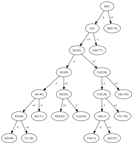
0(0) 1(0) -1 20(0.79) +1 2(0.02) +1 19(0.77) -1 3(0.09) -1 12(0.26) +1 4(0.48) -1 9(0.62) +1 5(0.68) +1 8(0.71) -1 6(0.68) -1 7(1.28) +1 10(0.82) +1 11(0.85) -1 13(0.26) -1 18(1.95) +1 14(0.3) -1 17(1.58) +1 15(0.3) -1 16(0.97) +1

Fig. 1. Example of a search tree formed by the OHRSA based STE in a scenario employing BPSK modulation,NRx = 2, M = 2, ∆ = 1,

L= 2,K= 2andNT x = 1and encountering Eb/N0 = 12dB. The exact received signal vectorx_{, the channel matrix}H_{and the transmitted} sequences_{are given in Equation (20). The labels indicate the search node} index, while the value of the costfunction of Equation (17) is given in brackets.

and

ˆ

s

(o)

M M SE

= [

−

0

.

11

−

0

.

61 0

.

10

−

0

.

12 0

.

69

−

1

.

01]

T

_.

(23)

Note that since both the system matrix and the transmitted signal

are real-valued, the imaginary part of the received sequence may be

omitted and the MMSE solution is also real-valued. The algorithm

commences at node 0 of Figure 1 by evaluating the cost function of

the hypothetical solutions

s

ˇ

(_No_s)

= ˇ

s

(6o)

associated with the ordered

channel matrix of Equation (21), according to Equation (17), which

yields

J

6

(ˇ

s

6

)

(o)

=

|u

(66o)

(ˇ

s

(o) 6

−

ˆ

s

(o) 6,M M SE

)

|

2

J

6

(ˇ

s

(6o)

= +1) =

|.

45

·

(+1 + 1

.

01)

|

2

= 0

.

79

J

6

(ˇ

s

(6o)

=

−

1) =

|.

45

·

(

−

1 + 1

.

01)

|

2

= 0

.

00

.

The two values

J

6

(ˇ

s

(6o)

)

can be seen at the second hierarchical

level of Figure 1 as nodes 1 and 20 together with the associated

hypothetical BPSK solutions indicated along the branches. Based

on the two cost function values seen within node 1 and 20 we

select node 1, since it has a value of

J

6

(ˇ

s

(6o)

=

−

1) = 0

.

0

, which

is the lower cost function value. The associated symbol value is

ˇ

s

(6o)

=

−

1

. In the next step of the algorithm we proceed from node

1 of Figure 1 by calculating the cost function of Equation (17) for

the next two potential values of

ˇ

s

(5o)

=

±

1

as follows:

a

5

=

6_j=6

u

(5oj)

·

(ˇ

s

(o)

j

−

s

ˆ

(o)

j,M M SE

)

=

0

.

06

·

(

−

1 + 1

.

01) = 0

.

00

J

5

([ˇ

s

(5o)

−

1]

T

₎

₌

_|a

5

+

u

(55o)

(ˇ

s

5

−

s

ˆ

(5o,M M SE)

)

|

2

J

5

([+1

−

1]

T

)

=

|

0

.

00 +

.

52

·

(+1

−

.

68)

|

2

= 0

.

02

J

5

([

−

1

−

1]

T

)

=

|

0

.

00 +

.

52

·

(

−

1

−

.

68)

|

2

= 0

.

77

.

The resultant two values for

J

5

(ˇ

s

(5o)

)

are associated with node 2

is node 2, where the associated symbol is

s

ˇ

(5o)

= +1

, which has

a lower cost function value than node 19.

The value of

ˇ

s

(o)

5

= [+1

−

1]

T

is now used for the calculation

of the cost function values of Equation (17) associated with

ˇ

s

(o) 4

.

The cost function values

J

4

(ˇ

s

(4o)

)

are illustrated at the fourth

hierarchical level of Figure 1 within node 3 and 12. Repeating this

procedure will result in the calculation of the cost function value

of

J

3

(ˇ

s

(3o)

)

provided within node 4 and 9 at the fifth hierarchical

level of Figure 1, the calculation of

J

2

(ˇ

s

(2o)

)

given in node 5 and

8 at the sixth hierarchical level of Figure 1 and finally

J

1

(ˇ

s

(1o)

)

[image:4.595.318.527.55.294.2]

given in node 6 and 7 at the seventh and last hierarchical level of

Figure 1.

Upon arriving at

J

1

(ˇ

s

(1o)

)

at the bottom of the graph, we have

calculated the first potential solution of our optimization problem

described by Equation (7), which is constituted by the left-most

branch of the search tree illustrated in Figure 1. This potential

solution is given by

ˇ

s

(o)

_{= [}

₋

_{1 + 1}

₋

₁

₋

_{1 + 1}

₋

_1]

T

_.

The recursive optimization continues from the bottom (node 6)

to the top of the tree of Figure 1 with the objective of finding

the specific branch terminating at the bottom of the search tree

(hierarchical level 6) while having the minimum costfunction

value. The symbol vector

s

_{associated with this branch constitutes}

the ML solution. Considering now the flipping of symbol

s

ˇ

(1o)

or

ˇ

s

(2o)

at hierarchical level 5 or 6 is not beneficial, since the cost

function associated with these changes would result in a higher

value, namely

1

.

28

and

0

.

71

, than the cost function of

0

.

68

at

node 6. Hence, if these tentative branches would be pursued to the

bottom of the tree, it would ultimately result in an increased cost

function value as a consequence of the ordering property outlined

in Equation (18).

When the recursive process initiated at node 6 arrives at node

3, however, it can be seen that changing the value of

s

ˇ

(₄o)

from

−

1

to

+1

results in a cost function value of 0.62 at node 3 which

is lower than the cost function value of 0.68 recorded at node 6.

Pursuing the path from node 9 further down the tree will however

again result in a cost function value that is higher than that of node

6. The corresponding branch is therefore not pursued further.

Returning to the most-left branch and changing the value of

ˇ

s

(₄o)

from

−

1

to

+1

, results in a cost function value of

0

.

26

,

which is lower than that of node 6 and the corresponding path is

therefore pursued further through nodes 13 and 14. Ultimately, this

results in two new branches through nodes 12 , 13, 14 and 15 as

well as 12, 13, 14 and 16 terminating at

ˇ

s

(o)

1

, which constitute

additional potential solutions for

s

(o)

_{. Pursuing this path from}

node 15 and 16 backwards, returning to the most-left branch and

moving recursively up to node 0 will result in no further branches

terminating at the bottom of the tree.

The desired solution is described by the specific branch

termi-nating at the bottom of the search tree and having the lowest cost

function value. Again, the associated symbol sequence is given by

ˇ

s

(o)

_{= [}

₋

₁

₋

₁

₋

_{1 + 1 + 1}

₋

_1]

T

_,

which can be obtained by tracing the branch back from node 15

to node 0. By contrast, the identically ordered MMSE solution is

given by

ˆ

s

(o)

M M SE

= [

−

1

−

1 + 1

−

1 + 1

−

1]

T

_.

The corresponding solutions for reversed ordering are then given

10

-5

10

-4

10

-3

10

-2

10

-1

10

0

0

5

10

15

20

BER

E

_b

/N

₀

[dB]

MMSE

OHRSA

Bayesian

MAP

Fig. 2. BER versusEb/N0 for a scenario supporting K = 1 user employingNT x= 2transmit AEs, a two-path equal-power block-fading

channel, a BS equipped withNRx = 2,M = 2,∆ = 1 and perfect

channel knowledge. BPSK modulation was considered.

by

ˇ

s

₌

_[

₋

₁

₋

₁

₋1 + 1

s_∆+1

+1

−

1]

T

ˆ

s

_{M M SE}

₌

_[

₋

₁

₋

₁

−1 −1

s_∆+1

+1 + 1]

T

,

which highlights the decision errors made by the MMSE detector.

The fact, that only a subset of the detector outputs is actually

of interest, namely the subvector

s

_∆+1

of

s

is a major

differ-ence between the OHRSA applied to the non-dispersive OFDM

subchannels in [1] and the wideband scenarios considered in this

treatise.

Following the procedure outlined in [1], the presented OHRSA

readily may be extended to account for complex-valued channel

matrices and higher order modulation schemes.

III-A. Results

In order to benchmark the proposed algorithm against

conven-tional DF-STEs proposed in the literature [6] a low-complexity

system consisting of

K

= 1

MS benefiting from

N

T x

= 2

number

of transmit antennas and communicating over a channel modelled

by two equal-power independently faded path. The signal was

assumed to be BPSK modulated and the BS employed

N

Rx

= 2

receive antennas as well as a DF aided STE in conjunction with

M

= 2

,

∆ = 1

and

N

= 1

. The fading envelope was assumed

to be constant during an entire transmission burst and no channel

coding was considered.

It can be seen from Figure 2 that the OHRSA indeed approaches

the performance bound constituted by the Bayesian DF-STE and

clearly outperforms the MMSE-based STE. The performance

dis-crepancy recorded in comparison to the Maximum A-Posteriori

(MAP) STE might be closed by considering a higher decision delay

in the STE.

[image:4.595.317.514.366.417.2]

10

-5

10

-4

10

-3

10

-2

10

-1

10

0

0

5

10

15

20

BER

E

_b

/N

₀

[dB]

K=1

K=2

K=3

K=4

MMSE

OHRSA

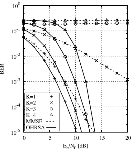
Fig. 3. BER versusEb/N0for a scenario supportingKnumber of users, each employingNT x = 2transmit AEs, a two-path equal-power

block-fading channel, a BS associated withNRx = 4,M = 2,∆ = 1and

perfect channel knowledge. 4QAM transmissions were considered.

10

1

10

2

10

3

10

4

10

5

10

6

10

7

10

8

10

9

10

10

1

2

3

4

No. Operations

No. MSs K

Search space

[image:5.595.66.278.55.294.2]

E

_b

/N

₀

=0dB

E

_b

/N

₀

=10dB

Fig. 4. The number of combined addition and multiplication operations required for the detection of a single bit by the system used for generating Figure 3.

number of MSs

K, while keeping the other system parameters

as

M

= 2

,

∆ = 1

and

N

= 1

. For this system the classic

Bayesian and MAP STE benchmarker are excessively complex,

hence only the OHRSA and the MMSE DF-STE are considered. In

Figure 3, which shows the attainable average BER versus

E

b

/N

0

performance for different numbers of MSs it can be observed,

that the OHRSA is capable of detecting all MSs’ signals, even

in heavily overloaded systems, whereas the MMSE STE falters.

The complexity required for the detection of the signals associated

with Figure 3 is shown in Figure 4. The curve labeled as ’Search

Space’ indicates the number of possible transmitted bit sequences

in the search space, whereas the other curves show the number

of operations (multiplications plus additions) required for the

evaluation of the cost function given in Equation (15) for the

detection of a single bit. The graph clearly indicates that the

complexity of the OHRSA is several magnitudes lower than the

complexity associated with a full ML detector. It can also be seen

that for a higher SNR the number of operations imposed is lower

than that required as lower SNRs.

IV. TRUNCATED SEARCH

In contrast to the application of the OHRSA for the detection

of the narrowband OFDM subcarriers, the detection of all symbols

in

s

_{is not required in the context of wideband systems, since we}

mentioned earlier that we are only interested in the detection of

the subvector

s

_∆+1

.

An attractive way of exploiting this phenomenon is to arrange

the columns of the channel matrix

H

_{not only according to the}

squared norm of the columns as suggested in [1], but also ensuring

that the columns of specific interest appear at the end of the ordered

channel matrix

H

(o)

_{. In other words, we try to ensure that the}

symbols associated with

s

_∆+1

_{appear at the top of the search tree}

and are therefore detected first.

The corresponding reordering scheme can be divided into two

steps as follows:

1) Set the last

Q

number of columns of the channel matrix

given by

(

H

₎

_i

_i

_∈

_[∆

_·

_Q

_{+ 1}

_,

_{(∆ + 1)}

_·

_Q

_]

to the columns arranged according to their power. This

ensures that the symbols of interest are detected first

ac-cording to the squared norm of the associated columns. The

associated symbols appear in the top section of the search

tree.

2) Set the remaining columns of the channel matrix ordered

ac-cording to the squared norm of the columns to the remaining

columns of the channel matrix, again, arranged according to

their squared norm.

From a physical point of view the columns with very low

squared norm may contribute very little to the final cost function

value. This yields, that the search tree is subject to a very fine

branching at its bottom levels which has little influence on the final

cost function value and increases the complexity because each of

these branches has to be evaluated. Due to the fact, that the desired

symbols appear now in the top section of the search tree, a certain

number of levels at the bottom of the tree might be neglected in

order to avoid the evaluation of the cost function associated with

the fine branching.

The recursive cost function of Equation (17) can then be

rewritten as

J

i

(ˇ

s

i

) =

J

i+1

(

s

i+1

) +

φ

(

s

i

)

, i

=

N

s

−

1

, . . . , N

trunc

+ 1

,

(24)

where

N

trunc

indicates the number of layers of the search tree

that have been discarded. Note however that truncation will always

result in performance degradation, because even though we are not

interested in the final decision concerning some of the symbols,

they still mildly influence the channel’s output vector

x

_{and the}

cost function as it becomes explicit from Equation (9). Under

certain circumstances, however, when the power associated with

these symbols is very low (the associated column of the channel

matrix has a low squared norm), their influence becomes marginal

and might be neglected.

IV-A. Results

The effect of truncating the search tree has first been investigated

for the same system as the one studied in Figure 3. The number

of operations shown in Table I was recorded for

E

b

/N

0

=10 dB

[image:5.595.64.279.353.489.2]

K= 1 K= 2 K= 3 Ntrunc= 2 Ntrunc= 4 Ntrunc= 4

Full 44 77 353

Trunc. 27 44 122

TABLE I

NUMBER OF OPERATIONS REQUIRED FOR THE DETECTION OF ONE BIT

ATEb/N0=10DBASSOCIATED WITH THE SYSTEM USED FOR GENERATINGFIGURE3IF TRUNCATION IS USED.

K= 1 K= 2 Ntrunc= 4 Ntrunc= 8

Full 254 7.1_·104

Trunc. 60 193

TABLE II

NUMBER OF OPERATIONS REQUIRED FOR THE DETECTION OF ONE BIT

ATEb/N0=10DBASSOCIATED WITH THE SYSTEM USED FOR GENERATINGFIGURE5IF TRUNCATION IS USED.

Due to lack of space the corresponding BER curves are not

included. It is worth mentioning that the two-path equal-power

model channel may be considered to correspond to the

worst-case scenario, because the difference in squared norm between

the columns of the channel matrix associated with the desired and

the undesired symbols is not dramatic.

Let us therefore consider a more optimistic propagation scenario

having four equal-power paths and a DF-STE associated with

M

= 4

,

∆ = 3

,

N

= 3

and

N

Rx

= 4

receive antennas. Each user

employed

N

T x

= 2

transmit AEs and the channel code employed

was a half-rate punctured turbo-code [4] which was operating on

the hard-decision output of the DF-STE. In Table II the complexity

reduction achieved as a benefit of the above-mentioned truncation

procedure is summarized and the associated BER performance is

shown in Figure 5. It can be observed that the truncation technique

in this scenario provides a significant complexity reduction which

is of several orders of magnitudes attained at the cost of little

performance degradation. The associated high number of

opera-tions required for the conventional OHRSA assisted DF-STE is

due to the fact that the low power associated with some columns

of the channel matrix results in numerous extra branches at the

bottom of the search tree all of which have to be considered by

the algorithm. It is exactly this set of low-power branches, which

can be truncated without any significant loss of performance. The

higher difference in squared norm compared to the two-path system

is caused by the Toeplitz structure of the channel matrix

H

_{, which}

is the characteristic of STEs.

V. CONCLUSION

A novel DF aided reduced complexity ML detector has been

proposed for employment in single-carrier wideband scenarios

. The detector was based on the recently contrived OHRSA

algorithm [1], which has been further developed for employment

in a single-carrier STE. It was shown that the proposed receiver

struture substantially outperforms the linear benchmarker based on

the MMSE criterion. Furthermore, a complexity reduction scheme

based on truncating the search tree has been proposed, which

accommodates the specific properties of the associated propagation

channel. The proposed modification of the OHRSA complements

10

-5

10

-4

10

-3

10

-2

10

-1

10

0

0

1

2

3

4

5

6

7

8

BER

[image:6.595.72.274.56.116.2]

E

_b

/N

₀

[dB]

K=2, Trunc

K=2, Full

K=1, Trunc

K=1, Full

Fig. 5. BER versus Eb/N0 for a scenario supporting K number of users, each employingNT x = 2transmit AEs, a four-path equal-power

block-fading channel, a BS associated withNRx= 4,M = 4,∆ = 3

and perfect channel knowledge. 4QAM transmissions and a half-rate turbo code were considered.

the DF-STE in a sense, that the symbols associated with the

post-cursor of the CIR can be combatted by the DF structure, whereas

the low-power pre-cursor of the CIR might be neglected for the

sake of reducing the complexity of the OHRSA aided STE by

truncating the search tree.

VI. REFERENCES

[1] J. Akhtman and L. Hanzo, “Reduced-complexity

maximum-likelihood detection in multiple-antenna-aided multicarrier

sys-tems,” in

Proceedings of 5th Int’l Workshop on Multi-Carrier

Spread Spectrum (in press)

, (Oberpfaffenhofen, Germany),

2005.

[2] L. Hanzo, M. M¨unster, B. Choi, and T. Keller,

OFDM and

MC-CDMA for Broadcasting Multi-User Communications, WLANs

and Broadcasting

. John Wiley and IEEE Press, July 2003.

[3] B. Hassibi and H. Vikalo, “On the sphere-decoding algorithm

I. Expected complexity,”

Signal Processing, IEEE Transactions

on [see also Acoustics, Speech, and Signal Processing, IEEE

Transactions on]

, vol. 53, pp. 2806–2818, 2005.

[4] L. Hanzo, C. H. Wong, and M. S. Yee,

Adaptive Wireless

Transceivers: Turbo-Coded, Turbo-Equalized and Space-Time

Coded TDMA, CDMA, and OFDM Systems

. John Wiley and

IEEE Press, Feb. 2002.

[5] S. Chen, B. Mulgrew, E.-S. Chng, and G. J. Gibson, “Space

translation properties and the minimum-BER linear-combiner

DFE,”

IEE Proceedings on Communications

, vol. 145,

pp. 316–322, October 1998.