Transfer matrix analysis of the elastostatics of one dimensional repetitive structures

Transfer matrix analysis of the elastostatics of

one-dimensional repetitive structures

BY N. G. STEPHEN*

Mechanical Engineering, School of Engineering Sciences, University of Southampton, Highfield, Southampton SO17 1BJ, UK

Transfer matrices are used widely for the dynamic analysis of engineering structures, increasingly so for static analysis, and are particularly useful in the treatment of repetitive structures for which, in general, the behaviour of a complete structure can be determined through the analysis of a single repeating cell, together with boundary conditions if the structure is not of infinite extent. For elastostatic analyses, non-unity eigenvalues of the transfer matrix of a repeating cell are the rates of decay of self-equilibrated loading, as anticipated by Saint-Venant’s principle. Multiple unity eigenvalues pertain to the transmission of load, e.g. tension, or bending moment, and equivalent (homogenized) continuum properties, such as cross-sectional area, second moment of area and Poisson’s ratio, can be determined from the associated eigen- and principal vectors. Various disparate results, the majority new, others drawn from diverse sources, are presented. These include calculation of principal vectors using the Moore– Penrose inverse, bi- and symplectic orthogonality and relationship with the reciprocal theorem, restrictions on complex unity eigenvalues, effect of cell left-to-right symmetry on both the stiffness and transfer matrices, eigenvalue veering in the absence of translational symmetry and limitations on possible Jordan canonical forms. It is shown that only a repeating unity eigenvalue can lead to a non-trivial Jordan block form, so degenerate decay modes cannot exist. The present elastostatic analysis complements Langley’s (Langley 1996 Proc. R. Soc. A 452, 1631–1648) transfer matrix analysis of wave motion energetics.

Keywords: transfer; symplectic; matrix; elastostatic; pseudo-inverse; Jordan canonical form

1. Introduction

Repetitive (or periodic) structures are analysed most efficiently when such periodicity is taken into account. A typical approach (Langley 1996) relates a state vector of displacement and force components on either side of a generic repeating cell by a transfer matrix, G, which may be determined from the stiffness matrixK, although discrete displacement field (Karpovet al. 2002a) and discrete Fourier transform (Karpovet al. 2002b) formulations are also possible. An eigenvector of the transfer matrix describes a pattern of displacement and force components which is unique to within a scalar multiplier; translational

Published online28 February 2006

*[email protected]

symmetry demands that this pattern is preserved as one moves from the left-hand to the right-left-hand side of the cell, allowing one to write sRZlsL; this leads to the standard eigenvalue problem lsLZGsL, orðGKlIÞs_LZ0. For dynamic problems, this is an application of Bloch’s theorem (seeBrillouin 1953), and leads to an eigenvalue problem for the propagation constants or, equivalently, the natural frequencies; the approach is highly developed and has been applied to both one-dimensional (beam-like) and two-dimensional (plate-like) problems (Mead 1970, 1996; Meirowitz & Engels 1977; Yong & Lin 1989a,b; Zhong & Williams 1992, 1995;Langley 1996). The theory is less well developed for static analysis, but has been applied to one-dimensional prismatic planar (Stephen & Wang 1996a), asymmetric and pre-twisted (Stephen & Zhang 2004, 2006) and curved repetitive structures (Stephen & Ghosh 2005).

This paper is concerned largely with the static problem, and presents numerous results concerning the eigenanalysis of a (real) transfer matrix G; some of these results are not new, but are drawn from diverse references in order to provide a convenient resource. As a consequence of the symmetry of the stiffness matrixK, the transfer matrix has the property of being symplectic (Pease 1965), so its eigenvalues occur as reciprocals, and fall into five possible classes (Meyer & Hall 1991):

(i) The real unity eigenvaluelZ1, which must occur an even number of times;

the inverse is a repeat.

(ii) The negative real unity eigenvaluelZK1, which must occur an even number of times; again the inverse is a repeat.

(iii) The real non-unity eigenvalues occur as a pairlandlK1_.

(iv) The complex unity eigenvalues occur as a unitary pairlZeiaandlZeKia_; the inverse is simultaneously the complex conjugate.

(v) The general complex eigenvalues occur as a quartet of reciprocals and complex conjugates, that is lZaCib, lZaKib, lZðaCibÞK1 and lZ ðaKibÞK1are all, as an ensemble, possible eigenvalues.

A consequence of the above is that the determinant of a symplectic matrix is equal toC1. Suppose that lis an eigenvalue having multiplicity k, then lK1 is an eigenvalue also having multiplicityk; thus, the Jordan blocks corresponding to l

and lK1 _{have the same structure. The group of real symplectic matrices of size} 2n!2n, denoted Spðn;RÞ, is the fundamental group underlying classical mechanics yet, according to Abraham & Marsden (1978), ‘very little application of its structure seems to have been made beyond these elementary eigenvalue properties’. Symplectic matrices have the property of preserving Hamiltonian structure, and are often employed as similarity matrices within the field of Floquet (periodic) dynamic systems, such as one finds in the field of celestial mechanics (Meyer & Hall 1991); they also find application within optimal control engineering (Stengel 1986), and time-series analysis (Aoki 1987). Their introduction into the field of solid mechanics is largely due to Zhong et al. (1992), Zhong & Williams (1992,1995) andZhong (1995).

couplings between the various modes; for example, a shearing force is inevitably coupled to a bending moment. Moreover, equivalent continuum (homogenized) properties of the reticulated structure may be calculated.

Studies by the present author and co-workers have previously concentrated on pin-jointed repetitive structures; this choice was made because the finite-element analysis (FEA) of such structures may be regarded as exact; in turn, predictions from the eigenanalysis can be verified by comparison with what may be regarded as exact FEA results. This does not imply that pin-jointed structures are not of interest in their own right; indeed, the removal of members from such a structure can reduce it to a mechanism, which in turn allows its transportation in a very compact form, an attribute likely to find favour in aerospace application. Here we record the effect of rigid- rather than pin-jointing; the continuum properties are virtually unchanged, and one has new decay modes associated with self-equilibrated moments applied at the nodes. Repetitive structures are not limited to frameworks, or lattice structures; a continuum structure such as a metre rule would be perfectly repetitive were it not for the progressive numbering along its length—each centimetre of rule is identical to that preceding and following. Thus, Stephen & Wang (1996b) have developed a hybrid finite element/transfer matrix

Table 1. Notation.

a,A,A constant, cross-sectional area, matrix

b,b,B constant, column vector, similarity matrix

d,d component of, nodal displacement vector

e,E eigenvector, Young’s modulus

F,F component of, nodal force vector

G,G transfer matrix, shear modulus

H Hamiltonian system matrix

I,I identity matrix, second moment of area

J,Jm Jordan canonical form, metric

L left, length

K,k stiffness matrix, dimension of Jordan block, eigenvalue

M nodal moment component

N,n,N nilpotent matrix, index, number of cells, nodal moment component

p,p component of, nodal force vector, principal vector

R,R,R right, reflection matrix, real numbers

s,S state vector, real symmetric matrix

V similarity matrix of eigen- and principal vectors

x,y,z Cartesian coordinates

x vector

X,Y (right) eigenvectors ofGandGT

a arbitrary angle

b arbitrary multiple

l eigenvalue

k shear coefficient (in Timoshenko beam theory)

n Poisson’s ratio

q arbitrary angle

gld greatest linear dimension JCF Jordan canonical form

method that allows one to calculate the Saint-Venant decay rates of self-equilibrated loading for rods or beams of general cross-section. On the other hand, if there is no discretization of the continuum, then the symplectic transfer matrix

Gis replaced by a Hamiltonian system matrixH, within a relationship of the form ds

dxZHs; ð1:1Þ

where the state vector s consists of the displacement components and the cross-sectional stress components. This state-space approach to theTheory of Elasticity

was developed by Zhong (1995), and an exposition was presented recently by Stephen (2004) for the elastostatics of a prismatic rod or beam, where it was also shown that only a repeating zero eigenvalue can lead to a non-trivial Jordan block form.

The present paper may be seen as complementary to a recent analysis of wave motion energetics using transfer matrices (Langley 1996). However, besides some introductory definitions and results, the focus is quite different; the latter specifically excludes issues relating to principal eigenvectors attendant upon the multiple (unity) eigenvalues, which is a particular feature of the static analysis. Moreover, dynamic analyses typically assume the structure to be of infinite extent, which avoids issues relating to boundary conditions. For the static case, while general results may be gleaned from a single cell, boundary conditions at both ends of the structure must be taken into account in order to provide a complete solution to any particular problem. The introductory material includes previously known results, including the reciprocal eigenvalue properties as a consequence of the symplectic nature of the transfer matrix, bi- and symplectic orthogonality and the relationship with the Betti–Maxwell reciprocal theorem, and the impossibility of complex unity eigenvalues for prismatic repetitive structures. The Moore–Penrose pseudo-inverse is introduced as a rational approach to the computation of principal vectors associated with the multiple unity eigenvalues. Employing a strain energy argument, it is shown that only the eigenvalues lZG1 can give rise to a non-trivial JCF, at least for the prismatic structure. An example of a structure for which the transfer matrix has repeating negative unity eigenvalue is one possessing a scissor-like mechanism, and this possibility can be gleaned through simple arguments regarding the dimension of the transfer matrix. A planar structure, previously treated as pin-jointed, is reconsidered as rigid-jointed; the additional rotational nodal degrees of freedom give rise to new Saint-Venant decay modes—the number of transmission modes associated with unity eigenvalues is fixed—while the equivalent continuum properties are practically unaffected. This confirms the practice of treating real, rigid-jointed structures as pin-jointed, at least for small deflection elastic analysis. A variety of relationships between partitions of both the stiffness and transfer matrices results are presented for a cell possessing left-to-right symmetry. On the other hand, lack of symmetry implies less restriction, and one has splitting of unity eigenvalues for a tapered cell that lacks translational symmetry.

2. Transfer matrix formulation

Stephen & Wang (1996a): the Young modulus of each member is

EZ200!109N=m2, horizontal and vertical members are of length LZ1 m and have (circular) cross-sectional area_ffiffiffi AZ1 cm2; the diagonal members have length

2 p

m and cross-sectional area 0:5 cm2. However, since vertical members are regarded as being shared between adjacent cells, the repeating single cell must have vertical members with one-half stiffness; for the pin-jointed structure, this just requires that the cross-sectional areas should be A/2. For the rigid-jointed structure, the members can also carry bending moment, so it is also required that the bending stiffness and, hence, the second moment of area should be halved.

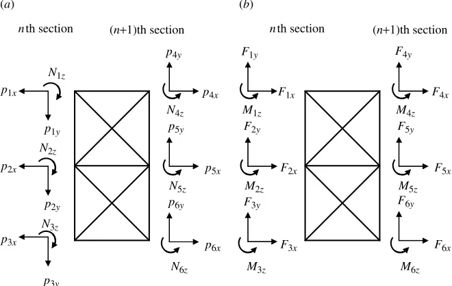
A typical cell located between thenth and (nC1)th sections of the structure in figure 1is shown infigure 2. Letpn anddn denote the generalized nodal force and

displacement vectors, respectively, associated with the nth section; the state vectors at the section nth and ðnC1Þth sections are then s_nZ½dT_n pT_nT and snC1Z½d

T

nC1 p

T nC1

T

, and they are related by the transfer matrixGthrough the equation

snC1ZGsn; ð2:1Þ

1st 2nd nth cell Nth

x y

Figure 1. Rigid- or pin-jointed planar framework, fixed at left-hand end and subject to tensile force at the right; the length of the truss is equal to the number of the cells,N.

nth section (n+1)th section nth section (n+1)th section

(a) (b)

p_1x

p_1y N_1z

p_2x

p_2y N_2z

p_3x

p_3y N_3z

p_4x p_4y

N_4z

p_5x p_5y

N_5z

p_6x p_6y

N_6z

F_1x F_1y

M_1z

F_2x F_2y

M_2z

F_3x F_3y

M_3z

F_4x F_4y

M_4z

F_5x F_5y

M_5z

F_6x F_6y

M_6z

or in partitioned form

dnC1

pnC1

Z

Gdd Gdp Gpd Gpp

" #

dn pn

: ð2:2Þ

Two consecutive state vectors are also related by a scalarl as

snC1Zlsn; ð2:3Þ

this is the static equivalent of an application of Bloch’s theorem for systems possessing translational symmetry. Substitution of the above into equation (2.1) leads directly to the standard eigenproblem

½GKlIs_nZ0; ð2:4Þ

where I is the identity matrix of the appropriate size. The eigenvalues of the transfer matrix describe how associated eigenvectors scale as one moves from one nodal section to the next. A unity eigenvalue implies that it is transmitted unchanged, while a non-unity eigenvalue jlj!1 implies that the nodal displacements and forces decay as one moves from cell to cell, left-to-right; the reciprocal, jlK1_{jO1 represents an increase from left-to-right, hence a decay from} right-to-left.

The transfer matrix G is obtained from the stiffness matrix K of the single repeating cell; referring tofigure 2b, the generalized force and displacement vectors

F and d are related by the stiffness matrix equation FZKd, or in partitioned

form

Fn FnC1 " #

Z

KLL KLR KRL KRR

" #

dn dnC1 " #

: ð2:5Þ

Transfer matrix analysis employs the sign conventions of theTheory of Elasticity, so set FnZKp_n, F_nC1Zp_nC1, and substitute into equation (2.5), expand and rearrange to give

dnC1

pnC1

ZG dn pn

; ð2:6Þ

when the transfer matrix G becomes

G_Z KK

K1

LRKLL KKK_LR1 KRLKKRRKKLR1KLL KKRRKKLR1

" #

: ð2:7Þ

Having performed the eigenanalysis, a similarity matrix Vconsisting of all eigen-and principal vectors including both decay eigen-and transmission modes can be constructed and this transforms the transfer matrix Gto JCF according to

VK1

GV ZJ; ð2:8Þ

where J is the JCF. The multiple unity eigenvalue typically appears in two or more distinct Jordan blocks, so the transfer matrix G is both defective and

derogatory. Not only does the JCF reveals the coupling between the various modes, e.g. the shearing force principal vector is coupled to the bending moment vector, it also allows one to calculate powers of the transfer matrixGin the most efficient and accurate manner; suppose one knows the applied state vectors(0) on the zerothleft-hand end of the structure in figure 1, the state vector on the right-hand side of this first cell is given by

and the state vector on the right-hand side of the nth cell is then

sðnÞZGnsð0Þ: ð2:10Þ

Powers of the transfer matrix (the cumulative transfer matrix) are evaluated according to

Gn_ZðVJVK1

Þn _ZðVJVK1

ÞðVJVK1

Þ_.ðVJVK1

Þ_ZV JnVK1

: ð2:11Þ Moreover, thenth power of the JCF simply requires evaluation of thenth power of the diagonal elements, although for the non-trivial Jordan blocks, a more involved treatment is required. LetJi be a Jordan block pertaining to eigenvalueli, having

dimensionk!k, written as

Ji Z

li 1 1 1

li 1 li 2 6 6 6 6 4 3 7 7 7 7

5ZliICNi; ð2:12Þ

where Ni is the nilpotent matrix

NiZ

0 1 1 1 0 1 0 2 6 6 6 6 4 3 7 7 7 7

5: ð2:13Þ

Thekth power of the nilpotent matrix is zero, so the binomial expansion ofJniZ

ðliICN_iÞn has a finite number of terms as

ðliICN_iÞn_Zln_iIC

n

1 !

lnK1

i NiC

n

2 !

lnK2

i N

2

i C_/C

n kK1

!

lnKkC1

i N

kK1

i ;

ð2:14Þ since higher powers ofNiare zero; in the above, the binomial coefficients are given by

n b

!

ZnðnK1ÞðnK2Þ/ðnKbC1Þ

b! : ð2:15Þ

Thenth power of the Jordan block becomes

Jni Z

lni nlniK1

nðnK1Þ

2 l

nK2

i /

0 lni nlniK1 /

0 0 lni /

/ / / / 2 6 6 6 6 6 6 6 6 6 4 3 7 7 7 7 7 7 7 7 7 5

: ð2:16Þ

Expression (2.10) becomes

sðnÞ_ZV JnVK1

sð0Þ; ð2:17Þ

but before it can be applied one requires complete knowledge of the state vector

tofigure 1, one knows the force vectorpN at theNth nodal cross-section, but not

the displacement components. On the other hand, at the fully fixed left-hand end, one knows the displacement vector d0(equal to a zero column) but not the force

vector p0 which, besides the reaction to the tensile force, must contain

self-equilibrating load sufficient to suppress Poisson’s ratio contraction effects. The state vectors at either end are related by a cumulative transfer matrix as

sðNÞ_ZV JNVK1

sð0Þ; ð2:18Þ

or in more detail

dN pN

Z

GddN GdpN GpdN GppN

" #

d0 p0

; ð2:19Þ

where GddN; GdpN; GpdN andGppN are square partitions of V JNVK1. With the

exception ofGpdN, these partitions are invertible; partitionGpdN must be singular,

as the displacement vector d0 cannot be calculated from knowledge of the force vectors at each end—one can always add rigid body displacements or rotations. From the second row, one hasp0ZGKppN1 pNKGK_ppN1 GpdNd0, and substituting this into the second row yieldsdNZðGddNKG_dpNGK_ppN1 G_pdNÞd₀CG_dpNGK_ppN1 p_N. One now has complete knowledge of the state vectors at each end. This process may be extended to other end conditions: for example, suppose that the uppermost support at the left-hand of the structure,figure 1, is removed; now only four of the elements of the vector d0 are equal to zero, but two of the elements of p0 would now also be equal to zero. Thus, the state vector sð0Þ can be re-ordered as six known (subscriptk) and six unknown (subscriptu) components as

dN pN

Z

GdkN GduN GpkN GpuN

" #

skð0Þ

suð0Þ

" #

; ð2:20Þ

with rows and columns of the complete structure transfer matrix being rearranged accordingly; the above manipulations are now applied to equation (2.20) rather than (2.19).

3. Calculation of principal vectors: the pseudo-inverse

Numerical determination of a non-trivial JCF of a matrix is generally unstable, and is possible only if the matrix elements are known exactly, for example, as integers or integer fractions, or if the repeating eigenvalues are known exactly, for example, on physical grounds (Kailath 1980); fortunately, the latter is true for the multiple real and complex unity eigenvalues that arise in the present approach. The majority of textbooks (e.g. Ogata 1990) suggest that one should start by calculating the principal vector of highest grade, that is, for a chain of k eigen- and principal vectors, one should first determine the principal vectorpk from the equation

½GKlIkp_kZ0; ð3:1Þ

rotation; essentially, this is a trade between choosing arbitrary elements of the principal vector of highest grade just once (but with no guarantee that this will lead to the simplest eigenvector) and making a simple choice several times over as one works along the chain toward the highest grade principal vector. The Moore– Penrose or pseudo-inverse of a rank-deficient matrix removes this element of choice and assigns values to the arbitrary elements in a rational manner.

Consider the matrix equation AxZb; the most common application of the

pseudo-inverse is when one has more equations than unknowns, which is typical of linear regression of experimental data and there is no solution in the classical sense. MatrixAhas more rows than columns, so is obviously not invertible. Pre-multiply byAT to give

ATAxZATb: ð3:2Þ

Matrix ATA is now square and may be inverted to give xZðATAÞK1ATb, or xZALMb, where the left pseudo-inverse is ALMZðATAÞK1AT. This solution is

often denoted as x8 and has the property of minimizing the norm kAx8Kbk. On the other hand, whenAhas more columns than rows (rank deficient), which is typical of the situation when calculating eigen- and principal vectors, there are an infinite number of solutions (recall that an eigenvector is a unique pattern which may be multiplied by a scalar to give an equally valid eigenvector; similarly, one may add an arbitrary multiple of a generating eigenvector to a principal vector and it is still a principal vector). Now, one requires therightpseudo-inverse defined as ARM_ZATðAATÞK1_{, for which}

AARM_ZAATðAATÞK1

ZI; ð3:3Þ

the above expression (which is equal to a conforming identity matrix) is nowshoe

-hornedinto equation (3.2) to give

ATAx8_ZAT AATðAATÞK1 |fflfflfflfflfflfflfflfflfflfflffl{zfflfflfflfflfflfflfflfflfflfflffl}

I

!

b: ð3:4Þ

As with the left pseudo-inverse, now pre-multiply by ðATAÞK1

to give

x8ZATðAATÞK1b

|fflfflfflfflfflfflfflfflfflffl{zfflfflfflfflfflfflfflfflfflffl}

ARM

: ð3:5Þ

Of the infinite number of solutions, the above is that which has minimum normkx8k, i.e. x8 is closest to the origin. Physically, one is adding multiples of the generating eigenvector (the rigid body displacement), such that the principal vector has displacements that are, on average, closest to the origin. For the symmetric cell shown in figure 1, when calculating the principal vector describing tension, the minimum norm solution provided by the pseudo-inverse is such that the axial (x-direction) displacement is zero, and the average of nodal displacements in they-direction is also zero. Node 2 has zero vertical displacement, while the Poisson ratio effects on nodes 1 and 3 are equal and opposite; this is exactly what one would have chosen.

4. Rigid- versus pin-jointing

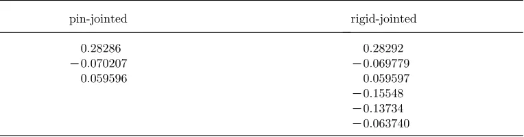
number of transmission modes having unity eigenvalue is unchanged at six, the immediate effect of rigid-jointing is to double the number of (left-to-right) Saint-Venant decay modes from three to six, as shown in table 2, together with their reciprocals which are not shown.

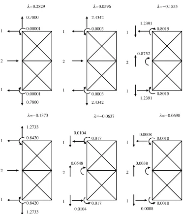
Rigid jointing has negligible effect on the three left-to-right decay rates of the pin-jointed cell; the main effect is the introduction of three new decay modes, two of which (l_ZK0.15548 and K0.13734) decay at approximately twice the rate of the dominant (slowest rate of decay) mode (l_Z0.28292); the minus sign indicates that the decay is oscillatory from cell to cell. For the pin-jointed structure, the decay eigenvectors consist of nodal forces which self-equilibrate in the x- and y -directions, it being impossible to apply a moment at a pin-joint. With rigid-joints, these modes now have a very small additional self-equilibrated moment—indeed, just sufficient that the displacement components of the eigenvector should decay with the specified eigenvalue. The new decay modes still have self-equilibrated force loading in the x- and y-directions, but with the addition of comparatively large self-equilibrating nodal moments. The force and moment components of the left-to-right decay eigenvectors are shown in figure 3.

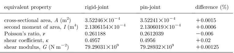
A comparison of the equivalent continuum properties is shown in table 3. As might be expected, the effect of rigid-jointing is to increase all of the equivalent stiffness’—note that a decrease in Poisson’s ratio is equivalent to an increase in the shear modulusGsince the Young modulusEis regarded as fixed; however, these increases are quite negligible.

5. Symplectic nature of the transfer matrix and consequences

The (2n!2n) transfer matrix Gsatisfies the relationship

GTJmGZJm; ð5:1Þ

whereJm is the metric matrix

JmZ

0 I

KI 0 " #

;

with JTmZJKm1ZKJ_m, and I is the (n!n) identity matrix. This relationship depends solely on the symmetry of the stiffness matrix K, and can be verified by direct substitution from equation (2.7). Moreover, the symplectic relationship, equation (5.1), requires that partitions of the transfer matrix satisfy the

Table 2. Saint-Venant decay factors.

pin-jointed rigid-jointed

0.28286 0.28292

K0.070207 K0.069779

0.059596 0.059597

relationships

GTddGpdZðG T ddGpdÞ

T

; ð5:2aÞ

GTdpGppZðG T dpGppÞ

T

; ð5:2bÞ

GTddGppKGT_pdG_dpZI: ð5:2cÞ The symplectic relationship GTJmGZJm can be rearranged to give JK1

mGTJmZGK1; thus, the inverse of G is similar to the transpose of G, which in turn has the same eigenvalues asG. Thus, the eigenvalues occur as reciprocals. Alternatively, one may employ a theorem by Taussky & Zassenhaus (1959): for

1

2

1

0.7800

0.7800

1

2

1

2.4342

2.4342

l=0.2829 l=0.0596

1

2

1

1.2391

1.2391

l=−0.1555

1

2

1

1.2733

1.2733

l=−0.1373

1

2

1

1

2

1 0.0104

0.0104

0.0008

0.0008

l=−0.0637 l=−0.0698

0.00001

0.00001

0.0003

0.0003

0.8015

0.8015 0.8752

0.8420

0.8420

0.0010

0.0010 0.0038

0.017

0.017 0.0548

every real square matrix G, there exists a (non-unique) non-singular real symmetric matrixS, such thatGTZSK1_{GS; that is,Gis similar to its transpose.} Combining the above two relationships yields

ðSJmÞK1GðSJmÞZGK1; ð5:3Þ

thus, the inverse of G is similar to G, and not only do the eigenvalues occur as reciprocals, but G and the inverse of G also have the same JCF. Thus, the multiplicity of an eigenvalue and its inverse must be the same, and any non-trivial Jordan block structure must be the same for an eigenvalue and its inverse. Moreover, from equation (2.8) one has GZVJVK1 _{and its inverse}

GK1

ZVK1_JK1_{V, and substituting into equation (5.3) yields} ðVK1

SJmVÞK1JðVK1SJmVÞZJK1: ð5:4Þ Thus, the JCF and its inverse are similar, and one may conclude that the JCF of

JK1 _{is nothing other than J. The structure of the similarity matrix B}

b VK1_SJ

mV may be determined (Gantmacher 1959) as follows: first re-arrange equation (5.4) as JBKBJK1Z0, or in block form

J1 0 /

0 J2

« ₁

2 6 4

3 7 5

B11 B12 / B21 B22

« ₁

2 6 4

3 7 5K

B11 B12 / B21 B22

« ₁

2 6 4

3 7 5

JK1

1 0 /

0 JK1

2

« ₁

2 6 6 4

3 7 7 5Z0;

ð5:5Þ where Bij is a (not necessarily square) block decomposition of B, compatible (conforming) with the size of the Jordan blocks. Each of the Jordan blocks may be written as JiZliICNi, whereNi is nilpotent; the inverse of the block, according to equation (2.16), may be written asJK1

i ZlKi1ICNi, whereNi is also

nilpotent. Equation (5.5) is then broken up and rearranged as

ðliKlKj1ÞBijZBijNjKNiBij: ð5:6Þ Now for ðliKlK_j1Þ_s0, one may multiply by ðl_iKlK_j1Þ, and substitute from equation (5.6) to give

ðliKlK_j1Þ2B_ijZB_ijN 2

jK2N_iB_ijN_jCN2_iB_ij: ð5:7Þ

This process may be repeated a sufficient number of times, when the right-hand side eventually becomes equal to zero because of the nilpotency of Ni andNj.

Thus, one concludes that ðliKlK_j1ÞBijZ0, and hence

BijZ0; forðliKlKj1Þs0: ð5:8Þ Table 3. Effect of nodal joining on equivalent continuum stiffness properties.

equivalent property rigid-joint pin-joint difference (%)

cross-sectional area,A(m2) 3.52246!10K4

3.52241!10K4

C0.0015 second moment of area,I(m4) 2.1306154!10K4 _2.1306019!10K4 _C0.0006 Poisson’s ratio,n 0.261188 0.2612039 K0.006

shear coefficient,k 0.4957 0.4956 C0.02

shear modulus,G(N mK2

For ðliKlK_j1Þ_Z0, orl_il_jZ1, one has

BijNj KNiBijZ0 ð5:9Þ

for a non-trivial block. This may be solved according to the structure of the nilpotent matrices, and several of the elements of the Bij will be arbitrary. The

process is best illustrated by a simple example: assume a 6!6 JCF

J1 J2

l2

lK1

2 2 6 6 6 6 4 3 7 7 7 7 5Z

l1 1 l1

lK1

1 1

lK1

1

l2

lK1

2 2 6 6 6 6 6 6 6 6 6 6 6 4 3 7 7 7 7 7 7 7 7 7 7 7 5

; ð5:10Þ

where the remaining elements are zero. We thus have two Jordan blocks and two trivial diagonal blocks. The block decomposition of B has four 2!2 blocks ðB11; B12; B21andB22Þ, four 2!1 blocks ðB₁₃; B₁₄; B₂₃andB₂₄Þ, four 1!2 blocksðB31; B32; B41andB42Þ; the remaining blocks are scalar. Immediately, on account of equation (5.8), the only non-zero blocks are B12; B21 and the scalar blocks B34 and B43 For a block such as B12, equation (5.9) becomes B12N2KN₁B_12Z0, or explicitly

b1 b2

b3 b4 " #

0 KlK₁2

0 0 " # K 0 1 0 0 " #

b1 b2

b3 b4 " #

Z0; ð5:11Þ

expanding gives

Kb3 Kb4KlK₁2b1 0 KlK₁2b₃

" #

Z0; ð5:12Þ

from which one hasb3Z0 and b4ZKlK₁2b₁, and the block takes the form

B12Z

b1 b2

0 KlK₁2b₁

" #

: ð5:13Þ

The scalar blocks are arbitrary, and the similarity matrix takes the form

B_Z

0 0 b1 b2 0 0

0 0 0 KlK₁2b1 0 0

b3 b4 0 0 0 0

0 Kl2₁b₃ 0 0 0 0

0 0 0 0 0 b5

0 0 0 0 b6 0

2 6 6 6 6 6 6 6 6 6 6 4 3 7 7 7 7 7 7 7 7 7 7 5

: ð5:14Þ

6. Bi- and symplectic orthogonality and the reciprocal theorem

Since the transfer matrix G is not symmetric, one would normally employ bi-orthogonality as the means of modal decomposition of an arbitrary state vector. LetXi be a (right) eigenvector ofG associated with the eigenvalueli, such that

GXiZliXi; ð6:1Þ

letYj be a (right) eigenvector ofGT associated with the eigenvaluelj, such that

GTYj ZljYj: ð6:2Þ

Pre-multiply equation (6.1) by YTj to give YTj GXiZliY

T

j Xi; ð6:3Þ

transpose equation (6.2), and post-multiply by Xi to give

YTj GXiZljYTj Xi: ð6:4Þ

Subtraction gives

ðliKljÞY T

j XiZ0; ð6:5Þ

and the bi-orthogonality relationship

YTj XiZ0; forlislj: ð6:6Þ

In principle, the disadvantage of this approach is the need to perform a second eigenanalysis of the transpose of G, although in practice one needs only to compute the eigen- and principal vectors, as the eigenvalues ofGTare the same as those of G. Instead, symplectic orthogonality is determined as follows: transpose equation (6.1) to give

XTi GTZliXTi : ð6:7Þ

Post-multiply byJmGXj to give XTi G

T

JmGXj ZliX T

i JmGXj: ð6:8Þ

NowGTJmGZJmandGXjZljXj, and substituting these expressions into (6.8)

yields

ð1Kl_il_jÞXT_i J_mX_{j Z}0: ð6:9Þ

Thus, an eigenvector is symplectic adjoint orthogonal to all vectors, including itself, but excluding the vector(s) associated with its reciprocal eigenvalue.

The two orthogonality relationships are clearly related, as follows: Yj is the

(right) eigenvector of GT having eigenvalue lj or, equivalently, YTj is the left

eigenvector ofGhaving eigenvaluelj. On the other hand, from equation (6.1), one has GK1_X

jZlKj1Xj, but GK1ZJKm1GTJm, leading to JKm1GTJmXjZlKj1Xj;

finally, pre-multiply by Jm and transpose to give ðJmXjÞTGZlKj1ðJmXjÞT, and

one sees thatðJmXjÞ T

is a left eigenvector ofGhaving eigenvaluelK1

j ; effectively, the

left eigenvectors do not have to be explicitly computed if the right eigenvectors are already known. Replace YTj and lj in the bi-orthogonality relationship (6.5) by

ðJmXjÞTandlKj1, respectively, to give

ðliKlK_j1ÞðJ_mX_jÞTX_iZ0; ð6:10Þ butðJmXjÞTZKXT_j J_m, and multiplying byl_j gives the symplectic orthogonality relationship, equation (6.9).

latter, in turn, underlies symmetry of the stiffness matrix K. According to the reciprocal theorem, for two different load systems applied to the cell, denoted by subscripts 1 and 2, the work done by the forces F1 acting through the displacements d2 is equal to the work done by the forces F2 acting through the displacementsd1. For the single cell, figure 2, this may be written as

dTL1FL2CdT_R1F_R2ZdT_L2F_L1CdT_R2F_R1: ð6:11Þ Express the right-hand side vectors, in terms of the left-hand side vectors according to

dR1Zl1dL1; dR2Zl2dL2; FR1ZpR1Zl1pL1ZKl₁F_L1; FR2ZpR2Zl2pL2ZKl₂F_L2;

ð6:12Þ

to give

KdTL1pL2Cl1l2dTL1pL2ZKdTL2pL1Cl1l2dTL2pL1; ð6:13Þ or

ð1Kl₁l₂Þ½dT_L1p_L2KdT_L2p_L1Z0: ð6:14Þ But the term

½dTL1pL2KdT_L2p_L1ZXT₁J_mX₂; ð6:15Þ which indicates that equation (6.14) is a re-expression of the symplectic orthogonality relationship (6.9).

7. Restrictions on complex unity eigenvalues and Jordan canonical form

Synge (1945)considered the problem of Saint-Venant, which is a beam subjected to end loading only, with the surface generators being free of traction, specifically for a prismatic homogenous elastic cylinder, and for the decay modes considered stress varying as

ekxfðy;zÞ: ð7:1Þ

According to Synge, ‘A purely imaginary k implies a periodic distribution of displacement and stress. Consider the energy in a length of cylinder equal to this period. It is equal to the work done by the terminal stress in passing from the natural state to the strained state. But from the periodicity, this is zero. Hence the energy of a strained state is zero, which is contrary to a basic postulate of elasticity. Hence there can be no purely imaginary eigenvaluek. It should be added that we cannot assert this if (Poisson’s ratio)n is arbitrary. It is necessarily only true if strain energy is positive definite, i.e. ifK1!n!1=2’, indicating that this simple and ingenious argument was originally put forward by Dougall (1913).

It is usual in such continuum problems to express the decay characteristic in terms of a greatest linear dimension (‘gld’) of the cross-section, when the decay characteristic can be expressed as ek0ðx=gldÞ, where k0_Zk!gld is now dimension-less. For a repetitive structure, the eigenvaluelrelates to thek0 aslZek

0

. Thus, if an expression k0_Ziq is inadmissible, so too is an eigenvalue of the form

coordinate system rotating with the cross-section has such complex unity eigenvalues pertaining to the rigid body displacements, when obviously no energy is stored.

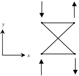
Elementary arguments based on the dimension of the transfer matrix of a repeating cell can lead to restrictions on the possible coupling of eigenvectors, and in turn the possible JCF. Consider the simple planar cell shown infigure 6: as there are two displacement degrees of freedom per node, so the stiffness matrix Kand the transfer matrix G are both of size ð8!8Þ. As with any straight planar structure, there must be precisely six unity eigenvalues—rigid body displacement in the x-direction and tension are coupled within a ð2!2Þ Jordan block, while rigid body displacement in the y-direction, cross-sectional rotation, bending moment and shear, are coupled within a ð4!4Þ Jordan block. Thus, the Jordan block structure must take the form

l 0 0 lK1

1 1

1

1 1

1 1

1 1

1 2

6 6 6 6 6 6 6 6 6 6 6 6 6 6 6 6 4

3 7 7 7 7 7 7 7 7 7 7 7 7 7 7 7 7 5

; ð7:2Þ

where the single unknown eigenvalueloccurs as a pair with its inverse, and with a possible unity element replacing the zero to its right. Now a necessary, but not sufficient, condition for a principal vector to be coupled to an eigenvector, when one does have a unity on the superdiagonal in that block, is that an eigenvalue is repeated; for a matrix of this dimension this can only occur whenl_ZlK1_{, which in} turn implies l_ZG1. The repeated eigenvalue l_ZK1, within a non-trivial block, does indeed occur for the cell, figure 4, which acts as a scissors-mechanism when subject to the self-equilibrated loading shown. A more general proof leading to the

x y

same conclusion that the only possible repeating eigenvalues which can give rise to a non-trivial Jordan block arel_ZG1 is now developed.

(a) Eigenvectors associated with l_ZG1 do no work If the left-hand side eigenvector is written as

e_Z dL pL

; ð7:3Þ

then the right-hand side vector is

leZ ldL

lpL " #

; ð7:4Þ

and the force and displacement vectors, according to the sign conventions of FEA, are

F_Z FL FR " #

Z KpL

lpL " #

; d_Z dL

ldL " #

: ð7:5Þ

Now the strain energy stored within the cell is equal to the work done (WD), which is

WD_Z1 2d

T F_Z1

2½d T L ld

T L

KpL lpL " #

Z1₂ðl2K1ÞdT_Lp_LZ1 2ð1Kl

2

ÞdTLFL: ð7:6Þ

Clearly, the WD is zero for lZG1. This agrees with experience: the only known eigenvectors havinglZ1 are rigid body translations and rotations, while the only

known eigenvectors having lZK1 pertain to structures having a partial scissors-mechanism, as infigure 4.

(b) Work associated with a principal vector

If the left-hand side principal vector is written as

p_Z d

p L

pp_L

" #

; ð7:7Þ

where the superscript ‘p’ denotes principal, then the right-hand side vector is

lpCeZ

ldp_LCd_L lpp_LCp_L

" #

; ð7:8Þ

and the force and displacement vectors are

FZ

Kpp_L lpp_LCp_L

" #

; dZ

dp_L ldp_LCd_L

" #

; ð7:9Þ

and the strain energy is

WDZ1₂dTFZ1₂½ðl2K1Þd pT L p

p LClðd

pT

L pLCdTLp p

rigid body displacement has no force components, and the second term reduces to WD_Z1

2d T Lp

p

L; ð7:11Þ

which is one-half of the extension (the displacement components of the eigenvector) times the tensile force (the force components of the principal vector). Now, it is known that principal vectors are not unique: one may add an arbitrary multiple, say b, of the generating eigenvector and it is still a principal vector, that is

GpZlpCe; ð7:12Þ

and also

GðpCbeÞZlðpCbeÞCe; sinceGbeZlbe: ð7:13Þ (On the other hand, one cannot arbitrarily add multiples of a principal vector of one grade to a principal vector of another grade.) Now re-calculate the work associated with the modified principal vector as follows: on the left-hand side one has

pCbe_Z

dp_LCbd_L

pp_LCbpL

" #

; ð7:14Þ

while the right-hand side state vector is

lðpCbeÞCe_Z

ldp_LCðlbC1Þd_L lpp_LCðlbC1ÞpL

" #

; ð7:15Þ

with cell force and displacement vectors

F_Z Kp

p LKbpL

lpp_LCðlbC1ÞpL

" #

; d_Z d

p LCbdL

ldp_LCðlbC1ÞdL

" #

: ð7:16Þ

The strain energy is then WD_Z1

2½ðl 2

K1ÞdpT_L pp_LCððl2K1ÞbClÞðdpT_L p_LCdT_Lp_LpÞCððl2K1Þb2

C2lbC1ÞdT_Lp_L: ð7:17Þ

Now make the assertion that the strain energy must be independent of arbitraryb, that is expressions (7.10) and (7.17) must be identical; this requires

Ab2CBbZ0; ð7:18Þ where

AZðl2K1ÞdTLpL; BZðl2K1Þðd pT

L pLCdTLp p

LÞC2ldTLpL: ð7:19Þ This assertion is equivalent to the demand that the strain energy should be independent of the choice of coordinate axes, since the eigenvectors are the rigid body displacements in thex- andy-directions. Now sinceb is arbitrary, equation (7.18) clearly requires that A_ZB_Z0. The former requires eitherðl2K1Þ_Z0, or dTLpLZ0, or both. Ifðl2K1Þ_Z0, then the requirementB_Z0 impliesdT_Lp_LZ0; if, from the requirement A_Z0, one chooses dTLpLZ0, with ðl2K1Þ_s0, the requirementBZ0 impliesdpTL pLCdT_Lp

p

LZ0. Thus, one has the two possibilities: (i) ðl2K1Þ_Z0 and dT_Lp_LZ0, or

Case (i) agrees with experience. However, the first scalar product of case (ii) implies the existence of an eigenvector associated with a non-unity decay eigenvalue, for which the strain energy in the cell and, indeed, the entire semi-infinite structure, is zero, which is inconceivable. Thus, one concludes that the only possible repeating eigenvalues that can give rise to a non-trivial Jordan block are lZG1. Karpovet al. (2002a)have recently classified possible modes in repetitive structures as ‘exponential’ (i.e. Saint-Venant decay according to a single non-unity eigenvalue), ‘polynomial’ (that is, transmission associated with multiple unity eigenvalues) and ‘quasi-polynomial’ (that is, degenerate multiple non-unity eigenvalues). It has been shown that these quasi-polynomial modes cannot exist.

The above arguments presume the eigenvalues and vectors to be real; should they be complex, then the transpose of the displacement vector is replaced by the Hermitian conjugate (complex conjugate transpose), and one concludes that

ll_Z1, where ‘’ denotes the conjugate, in which case the only possibilities are the complex unity eigenvalues. Again, this is in accord with experience in the eigenanalysis of pre-twisted (Stephen & Zhang 2006) and curved structures (Stephen & Ghosh 2005).

8. The effect of cell (a)symmetry

In this section, we note that eigenvalue degeneracy is intrinsic to translational symmetry, which is the same as the structure being repetitive. In particular, eigenanalysis of a tapered cell reveals splitting of two unity eigenvalues. On the other hand, for repetitive structures for which the cell has additional symmetries, additional constraints (relationships) may be derived for both the stiffness and transfer matrices; this is explored for a cell having left-to-right (reflective) symmetry. Symmetry is synonymous with constraint.

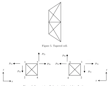
(a) Tapered cell

Consider the tapered, pin-jointed cell shown infigure 5, which is a modification of the cell shown infigure 2, in which the right-hand side vertical members have been increased in length to 1.5 m, and the diagonal members to suit. Clearly, such a cell cannot be part of a repetitive structure, since adjacent cells are obviously different; eigenanalysis is still a valid mathematical operation, but is not a practical proposition, as it would have to be repeated for each individual cell; nevertheless, some interesting observations arise. First, note that the eigenvalues still occur as reciprocal pairs

1 1 !

; 1

1 !

; 3=2

2=3 !

; 25:1235

0:0398 !

; 2:7890

0:3585 !

; K12:5159

K0:0799 !

;

ensure that the displacement components of the moment eigenvector should also transmit withl_Z2=3. Clearly, two of the unity eigenvalues must pertain to a rigid body displacement in the x-direction, coupled to a tensile force. The other two pertain to a rigid body displacement in the y-direction and a combined bending moment and shearing force vector. Shearing force and bending moment are no longer coupled within the same Jordan block.

(b) Cells having left-to-right symmetry

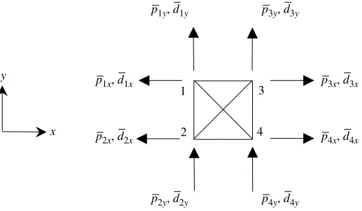
Consider the simple X-braced cell shown in figure 6, which clearly has left-to-right (denoted L5R) symmetry. In figure 6a, the nodal forces are shown according to the conventions of the Theory of Elasticity, and decay of a self-equilibrated loading applied to the left-hand nodes is assumed left-to-right, that is jlj!1. In reflecting the cell tofigure 6b, thex-components of force are in the same direction, while the y-components have changed direction. Similarly, the components of displacement in the x-direction will change sign, while those in the y-direction remain unchanged. The eigenvector for the left-to-right decay, written in full, is

sLZ½d1x d1y d2x d2y p1x p1y p2x p2y T

: ð8:1Þ

Now by virtue of the symmetry of the cell, the equivalentright-to-lefteigenvector, figure 6b, also having aright-to-leftdecay of jlj!1, will be

½Kd1x d1y Kd2x d2y p1x Kp1y p2x Kp2yTZRsL; ð8:2Þ Figure 5. Tapered cell.

p₁y

p₁x p₃x

p₃y

3 1

x y

2 4

p_1x

p₁y p₃x

p₃y

y

x

1

2 3

4

where the reflection (or parity) matrix Rmay be written in general as

R_Z A 0

0 KA

" #

; ð8:3Þ

and for the particular cell shown

A_Z

K1 0 0 0

0 1 0 0

0 0 K1 0

0 0 0 1

2 6 6 6 6 4

3 7 7 7 7

5: ð8:4Þ

For a planar structure, the essential pattern ofH1 on the leading diagonal will extend according to the number of nodes on the cross-section. For a three-dimensional beam-like space structure, the z-components of displacement and force would be unchanged by the L5R reflection, in which case the structure ofR

would be unchanged, while matrix A would consist of the sequence K1;1;1 repeated on the leading diagonal.

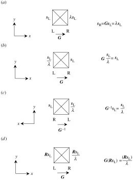
Since RsL is a right-to-left eigenvector having right-to-left decay with eigenvalue l, it is also a left-to-right eigenvector having left-to-right decay eigenvaluelK1_{. Thus, we may write initially,Gs}

LZlsL; pre-multiply byRGK1to give RGK1_s

LZlK1RsL. But from the symmetry argument above, one also has GRsLZlK1RsL. Symmetry demands that the two should be indistinguishable, which requiresGRZRGK1_{, orRGR}

ZGK1_{. Note that the reflection matrixRis} involutory, that is R2ZI, as is matrix A. These arguments are represented

graphically infigure 7. A more rigorous approach is presented in §8c.

(c) Four pole representation

Following Easwaran et al. (1993), who considered a four pole representation with positive state variables according tofigure 8, definebarredpositive force and displacement components according tofigure 9. This representation is ideal for the L5R symmetry of the cell; force components are related to the FE sign convention according to

p1x ZKF_1x; p_1yZF_1y; p_2xZKF_2x; p_2yZF_2y;

p3x ZF3x; p3yZF3y; p4xZF4x; p4yZF4y;

or

pL

pR " #

Z

A 0

0 I

" #

FL FR " #

; ð8:5Þ

while displacement components are related according to

d1x ZKd_1x; d_1yZd_1y; d_2xZKd_2x; d_2yZd_2y;

d3x Zd3x; d3yZd3y; d4xZd4x; d4yZd4y;

or

dL

dR " #

Z

A 0

0 I

" #

dL dR " #

Now define the stiffness matrix in this representation as

p_ZKd; ð8:7Þ

or more fully

pL

pR " #

Z

KLL KLR

KRL KRR

" #

dL

dR " #

; ð8:8Þ

which may be rearranged as

pR

pL " #

Z

KRR KRL

KLR KLL

" #

dR

dL " #

: ð8:9Þ

G

s_R=Gs_L=ls_L

R L

s_L

s_L

s_L

Rs_L

y

x

ls_L

G

R L

y

x

G–1 L R

y

x

G

R L

y

x

(a)

(b)

(c)

s_L G

s_L

l =

s_L

l

G–1_s L=

G(Rs_L) (RsL)

l

=

s_L

l

s_L

l

Rs_L

l

(d)

Now symmetry of the cell demands that equations (8.8) and (8.9) be indistinguishable, which requires

KLLZKRR; ð8:10aÞ

KLRZKRL: ð8:10bÞ

These barred stiffness matrix partitions can now be related to their conventional counterparts, as follows: first note

pLZKLLdLCK_LRd_R ð8:11aÞ and

FLZKLLdLCK_LRd_R: ð8:11bÞ Pre-multiply the latter by A, note that pLZAFL; dLZAdL; dRZdR, and subtract the former to give

ðAKLLKK_LLAÞd_LCðAK_LRKK_LRÞd_RZ0: ð8:12Þ Now since the displacement vectorsdL anddRare quite arbitrary, one must have

KLRZAKLR ð8:13aÞ

and

KLLAZAKLL ð8:13bÞ

or

KLLZAKLLA; ð8:13cÞ

since AK1

ZA: Similarly, one has

pRZKRLdLCK_RRd_R and F_RZK_RLd_LCK_RRd_R; ð8:14Þ

V_R

F_R V_L

F_L

input output

Figure 8. General four pole representation.

y

x

3 1

4 2

p_1y, d_1y

p_1x, d_1x

p_2x, d_2x

p_3x, d_3x

p_4x, d_4x p_3y, d_3y

p_2y, d_2y p_4y, d_4y

substitute pRZFR in the latter, and subtract the former, again noting that

dLZAdL, to give

ðKRLKKRLAÞdLCðKRRKKRRÞdRZ0; ð8:15Þ and hence

KRRZKRR and KRLZKRLA: ð8:16Þ Thus, the symmetry requirements, equations (8.10b) and (8.13a), yield

AKLRZKRLA or KLRZAKRLA ð8:17aÞ and

KRRZAKLLA or AKRRZKLLA: ð8:17bÞ In addition, the stiffness matrix is symmetric, in which case one knows that

KRLZKTLR; from equation (8.17a), this further implies thatAK T

RLZKRLAand KTLRAZAKLR. In themselves, these relationships have no explicit implications for partitions of the transfer matrix G.

The transfer matrix relationship may also be posed in terms of the barred state variables, as follows: from equations (8.5) and (8.6), note that

dL pL

Z

A 0

0 KA

" #

dL

pL " #

; ð8:18Þ

or more compactly

sLZRsL; ð8:19Þ

while

sRZsR: ð8:20Þ

Substitute into equation (2.1), where thenth andðnC1Þth sections are regarded as the left- and right-hand sides, respectively, to give

sRZGRsL: ð8:21Þ

Now, if the cell has left-to-right symmetry, then the subscripts ‘L’ and ‘R’ are interchangeable, that is

sLZGRsR: ð8:22Þ

Substitute (8.22) into (8.21) to give

sRZGRGRsR; ð8:23Þ

henceGRis involutory, that is

ðGRÞðGRÞZI ð8:24Þ

or

RGR_ZGK1_{; ð8:25Þ}

which is identical to the relationship derived by the previous, more heuristic, approach. A relationship can also be established for the JCF of such symmetric cells: substituting G_ZVJVK1 _{and its inverse G}K1

ZV JK1VK1 into equation

(8.25) gives

ðJBÞðJBÞ_ZI; ð8:26Þ

Expanding equation (8.24) into its square partitions leads to the relationships

GddAGddAKG_dpAG_pdA_ZI; ð8:27aÞ

GdpAGppAKGddAGdpAZ0; ð8:27bÞ

GpdAGddAKGppAGpdAZ0; ð8:27cÞ GppAGppAKG_pdAG_dpA_ZI: ð8:27dÞ

9. Conclusions

A variety of results pertaining to the elastostatic transfer matrix analysis of repetitive structures has been presented. Results previously known relate to the reciprocal eigenvalue properties as a consequence of the symplectic nature of the transfer matrix, bi- and symplectic orthogonality and the impossibility of complex unity eigenvalues for prismatic repetitive structures. Multiple unity eigenvalues are a particular feature of the elastostatic eigenanalysis, and the Moore–Penrose pseudo-inverse is introduced as a rational approach to the computation of principal vectors. It is shown that only the eigenvalues l_ZG1 can give rise to a non-trivial JCF, at least for the prismatic structure. An example of a structure for which the transfer matrix has repeating negative unity eigenvalue is one possessing a scissor-like mechanism. A planar structure, previously treated as pin-jointed, is reconsidered as rigid-jointed; the additional rotational nodal degrees of freedom give rise to new Saint-Venant decay modes—the number of transmission modes associated with unity eigenvalues is fixed—while the equivalent continuum properties are practically unaffected. This is in accord with the practice of treating real, rigid-jointed structures as pin-jointed, at least for small deflection elastic analysis. Symmetry implies restriction: a variety of relationships between partitions of both the stiffness and transfer matrices of a cell possessing left-to-right symmetry are derived; in contrast, one has splitting of unity eigenvalues for a tapered cell that lacks translational symmetry. The present elastostatic results may be seen as complementary to Langley’s (1996) analysis of wave motion energetics using transfer matrices.

References

Abraham, R. & Marsden, J. E. 1978Foundations of mechanics. London: Benjamin Cummings. Aoki, M. 1987State space modelling of time series. Berlin: Springer.

Brillouin, L. 1953Wave propagation in periodic structures. New York: Dover.

Dougall, J. 1913 An analytical theory of the equilibrium of an isotropic elastic rod of circular cross section.Trans. R. Soc. Edinb.49, 895–978.

Easwaran, V., Gupta, V. H. & Munjal, M. L. 1993 Relationship between the impedance matrix and the transfer matrix with specific reference to symmetrical, reciprocal and conservative systems.

J. Sound Vib.161, 515–525. (doi:10.1006/jsvi.1993.1089)

Gantmacher, F. R. 1959The theory of matrices, vol. 1. New York: Chelsea. Kailath, T. 1980Linear systems. Englewood Cliffs, NJ: Prentice-Hall.

Karpov, E. G., Stephen, N. G. & Dorofeev, D. L. 2002b On static analysis of finite repetitive structures by discrete Fourier transform.Int. J. Solids Struct.39, 4291–4310. ( doi:10.1016/S0020-7683(02)00259-7)

Langley, R. S. 1996 A transfer matrix analysis of the energetics of structural wave motion and harmonic vibration.Proc. R. Soc. A452, 1631–1648.

Mead, D. J. 1970 Free wave propagation in periodically-supported infinite beams.J. Sound Vib.13, 181–197.

Mead, D. J. 1996 Wave propagation in continuous periodic structures: research contributions from Southampton.J. Sound Vib.190, 495–520. (doi:10.1006/jsvi.1996.0076)

Meirowitz, L. & Engels, R. C. 1977 Response of periodic structures by the z-transform method.

AIAA J.15, 167–174.

Meyer, K. R. & Hall, G. R. 1991 Introduction to Hamiltonian dynamic systems and the N-body problem.Applied Mathematical Sciences, vol. 90. Berlin: Springer.

Ogata, K. 1990Modern control engineering, 2nd edn. Englewood Cliffs, NJ: Prentice-Hall. Pease, M. C. 1965Methods of matrix algebra. New York: Academic Press.

Stengel, R. F. 1986Stochastic optimal control. New York: Wiley.

Stephen, N. G. 2004 State space elastostatics of prismatic structures. Int. J. Mech. Sci. 46, 1327–1347. (doi:10.1016/j.ijmecsci.2004.07.008)

Stephen, N. G. & Ghosh, S. 2005 Eigenanalysis and continuum modelling of a curved repetitive beam-like structure.Int. J. Mech. Sci.47, 1854–1873. (doi:10.1016/j.ijmecsci.2005.07.001) Stephen, N. G. & Wang, P. J. 1996aOn Saint-Venant’s principle in pin-jointed frameworks.Int.

J. Solids Struct.33, 79–97. (doi:10.1016/0020-7683(95)00019-7)

Stephen, N. G. & Wang, P. J. 1996bSaint-Venant decay rates: a procedure for the prism of general cross-section.Comput. Struct.58, 1059–1066. (doi:10.1016/0045-7949(95)00237-5)

Stephen, N. G. & Zhang, Y. 2004 Eigenanalysis and continuum modelling of an asymmetric beam-like repetitive structure.Int. J. Mech. Sci.46, 1213–1231. (doi:10.1016/j.ijmecsci.2004.07.012) Stephen, N. G. & Zhang, Y. 2006 Eigenanalysis and continuum modeling of pre-twisted repetitive

beam-like structures.Int. J. Solids Struct.43, 3832–3855. (doi:10.1016/j.ijsolstr.2005.05.023) Synge, J. L. 1945 The problem of Saint-Venant for a cylinder with free sides.Q. Appl. Math. 2,

307–317.

Taussky, O. & Zassenhaus, H. 1959 On the similarity transformation between a matrix and its transpose.Pac. J. Math.9, 893–896.

Yong, Y. & Lin, Y. K. 1989a Propagation of decaying waves in periodic and piecewise periodic structures of finite length.J. Sound Vib.129, 98–118. (doi:10.1016/0022-460X(89)90538-5) Yong, Y. & Lin, Y. K. 1989b Dynamics of complex truss-type space structures. AIAA J. 28,

1250–1258.

Zhong, W. X. 1995A new systematic methodology for theory of elasticity. Dalian: Dalian University of Technology Press. [In Chinese.]

Zhong, W. X. & Williams, F. W. 1992 Wave problems for repetitive structures and symplectic mathematics.Proc. Inst. Mech. Engrs J. Mech. Eng. Sci.206, 371–379.

Zhong, W. X. & Williams, F. W. 1993 Physical interpretation of the symplectic orthogonality of a Hamiltonian or symplectic matrix. Comput. Struct. 49, 749–750. ( doi:10.1016/0045-7949(93)90077-Q)

Zhong, W. X. & Williams, F. W. 1995 On the direct solution of wave propagation for repetitive structures.J. Sound Vib.181, 485–501. (doi:10.1006/jsvi.1995.0153)

Zhong, W. X., Lin, J. H. & Qiu, C. H. 1992 Computational structural mechanics and optimal control—the simulation substructural chain theory to linear quadratic optimal control problems.