On steady and variable buoyancy forcing in the Atlantic, an idealised modelling study

(1)

ePrints Soton

research or study, without prior permission or charge. This thesis cannot be

reproduced or quoted extensively from without first obtaining permission in writing from the copyright holder/s. The content must not be changed in any way or sold commercially in any format or medium without the formal permission of the

copyright holders.

When referring to this work, full bibliographic details including the author, title, awarding institution and date of the thesis must be given e.g.

(2)

UNIVERSITY OF SOUTHAMPTON

FACULTY OF ENGINEERING, SCIENCE AND MATHEMATICS School of Ocean and Earth Science

On steady and variable buoyancy forcing in the Atlantic,

an idealised modelling study.

by

Marc A. Lucas

(3)

Graduate School of the

Southampton Oceanography Centre

This PhD dissertation by Marc A. Lucas

has been produced under the supervision of the following persons:

Supervisor:

Prof. Jochem Marotzke

Chair of Advisory Panel: Prof. Harry L. Bryden

(4)

Declaration of Authorship

I, Marc A. Lucas, declare that the thesis entitled ‘On steady and variable buoyancy forcing in the Atlantic, an idealised modelling’ and the work presented in it are my own. I confirm that:

• this work was done wholly or mainly while in candidature for a research degree at this University;

• where any part of this thesis has previously been submitted for a degree or any other qualification at this University or any other institution, this has been clearly stated;

• where I have consulted the published work of others, this is always clearly attributed;

• where I have quoted from the work of others, the source is always given. With the exception of such quotations, this thesis is entirely my own work;

• I have acknowledged all main sources of help;

• where the thesis is based on work done by myself jointly with others, I havemade clear exactly what was done by others and what I have contributed myself;

• Chapter 4 has been published as:

Lucas, M. A., J. J. Hirschi, J. D. Stark, and J. Marotzke, 2005: The response of an idealized ocean basin to variable buoyancy forcing. Journal of Physical Oceanography, in press.

(5)

ABSTRACT

FACULTY OF SCIENCE, SCHOOL OF OCEAN AND EARTH SCIENCE Doctor of Philosophy

ON STEADY AND VARIABLE BUOYANCY FORCING IN THE ATLANTIC, AN IDEALISED MODELLING STUDY

By Marc A. Lucas

(6)

Acknowledgements:

First of all, I would like to thanks Prof. Jochem Marotzke for giving me this opportunity to delve into the realm ocean modelling. His enthusiasm over these three years is gratefully acknowledged as is his insistence on addressing zero order problems. If I have learnt anything, then it must the importance of scientific rigour in all the aspects of research.

I would also like to thank Joel Hisrchi, without whom much of this work would not have happened. His passion for all aspects of oceanography is truly infectious and his constant probing and fascination for the various problems encountered, either theoretical or numerical are exemplary. The whole group benefited from his insights and I owe him much in terms of the analytical approaches used during my PhD. He was also a much appreciated and efficient “secondary supervisor” when Jochem left for MPI.

I would also like to thank John Stark for setting up the model and adding the various pieces of code to bring it up to date. He greatly reduces the amount of time I spent staring at an insipid piece of code in frustration.

Special thanks also to the member of my advisory panel, Prof. Harry Bryden and Prof. John Shepherd who insured that my research stayed on course and encouraged me to look at the bigger picture, beyond the realm of numerical modelling.

A special mention must go to Matt Palmer. Sharing an office with him meant that we could share our day to day frustrations and discuss various aspects of our work. I also learnt a lot about music, surfing and the Indian Ocean.

The physical oceanography group must also be mentioned, particularly Clotilde, Fiona and Johanna as well as Rachel, Hannah, Adam and Zoë. The weekly meetings allowed me to broaden my knowledge of oceanography in a friendly and relaxed environment.

Thanks also to all the fellow students at the SOC, particularly the Mediterranean crowd for providing and enjoyable social environment while I was in Southampton.

(7)

Table of Figures

Figure1-1: Schematic of the oceanic circulation, panel a) shallow, panel b)

intermediate and deep (Talley, 2003)...5

Figure1-2: Poleward heat transport in the ocean basins (Trenberth and Caron, 2001). ...6

Figure2-1: schematic of horizontal discretisation of the two types of grids. ...26

Figure2-2 :Density against temperature at level 5, S=35...30

Figure2- 3: Density against temperature at level 10, S=35...31

Figure2-4: meridional velocity contours at the equator on 3 grids. Colour contours are in cm/s. ...35

Figure2-5: Maximum overturning during Spin-up for Res1 and Res2...37

Figure2-6: Meridional overturning stream function (sv) for 2x2 and difference with 4x4 resolution...37

Figure2- 7: Zonally averaged temperature field (oC) in the upper 700 metres for 2x2 and difference with 4x4 resolution...38

Figure2-8: surface currents for the two resolutions. The units are cm/s...39

Figure3-1: Example of the restoring temperature profile (oC) for 3 temperature gradients, 28 in blue, 26 in red and 18 in green for set 1 and 1M(left panel) and set 2 and 2M (right panel). ...46

Figure3-2: Maximum overturning stream function against restoring temperature gradient for the 4 sets. ...47

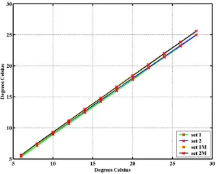
Figure3-3: SST gradient (y-axis) against restoring temperature gradient (x-axis) for the 4 sets. ...48

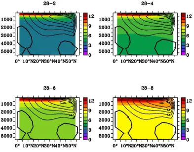
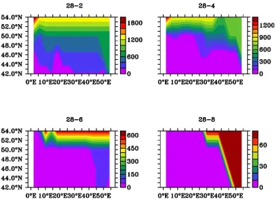
Figure3-4: Zonally average temperature field (colour shading) and meridional overturning stream function (black contours) for 4 experiments of set 1....49

Figure3-5: Depth integrated distribution of the convection index in the high latitudes (45o-60oN)...50

Figure3-6: meridional distribution of the zonally integrated convection index in the high latitudes (45o-60oN) from the surface to 1000 metres...51

Figure3- 7: zonal distribution of the meridionally integrated convection index in the high latitudes (45o-60oN) from the surface to 700 metres for set 2...53

Figure3- 8: meridional distribution of the zonally integrated convection index in the high latitudes (45o-60oN) from the surface to 700 metres...54

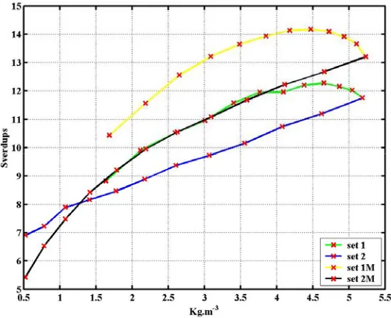
Figure3-9: Overturning against density gradient for the 4 sets...55

Figure3- 10: Meridional SST gradient between 45oand 60oN for 28-4 (black) and 24-0 (red)...56 Figure3-11: Depth integrated distribution of the convection index in the high

(11)

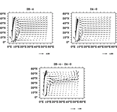
Figure3-12: Vector plot of the surface current for a temperature gradient of 28-4 (panel A) , 24-0 (panel B) and the difference between the two (panel C). ..58 Figure3-13: Bottom to surface average density difference at 60oN against

restoring temperature gradient for the 4 sets of experiments...59 Figure3-14: overturning against temperature gradient for set 1M and 2M...60 Figure3-15: a) Schematic of the effect of shallow depth convection on the

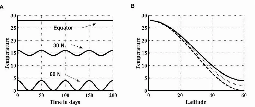
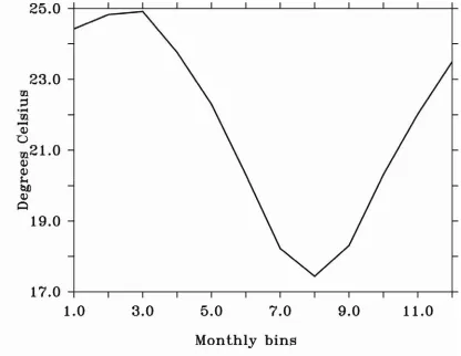
isopycnals at high latitude. The black curve is the initial shape of the isopycnal, the red curve is the modified portion of the isopycnal after convection has occurred in zone A, and the blue curve is the modified portion of the isopycnal after convection has occurred in zone B. b) zonal mean velocity, black initially, red after convection in zone A, blue after convection in zone B...62 Figure3-16: Temperature anomaly relative to the zonal mean at 800 metres for experiment 24-0 and 28-4 in the high latitudes...62 Figure3-17: generic zonal SST difference distribution...63 Figure 4- 1: Summary of variable forcing set-up. The left hand panel shows the evolution of the restoring temperature at 3 latitudes for a forcing period of 50 days. The right hand panel shows the maximum (solid line) and the minimum (dashed line) forcing profile as well as the forcing profile used to spin up the model (dotted line)...69 Figure 4-2: Monthly temperature gradient between the equator and 60oN in the Atlantic, obtained from NCEP data for the last 50 years...70 Figure 4-3: Panel A: Maximum overturning against time for experiment R1.

Vertical diffusivity is 1 cm2/s. The model is run for 17 forcing periods and for each until a cyclo-stationary state has been achieved.Panel B: Maximum overturning against time in experiment R1 for 4 successive forcing periods: 4, 8, 15, and 30 years. This Figure highlights the jump in amplitude in the overturning as the period increases from 8 years to 15 years. ...73 Figure 4- 4: Panel A: Maximum overturning against time for experiment R2. The diffusion is of 2 cm2/s. The model is run for 17 forcing periods and for each until a cyclo-stationary state has been achieved. ...74 Figure 4-5: Maximum overturning against time for experiment T1. The diffusion is of 1 cm2/s. The basin topography includes a north-south ridge 2500m high. The model is run for 17 forcing periods and for each until cyclo- stationary state has been achieved...75 Figure 4-6: Panel A: wind stress distribution for experiment D1 after Weaver & Sarachik (1990). ...76 Figure 4-7: Evolution of the minimum bottom temperature (solid) and the

(12)

Table of Figures

temperature is at a maximum, the north south temperature gradient is at a minimum. ...78 Figure 4-8: Evolution of the minimum bottom temperature (solid line) and the

forcing temperature (dashed line) during experiment R1 over the 1000 years forcing. This Figure shows the two components of the bottom temperature signal. ...79 Figure 4-9: Forcing temperature (dashed line) and overturning response (solid) in R1 for 9 forcing periods. The forcing temperature has been scaled up to the overturning and as a result, no absolute value can be inferred. The forcing temperature is the restoring temperature of the northern most (60o) latitude. Thus, when the forcing temperature is at a maximum, the north south temperature gradient is at a minimum...80 Figure 4-10: Evolution over one period of the convection (dotted line), the

Maximum overturning (dashed line) and the surface to bottom maximum temperature difference (solid line) for six forcing periods. All quantities have been normalised. The convection index is obtained by averaging over a sampling period the number of cells, which undergo convection...82 Figure 4-11: Evolution of the temperature (colour shading) and ψ (contours) over the four forcing periods: 8 (panel A), 250 (panel B), 2000 (panel C) and 32,000 years (panel D). The sampling period is set at 1/125 of the forcing period. The x-axis shows the normalised period...84 Figure 4-12: Maximum meridional overturning stream function for W1. The

vertical diffusion is of 1 cm2/s and the basin is 120o wide. The model is run for 17 forcing periods and for each until cyclo-stationary state has been achieved. ...87 Figure 4-13:Hovmoeller plots of the temperature anomaly at 800 metres depth at 30oN ,the normalised average surface temperature (red line) and the normalised restoring temperature (black line) for forcings periods of 8 years (panel A) and 60 years (panel B). The colour contours are in degrees Celsius and the Y-axis shows 2 normalised periods. ...88 Figure 4-14 :Panel A: maximum V velocity against time for Experiment R1:

The diffusion is of 1 cm2/s. The model is run for 17 forcing periods and for each until cyclo- equilibrium has been achieved. ...92 Figure5-1: Zonal extreme restoring temperature field for experiments 4-4, 4-4A, (in red and green) 4-5, 4-5A (in blue and black). During a forcing period, the restoring temperature field oscillates between the curves...99 Figure5-2: Spin up of asymptotic runs for a double hemisphere basin. ...100 Figure5-3: Example of the restoring temperature behaviour in the oscillatory

(13)

Figure5-4: Evolution of the PT and the overturning through a cycle for experiment 4-5. The contour intervals are of 2 Sverdrups...104 Figure5-5: Evolution of PT and overturning during a cycle in experiment 4-5A. The contour intervals are of 2 Sverdrups. ...105 Figure5-6: Overturning (colour shading) and zonally average Temperature

(black contour) at the equator over two periods, for experiment 5 and 4-5A for a forcing period of 2000 years. The y axis is depth in metres and the x-axis is time in fractions of a period...107 Figure5-7: Equatorial heat transport for 4-5A(red) and 4-5 (black) for a forcing period of 2000 years, over two periods. The y axis is in watts and the x-axis is time in fraction of a period. ...107 Figure5-8: maximum overturning stream function for experiment 4-5, in the

northern hemisphere (panel A) and the southern hemisphere (panel B)....109 Figure5-9: maximum overturning stream function for experiment 4-5A, in the

northern hemisphere (panel A) and the southern hemisphere (panel B)....110 Figure5-10: Hovmoeller plots for the northern hemisphere in experiment 4-5 for 4 forcing periods. The y axis is depth and the x-axis is time in fractions of a period. The contour spacing is of 5 Svredrups...112 Figure5-11: Hovmoeller plots for the southern hemisphere in experiment 4-5 for 4 forcing periods. The y axis is depth and the x-axis is time in fractions of a period. The contour spacing is of 5 Svredrups...113 Figure5-12: Hovmoeller plots for the northern hemisphere in experiment 4-5A

for 4 forcing periods. The y axis is depth and the x-axis is time in fractions of a period The contour spacing is of 5 Sverdrups...114 Figure5-13: Hovmoeller plots for the southern hemisphere in experiment 4-5A

(14)

Table of Figures

Figure5- 18: Temperature difference between level 1 and 15 (black curve, level 1 and 8 (red curve) and level 1 and 5 (green curve) in the Southern hemisphere. The y axis is temperature in degrees Celsius and the x-axis is time in fractions of a period. ...121 Figure5-19: Surface to bottom temperature difference for 4-4A(black), 4-5A

(15)

Chapter 1: Introduction

Summary:

In this chapter, the motivation behind this thesis is addressed. This is followed by a brief review of relevant topics namely, the North Atlantic and the Thermohaline circulation, the variability in data, the variability in models and fundamental modelling issues. Finally, a brief outline of the thesis is given.

1.1) Motivation:

The advent of numerical modelling has allowed the physical oceanographic community to take great steps in understanding problems that mathematical analysis cannot solve. Enormous progress in modelling has been made but some of the fundamental processes are still far from understood.

(16)

Chapter 1 Introduction

finite element adaptive grids models such as the one being developed at Imperial College, London (ICOM, 2004). However, these models are still in their infancy and most of today’s state-of-the-art ocean models are still based on the Bryan code written some 35 years ago.

This is not to say that there have not been significant improvements to the code. Particularly notable are the works of Redi (1982) of Gent and McWilliam (1990) in the domain of diffusion and eddy parameterisation. There has also been the development of isopycnal coordinates models such as MICOM (Miami Isopycnal Ocean Model), sigma coordinates models (Princeton Ocean Model) and Hybrid coordinates models such as Hybrid Coordinate Ocean Model (Bleck, 2002).

However, the lion’s share of improvements is the results of an increase in the resolution from coarse, 4ox4o non-eddy-permitting grids at the beginning of the last decade to the 1/12 o eddy-resolving grid of OCCAM (Ocean Circulation and Climate Advanced Modelling)(Webb, 1995). The increase in resolution is a direct result of the increase in processor speed and this increase was such that very quickly, physical oceanographers went from very basic ocean only process modelling with no or very simple topography to fully coupled ocean atmosphere scenarios with realistic topography. This was in part due to the growing awareness by the funding authorities of the uncertainties regarding a possible global warming and the need to have an idea of the possible scenarios (IPCC, 2001).

(17)

investigated. The aim of the present study is to address this particular gap in the modelling community’s understanding of the ocean circulation’s behaviour.

1.2) The North Atlantic and the THC:

The North Atlantic is the only region in the world where pure deep-water formation takes place. This is not a continuous process and occurs intermittently, during the coldest months of the year through deep convective events (Dickson & Brown, 1994). This does not mean that no deep water is formed anywhere else: there is deep-water formation in the Mediterranean for instance and of course in the Weddell Sea, where the world densest waters are formed. However, both the Mediterranean deep water and as the Weddell Sea Water are profoundly modified by cabelling and lose their distinct T-S signature very rapidly as they are carried away from the site of formation. By contrast the North Atlantic Deep Water (NADW) retains its T-S signature fairly well.

This deep water formation, which results from a combination of sinking and then cooling of the sinking waters is made possible by the high salinity of the Atlantic surface waters, which hovers around the 36 PSU mark, up to 3 PSU higher than North Pacific waters at similar latitudes (Pickard & Emery, 1990).

One of the reasons for this higher salinity is the moisture transport over the Isthmus of Panama. Crudely put, water evaporates in the Atlantic and is carried into the Pacific, where it precipitates, making the Pacific fresher and the Atlantic saltier. Another contributing factor to the high salinity levels in the Atlantic is the input of highly saline Mediterranean water as well as the contribution from the warm and saline Indian ocean through the shedding of Agulhas rings (Pickard & Emery, 1990).

(18)

Recent studies have shown that it is impossible to study the North Atlantic in term of freshwater budgets without considering the South Atlantic basin. Rahmstorf (1996) conducted a series of experiments which showed that the net evaporation in the subtropical South Atlantic and the southward fresh water transport by the conveyor belt are both compensated by a wind driven northward freshwater transport. This is in keeping with the conclusion of Schiller (1995). This means that freshwater budget north of 30oS is crucial to what happens in the north, i.e. how salty the North Atlantic will be. However, the freshwater water budget south of 30oS is function of the surface flow into the South Atlantic, via the Drake Passage and the Agulhas input through the shedding of the mesoscale rings.

Another factor affecting the salinity of the North Atlantic is the input of a fresh-water source through the Bering Strait. Its precise importance is not yet understood and there are diverging opinions regarding it. While Wijffells et al (1992) consider it highly important others like Reason & Power (1994) do not think it has any significant impact at all.

(19)

Figure1-1: Schematic of the oceanic circulation, panel a) shallow, panel b) intermediate and deep (Talley, 2003).

(20)

pumping and return to the regions of deep-water formation as surface waters, thus closing the circulation (figure 1.1).

Figure1-2: Poleward heat transport in the ocean basins (Trenberth and Caron, 2001).

(21)

It is widely reported is that the THC has several stable equilibria as has been shown in relatively simple ocean only model studies (Stommel, 1961, Rooth, 1982, Birchfield, 1989, Bryan, 1986, Kallen & Huang, 1987 Marotzke et al, 1988, Rahmstorf, 1995) and that a different THC configuration has existed in the past (Broecker, 1998). More complex coupled models have also exhibited these multiple equilibria (Manabe & Stouffer, 1988).

Today’s circulation is characterised by sinking in the high latitudes and is classified as thermally driven. This means that the flow is driven primarily by temperature differences. Theoretically, the sinking of water at low latitudes, driven by increasing salinity due to high evaporation is a perfectly sustainable alternative circulation set-up. Such a circulation is classified as haline driven but is thought to be highly unlikely (NRC 2002). It seems that the initial conditions determine which equilibrium will be achieved (Bryan, 1986). Moreover, some suggest that the present THC is very close to a bifurcation point. Increasing the freshwater input could well lead to a shutdown or a switch to an oscillatory regime (Rahmstorf, 1995).

The North Atlantic is thus a critical region in terms of the THC as it is one of the principal regions of deep-water formation. Any change to the properties of its surface waters will have a profound impact on the THC and hence on the global climate.

1.3) Variability in data:

1.3.1 )From decadal to Milankovitch climatic signals:

(22)

“abnormal” weather behaviour throughout the world even though oscillations, especially in temperature are common throughout the globe (Moron et al, 1998).

Another well studied interannual variability is the North Atlantic Oscillation, also called the northern hemisphere annular mode, which has been responsible for the succession of warm winters that Europe has experienced in the last 10 years. During its positive phase, the strength of mid-latitude zonal winds increase, trapping the cold Artic air in the northern Latitudes. As a result, winters in Europe are mild and wet (Thompson & Wallace, 2001). The NAO’s most common feature is a variation in sea level pressure around the Azores and Iceland but it can also be picked up in by variations in surface temperatures (Curry and McCartney, 2001). A detailed study of the interdecadal variations and the Atmospheric conditions that accompany them was conducted by Kushnir (1994). He found that there was not a lot of coherence between the SST anomalies behaviour and sea level pressure anomalies and associated wind anomalies. This hinted in his opinion to the fact that the interdecadal variabilities were controlled by a basin wide dynamical interaction between oceanic circulation and atmospheric processes.

(23)

indirect effect through the ENSO impact on tropical North Atlantic SST has been presented in some studies (Chiang et al, 2000, 2002)

Hydrographic studies over the last 30 years, particularly analysis of repeat sections of the ocean have also suggested a certain amount of fluctuation in the properties of the deep ocean, in the Atlantic (Lavin et al, 2003) and in the Indian Ocean (Bryden et al, 2003). Such studies have underlined variations in temperature, salinity and meridional transport (Lavin et al, 1998). However, the precise nature of these fluctuations, i.e. whether they are oscillations, red noise or trends is still uncertain.

All the variations discussed so far are of relatively high frequency. There are other oscillations of longer periods, which have been exposed by the study of Palaeodata, such as the Dansgaard/Oeschger and Heinrich Events, which oscillate on a millennial time scale. These events are known to influence the behaviour of the THC in the North Atlantic by varying the penetration of the sinking of surface waters and, as a result, the nature of the deep water (Alley et al, 1998). Succinctly, a Heinrich event corresponds to a period of massive ice rafting leading to a freshening of the surface waters. This means that the waters do not sink as deep. There is therefore an influx at depth of deep water from the Southern Hemisphere (Vidal et al, 1997). Dansgaard/Oeschger cycles refer to millennium scale climatic oscillations detected in ices cores from Greenland (Dansgaard et al, 1993). This translates to rapid warming or cooling of up to 16oC in the air temperature. Overlying these cycles is the longer period Bond Cycle, which has a period of roughly 6000 years (Alley, 1998) and corresponds to a warming/cooling of air temperature. The important point is that these events are thought to be independent of the glacial interglacial climate state, and are as such “pervasive millennial scale events” (Bond, 1997).

(24)

Precession refers to the angle of the earth’s axis to the stars; it has a period of 19,000 to 23,000 years depending on the eccentricity. The obliquity is the angle between the plane of the equator and the earth’s orbiting plane. Its period is roughly 41,000 years. Finally, the eccentricity refers to the elliptical shape of the earth orbits and its fluctuation between an almost perfect circle and a stretched out ellipse. The periods of the eccentricity are 54, 106 and 410 Ka (House, 1994).

There is evidence that these cycles affect climate in more ways than just by regulating the size of the ice sheets. Accurately forecasting their effect on the earth system is not an easy task and requires advanced climate models. A simple energy balance feedback model will not take into account all the various feedbacks, which influence the SST (North et al, 1981).

In a more recent attempt to fully model the orbital variations effect on the Sea Surface Temperature (SST), a numerical experiment by Sloan and Huber (2001) involving an Atmosphere coupled to a single layer shallow ocean showed that SST varied by as much as 6oC for two extreme points of the obliquity orbital cycle. They concluded that most of this variation was due to the presence of sea ice. Added to these SST variations was also a strong fluctuation in the wind fields at the surface of the sea.

(25)

1.3.2) Amplitude of the SST variabilities:

By analysing the δ18O isotope records from various sites in the North Atlantic for the last 1.1 MA, Ruddiman et al (1986) concluded that maximum SST variations at about 60o north were in excess of 10oC for summer and winter temperatures. This is also the estimate obtained by the Climex project in their world maps of the last two climatic extremes, namely 18,000years ago, the last glacial maximum and 8,000 years ago, the Holocene optimum (CGCM, 1999).

The same order of magnitude for variations can be found for temperatures over Antarctica in the last 400,000 years. Although these are land temperatures, they vary by up to 16oC (IPCC, 2002). This indicates that SST variations of about 6oC at 60o of latitude are plausible. Such an indicator is useful because of recent developments in palaeostudies, which imply that many previous findings might have been flawed (Pearson et al, 2001).

1.3.3) Palaeoceanography Methods:

There have been several approaches in Paleoceanography to determine SSTs in the past. In the late seventies, the chosen method was identification of foramanifera, a calcite shelled zooplankton found in a sediment core and comparing it with present day species. Working on the assumption that similar species live in similar habitats, i.e. similar temperature and depth, researchers were able to determine the SST bracket in which the forams found in the core lived. Thus, after dating the core, either through carbon dating or deposition rates, they could work out past SSTs. It was through this method that most of the Climap data was obtained. For 60o North, Climap gives a range of SST temperatures of about 8oC (IRI, 2002) between the two climatic maxima.

(26)

the two isotopes, the lighter isotope escapes more easily during evaporation, while the heavier isotope precipitates more easily. At low latitudes, net evaporation produces vapour which is depleted in 18O. As atmospheric circulation transports this vapour poleward, the on going precipitation en route causes the remaining water vapour to become progressively depleted in 18O. This process is also called Rayleigh Distillation (Libes,1992) The Rayleigh Distillation of water vapour also causes polar ice to be depleted in 18O relative to seawater.Thus, during an ice age, an increase in ice volume causes the ocean to be enriched in 18O. In addition to recording the oxygen isotope signature of ice volume, biogenic carbonates also reflect the water temperatures under which the foram shells were deposited.

The oxygen fractionation in a foram shell varies from specie to specie but can also be affected by the presence of symbionts, light levels and other factors (Bemis et al, 1998). But the comparison of data from various sites as well as laboratory experiments on modern species has enabled scientists to dissociate the various effects and work out reasonably accurate empirical equation giving the temperature of the waters in which the forams lived. Providing that the species examined are surface water dwelling and that their ages are known, past SST temperatures can be inferred (Savin et al, 1985).

(27)

The bottom line seems to be that care must be taken when looking at SST as derived from Oxygen isotope analysis. Furthermore, it is important to remember that the data obtained in cores is very localised and that care must be taken when extrapolating the results obtained for a few sites to a whole sea or portion of an ocean.

Finally, extra care must be taken when looking at very long SST records such as those available for Antarctica. It is possible to get SST estimates for the past 60 Ma. However, during this period, the world experienced significant tectonic alteration such as the closure of the Tethyan gateway and the opening of the Drake Passage. These changes were probably responsible for a drop of up to 18oC in SST, swamping any orbital and smaller period fluctuations (Open University, 1997). Furthermore, the oceanic circulation, prior to those changes was significantly different to today and therefore not really comparable. Indeed, some studies suggest that in the presence of a closed or shallow Drake Passage, there would be no production of NADW (Sijp and England, 2004) and as a result, the northern hemispheres temperatures would be colder.

A very useful parameter for determining past oceanic circulation is the deep-sea temperatures. Many oxygen based studies suggest that in the past, the deep waters were warmer than at present, by as much as 12o_{C 70 million years ago.}

(Zachos et al, 2001). The use of other proxies such as the Magnesium calcium ratio confirms this idea (Lear et al, 2000) and allows the dating of the major icing events in Antarctica.

(28)

feasible. It is even possible for the ocean to switch from one circulation pattern to another (Stocker, 1998). Such an event could have brought about the release an enormous amount of gas hydrates and thus caused the relatively sudden PETM (Palaeocene Eocene Thermal Maximum) warming 55 million years ago (Bice & Marotzke, 2002).

Recent methods now allow scientist to have a better handle on the past behaviour of the THC in the North Atlantic. McManus et al, (2004) suggest that the strength of the THC in the North Atlantic is highly correlated with temperature. Hence a cooling event is associated with a decrease in the overturning and conversely, a warming with a speeding up of the circulation.

It is clear that observational analysis, either by direct measurements or by the use of proxies reveals many variabilities in oceanic quantities such as temperature, salinity and forcing fields. The question is how well models can reproduce these and if they can provide a reasonable explanation for them.

1.4) Variabilities in Models

The study of variabilities in the ocean has largely involved numerical simulation, mostly because of a “lack of understanding of the physics of this type of variability” (te Raa & Dijkstra, 2002). Of all the variable time scales mentioned

earlier, the most studied appears to be the decadal to interdecadal scale. This is because to study longer time scales requires longer integration time not really feasible in the past.

(29)

Sarachik (1991) went on to show the advective origin of the oscillations but were unable to pinpoint the precise mechanism. Weaver et al (1993) showed that these oscillations were still present under varying evaporation-precipitation fluxes.

The three dimensional aspect of the oscillations was established by Winton (1996) as he found that they did not appear in 2D models. This is in disagreement with the results of Aeberhardt et al. (2000), who found oscillations in a zonally average ocean atmosphere coupled model. Winton (1996) also found that weak stratification at high latitudes, common in earlier models, impeded wave propagation and could thus lead to the decadal variabilities.

It was later suggested by Greatbatch and Peterson (1996) that the oscillations in the THC were generated by the propagation of a boundary trapped Kelvin wave and that therefore the western boundary was crucial to the existence of the oscillations.

The importance of the western boundary current seems to have been disproved by Huck et al (1999) who found that none of the boundaries was fundamental to the oscillatory behaviour. They also found that the wider the ocean basin, the greater the amplitudes and the periods of the oscillations. Their conclusion was that the dynamical link between the north-south pressure gradient and the overturning induced a time lag, which was fundamental to the oscillatory behaviour. Furthermore, in agreement with Winton (1997) and Weaver et al (1996) they found that realistic bottom topography damped out these oscillations: it is therefore unlikely that they would be found in the real ocean.

(30)

oscillations present in models are generated by the models themselves or by the phenomena modelled.

However, there are cases of studies where the oscillations found in the models roughly match those observed. For instance, Delworth and Mann, (2000), found in their runs oscillations of a seventy year period similar to those observed by Kushnir(1994). They noted however that the SST anomaly pattern was far closer to observations than the SLP (Sea Level Pressure) anomaly pattern, which exhibited a definite time lag compared to the patterns observed. Delworth and Mann (2000) concluded that these variabilities resulted from low frequency atmospheric noise interacting with feedbacks from the THC.

In the particular case of the North Atlantic, until recently there has been generally less awareness and interest of naturally occurring interdecadal variabilities among both the scientific and lay communities. This is mainly because the phase and amplitude of the oscillations observed were thought to be totally unpredictable (Hurrell et al, 2001).

This does not mean that no research was conducted. In the early 90’s, Delworth et al (1993) noted that a coupled GCM model of the North Atlantic exhibited interdecadal oscillation, albeit highly irregular, in the atmospheric signals similar to those observed in the real ocean. They concluded that these oscillations were driven by density anomalies in the vicinity of the sinking region.

(31)

decreased and for an interdecadal forcing period, there was either a basin wide increase or decrease. The authors also showed that under persistent forcing, the ocean could switch from a dipole to monopole SST pattern.

More recently, Delworth and Greatbatch (2000) revisited the NAO issue by using ocean only and coupled model runs. They concluded that a strong ocean-air interaction was not necessary to the generation of multidecadal variabilities. However, this does not mean that this is not the case in the real world.

The NAO does not only have an effect on SST and winds. It has also a distinct variability in the pressure distribution. Curry and McCartney (2001) looked at the effect of the varying pressure field and found that these considerably influence the gyre circulation in the North Atlantic.

Other studies have looked at the interdecadal oscillation problem from a numerical point of view. One such study was conducted by te Raa and Dijkstra (2002). They used a spherical coordinate implicit model to try to determine the physics behind the interdecadal oscillations. They pointed out that it was first necessary to distinguish between the growth of perturbations under unstable conditions from the physical mechanism that causes oscillatory behaviour, i.e. isolate what is specific to interdecadal oscillations.

(32)

Huck, (1999), if not a bit more elaborate. The latter pair concluded that the driving mechanism behind the oscillations were baroclinic instabilities, the term they give to the instability in the buoyancy work term.

There have also been efforts to study the oceanic response to Milankovitch orbital forcing. Brickman et al (1999) conducted a study using a 2.5D atmosphere ocean model run for 3.2 Ma. They found that the strongest response was in the obliquity band while the response in the eccentricity band was suppressed. Their explanation for this was that the main effect of obliquity was to control the seasonal contrast, and as deep water formation happens in winter, the harsher the winter, the greater amount of deep water formed and the stronger the overturning. Their results also showed that in the obliquity band, the global ocean average temperatures were negatively correlated with the atmospheric ones, due to a rectifying effect by the ocean. Their main conclusion was to highlight the complexity of the ocean system response and that, hence, care should be taken when interpreting deep-sea sediment cores.

1.5) Modelling Issues:

1.5.1) Mixing:

(33)

in the vicinity of rough topography in the Brazil basin. It is still unclear however, as to whether or not tidal energy and its dissipation is sufficient enough to close the MOC. Some studies suggest that the tilting of isopycnal in the southern ocean due to intense Ekman pumping may also play an important role in closing the MOC (Webb & Suginohara, 1997).

Within the numerical community, simultaneously to trying to understand various processes through the use of models, a lot of effort has been put into developing and improving numerical models. Most model used nowadays are derived from the original code written by Bryan (1969) and then further improved by Semtner and Cox (Kantha & Clayson, 2000).

In the last two decades, one of the most significant developments has been the improvement of the mixing scheme. The first step was to parameterise the fact that, in the ocean, a large part of tracer mixing consists of down gradient diffusion along isopycnals (Redi, 1982), which are not necessarily horizontal, especially at high latitudes (Danabasoglu and Mc William, 1995). In the original code, the mixing was handled by horizontal and vertical diffusion coefficients. As a result, the diapycnal mixing tended to be overestimated. Cox (1987) produced an isopycnal mixing parameterisation but the scheme contained a numerical instability, which meant that it could not be run without a non-negligible amount of background diffusion. As a result, the models tended to over diffuse and tracer properties were not well preserved over great distances, in contrast to observations (Griffies et al, 1998)

(34)

Griffies (1998) later found that GM mixing could also be handled through eddy skew diffusive fluxes. The advantage of this approach lies in the fact that it can be relatively easily combined with Redi (1982) diffusion and thus not only improve ocean modelling but also reduce the computational cost of the Redi (1982) diffusion scheme alone by a factor of 2.

The results are cooler deep waters, a shallower and sharper thermocline and a slight reduction in the overturning. Generally, model runs with isopycnal mixing yield results closer to observations than horizontal mixing runs. (Danabasoglu and McWilliam, 1995, Kamenkovich et al, 2000). These findings are very similar to those of Park and Bryan (2001) who compared three types of models: z layered with horizontal mixing, z layered with GM mixing and an isopycnal layered model. They looked at velocitiy fields, temperature profiles and the flow at the boundaries. They concluded that, although the three models had almost identical zonally averaged properties, the isopycnal model yielded the results, which were the closest to observations.

Danabasoglu and Mc William (1995) also found an increase in heat transport, in contrast to Kamenkovich et al (2000) who reported that the heat transport varies only very slightly, even though the overturning does decrease. Their explanation is that the decrease in overturning is compensated by the greater surface to bottom temperature gradient. They also suggest that the strength of the overturning results from the interaction of two competing effects. On one hand, reduced mixing in the high latitudes leads to a decrease in the mass overturning at low latitudes and hence a reduction in the overturning. On the other hand, reduced diapycnal mixing allows a greater amount of NADW to reach the low latitudes. They concluded that details in the model configuration such as topography, determine which of the two effects dominate, and whether the overturning will increase or decrease by comparison with a horizontal mixing setting.

(35)

the fact that, in the ocean, mixing is not uniform, far from it. It has been known for some time that a lot of the mixing takes place in shallow shelf seas, at the edges of ocean basins, driven by tidal and wind forces. As mentioned earlier, recent work suggests that a considerable amount of mixing also takes place in the deep ocean, as tidal and internal waves break on steep topography (Egbert & Ray, 2000). This suggest that some of today’s models basic parameterisations are fundamentally wrong and that the main control on the strength of the THC within an ocean basin is not the pole to pole surface density difference, a common concept amongst physical oceanographers (Rahmstorf, 1996) but rather the tidal and wind distributions (Wunsch, 2000).

This contrasts slightly with the findings of Marotzke and Scott (1999), who undertook the study of the convective mixing term. Using a 3D model, they investigated the oceanic circulation with 3 values of the convective mixing term: 0.1, 1 and 10 cm2/s. They found that the maximum overturning varied by only 1.5% for changes in the mixing term of 2 orders of magnitude. This led them to conclude that the strength of the overturning is primarily controlled by the strength of the diapycnal mixing but also by the surface density difference. They also found that increasing the convective mixing leads to a decrease in the overturning. In effect, mixing is important at low latitudes as it allows the deep waters to upwell but the rate of convective mixing, which occurs at high latitude has little impact on the strength of the overturning (NRC, 2002).

There have been some efforts in the numerical community to implement a more realistic mixing parameterisation scheme, such as the work by Simmons et al, (2004) where they use a global tidal model to compute the turbulent energy levels in the ocean and incorporate their parameterisation in a coarse resolution ocean model. The results are promising but such work is still in its infancy.

1.5.2) Sinking:

(36)

latitudes. For many years, the general assumption was that water was cooled by the atmosphere, its density increased, and as a result it sank (Gordon, 1986).

Winton (1996) used a 2D model to study the processes that led to very narrow sinking regions. He showed that a narrow sinking / broad upwelling system had two interesting energetic properties: upwelling occurred over a wide area to allow for the maximum penetration of heat through diffusion, thus the greatest overturning for a given forcing and a system with a narrow sinking region had the lowest potential energy possible because the deep is filled with the coldest possible waters, formed where the surface temperature is the coldest. As highlighted by Marotzke and Scott (1999), his approach is slightly flawed in that he used a 2D model, which is unable to resolve the 3D behaviour of the processes involved.

Clearly, in a 2D model, sinking and cooling are co-located. In a 3D environment, this has been shown not to be the case. Sinking and cooling are not necessarily co-located (Marotzke, 2000).

(37)

and convective mixing, can be co-located in regions of steep topography, i.e. in the Labrador sea.

1.6) Thesis layout:

As discussed above, the North Atlantic has some unique characteristics, which set it aside from the rest of the world’s oceans. Furthermore, the climate system has many variabilities ranging from the seasonal to the decadal to millennial timescales. This thesis examines the effect that simple buoyancy forcing has on the THC in the Atlantic, whether the forcing is steady or oscillatory. Specifically, the objectives of this study are:

• To examine the response of an idealized ocean basin to steady buoyancy forcing and provide an explanation for the observed breakdown of the scaling law.

• To examine and analyse the behaviour of the MOC in a single

hemisphere basin submitted to oscillatory buoyancy forcing.

• To examine and analyse the response of the MOC to oscillatory

buoyancy forcing in a double hemisphere basin.

In chapter 2, the models used are presented. The fundamental properties of the principal model, MOMA (Webb, 1996) are described in detail. A brief discussion of the effect of resolution is also given. Finally, the issue of visualisation is succinctly addressed in term of two fundamental quantities, the meridional overturning stream function and the heat transport.

(38)

temperature gradient to meridional overturning stream function is revisited and investigated in term of the distribution of convection. The experiments are carried out with two models, MOMA and the MIT model (Marshall et al, 1997) in order to determine whether or not the observed behaviour is model dependent.

In chapter 4, the response of the circulation to variable buoyancy forcing in a single hemisphere is investigated. Different diffusion and basin configurations are applied. In total 17 forcing period ranging from 6 month to 32,000 years are studied. The sensitivity of the response to basin width and diffusion is highlighted.

In chapter 5, the basin is increased to a double hemisphere. The response of the circulation to an oscillatory buoyancy forcing is investigated under two restoring scenarios: one where the forcing is synchronous in both hemispheres, the other with a lag of half a period. For each scenario, a range of north-south temperature gradient is examined.

(39)

Chapter 2: Model descriptions and visualisation

Summary:

This chapter presents a detailed overview of the MOMA model used in this study. A description of the initial fields is provided as well as an analysis of the important features of the model such as the equation of state. The method of visualising the model outputs is also examined, as is the effect of resolution. Finally, a brief description of the MIT model used in chapter 3 is given.

2.1) The MOMA model:

2.1.1) Introduction:

(40)

Chapter 2 Model descriptions and visualisation

The equations used, often called the primitive equations, are as described by Bryan (1969). As in most ocean models, in order to reduce the computational workload, three major approximations are used:

• In the continuity equation, the ocean is assumed incompressible.

• In the vertical momentum equation, the vertical acceleration is assumed negligible (hydrostatic approximation).

• The density is replaced by a constant value except in the terms involving the gravitational constant (Boussinesq approximation).

2.1.2) Ocean Grid:

The ocean is subdivided into small 3D boxes: in the Horizontal, the model uses a Arakawa B grid, where the horizontal velocities are defined at identical points offset from the tracers (see figure 2.1). This grid is well adapted to coarse resolution models although it does not represent well poorly resolved inertial gravity waves. It also offers a good representation of geostrophy as the velocity points are co-located (Griffies et al, 2000). One of itsdraw-back is that it slows down very fast waves such as Kelvin waves. It does however handle Rossby waves very satisfactorily (Wajsowicz, 1986, Dukowicz, 1995, Webb, 1996).

B GRID C GRID

Figure2-1: schematic of the horizontal discretisation of two types of grids. v

+

T,S

+

T,S u

(41)

The lateral boundary conditions in all the runs are no slip, non porous, which are naturally implemented in an Arakawa B grid. In the vertical, the ocean is divided into 15 levels. In order to have greater resolution near the surface, the level thickness increases with depth, varying from about 30 metres at the surface to more than 800 metres at the bottom (table 2-1). Topography is modelled by designating each box either as an ocean box or a Land box.

Level 1 30.0 metres

Level 2 46.15 metres

(42)

2.1.3) Free surface:

MOMA uses a free surface code, which allows for the propagation of barotropic gravity waves as well as the direct introduction of freshwater to the model. It also avoids all the issues relating to the rigid lid approximation such as solving elliptic problems with realistic surface forcings and topography (Griffies et al, 2000).

2.1.4) Initial salinity and temperature fields:

In the original MOMA code, the salinity is initially set at 34.9 throughout the ocean. The temperature field is slightly more complex in the original program code. At all grid points below 2000 metres of depth, the temperature is set at 2o centigrade. In the upper 2000 metres, an estimation is produced for each tracer grid point from a 7th order polynomial. The polynomial is the best-fit curve obtained from the Levitus surface temperature. At three reference latitudes, a depth profile is given. These are used to anchor the polynomial at every depth.

2.1.5) Surface boundary conditions:

MOMA allows the user to choose between restoring boundary conditions for both tracers and mixed boundary conditions. In all the experiments in this study, mixed boundary conditions are used. This means that the salinity is forced through fluxes while the temperature is restored through a Newtonian dampening scheme. In all the experiments in this study, the restoring time scale usedin is 40 days and the salinity fluxes set to zero. In the original model code, the restoring surface temperature field is interpolated in the same way as the salinity from the Levitus database. However, in all the experiments in this study, an oscillating restoring field is used. The details can be found in chapters 4 and 5.

(43)

stress to zero. In chapter 4, a zonal wind stress is used in one of the experiments. It is identical to that of Weaver & Sarachik (1990).

2.1.6) Time-step:

The model is integrated forward in time by leapfrogging (Webb, 1996). However, this leads to instabilities for the diffusive terms so an Euler forward time step scheme is used for those. Furthermore, to avoid the splitting of the solutions, every 20 time step, an Euler backward time step is used. The main advantage of an Euler backward method is that it prevents the model from becoming unstable due to the diffusive terms in the equations (Griffies et al, 2000).

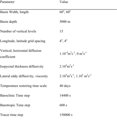
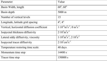
Parameter Value

Basin Width, length 60o, 60o

Basin depth 5000 m

Number of vertical levels 15

Longitude, latitude grid spacing 4o, 4o

Vertical, horizontal diffusion

coefficient 1.10

-4_m2_s-1_{, 0 m}2_s-1

Isopycnal thickness diffusivity 2.103_m2_s-1

Lateral eddy diffusivity, viscosity 2.103_m2_s-1_{, 1.10}5_m2_s-1

Temperature restoring time scale 40 days

Baroclinic Time step 14400 s

Barotropic Time step 600 s

[image:43.595.113.510.324.733.2]

Tracer time step 150000 s

(44)

To make the best possible use of the computational resources available, the time step should be as large as possible. The limiting condition placed upon the time step is that any disturbance must be contained within a cell during a time step. Consequently, the greater the resolution, the smaller the cell dimensions and the smaller the time step will have to be. In MOMA, the tracers and the barotropic and baroclinic velocities have independent time steps. This allows the model to be far more efficient as the tracer can handle much greater time steps without becoming unstable. This greatly reduces the amount of computations needed, since it integrates forward in time with the tracer time step, and then determines the variation of the horizontal velocities by using a single velocity time step. In such a configuration however, the model is only suited for the study of steady equilibrium solutions and not of transient behaviour (Griffies et al, 2000).

2.1.7) Equation of state:

(45)

Figure2-3: Density against temperature at level 10, S=35

(46)

2.1.8) Gent-Mc William Mixing

All the runs in this study include Gent McWilliams mixing (Gent & McWilliams, 1990) implemented through the Griffies (1998) parameterisation.

The aim of GM mixing is to parameterise the mixing effect of highly energetic eddies in the ocean. This is combined with the work of Redi (1982) which implemented the observation that most of the mixing occurs along density surface and not through them. The scheme involves introducing isopycnal tracer diffusivity (2.103m2s-1) and correcting the vertical and horizontal effect of diffusion accordingly. There is also a cut off angle for the slope of the isopycnal above which the GM scheme is not applied. This is to avoid spurious vertical mixing when the isopycnals are very steep such as in the high latitudes. Using GM mixing usually results in cooler bottom temperature as less heat from the surface diffuses down and a sharper thermocline as a consequence of the reduced diapycnal mixing (Kamenkovich et al, 2000). Furthermore, a slightly weaker overturning is found as a result of the weaker east-west density gradients due to the relative increase in the horizontal fraction of the mixing (Griffies et al, 2000).

2.1.9) Convection scheme

(47)

2.2)Visualisation:

2.2.1) Meridional overturning:

There are many ways of visualising the circulation in the ocean. However, in the case of a THC circulation, visualising the sinking and upwelling regions is of particular interest.

In order to so while simultaneously looking at the meridional behaviour of the circulation, one option is to calculate a proxy, called the meridional overturning. This scalar is defined from a triple integration of the continuity equation:

0 =

∂

+

∂

+

∂

z

w

y

v

x

u

where u, v, w are the zonal, meridional and vertical velocities respectively. The first integration is along the x-axis, i.e. from east to west of the u and v terms. This leads to the following expression:

x

y

v

x

z

w

E W E W

∂

=

∂

−

∫

where W is the western boundary of the ocean basin and E is the eastern one.

The following two integrations are along the vertical and the meridional length leading to the final expression of the meridional overturning:

z x y y v z x y z w z y E W Y z Z E W Y ∂ ∂ ∂ ∂ ∂ = ∂ ∂ ∂ ∂ ∂ − =

Φ

∫ ∫ ∫

∫

∫ ∫

− − 0 0 0 0 ) , (

∫ ∫

−

∂

−

=

Φ

(

,

)

0

z E

W

v

x

z

y

(48)

By definition, the meridional overturning is equal to zero at the bottom. In the case a free surface model, i.e where the surface is allowed to move up and down, it is easier to integrate the meridional overturning from the bottom upwards, especially when the bottom of the ocean is featureless, without any topography. Furthermore, in the case where there is no net mean transport, the meridional overturning is also equal to zero at the other vertical boundary.

2.2.2) Heat Transport:

Another important quantity to visualise is heat transport, particularly in the case of a double hemisphere basin as trans-equatorial heat transport in the ocean has a substantial impact on the global climate and deep-water formation. Bryan (1962) defines the total energy transport (Fq) in the ocean as follows:

∫ ∫

−

=

L

H p

q

c

v

dzdx

F

0 0

θ

ρ

where ρ is the density, cp the heat capacity at constant pressure, θ the potential temperature, H and L the depth and width of the section respectively. In models, this can be approximated by the following expression used for example by Stammer et al (2003):

∫ ∫

−

=

L

H p

q

c

v

dzdx

F

0 0

θ

ρ

(49)

Figure2-4: Meridional velocity contours at the equator on 3 grids. Colour contours are in cm/s.

There is however an issue with the model grid. The MOMA model uses an Arakawa B grid and as a result the meridional velocity and the potential temperature are not co- located. For the calculation to be as exact as possible, both quantities should be on the same grid. There are then three options: recalculate the value of v, the meridional velocity onto the potential temperature (θ) grid, recalculate the values of θ on the v grid or to recalculate both quantities onto an intermediate grid. Although this might appear trivial at first glance, in a model with coarse resolution, the differences can be quite substantial.

(50)

higher latitudes but this example underlines the care needed when computing quantities such as heat transport.

As the potential temperature field varies very little about the equator, the choice was made to recalculate PT and V on an intermediate grid, the x axis of which is that of PT and the y axis of which is that of V and then compute the heat transport. This strategy was deemed to yield the most sensible answer.

2.3) Comparison between 2

o

and 4

o

lateral resolution:

Lateral resolution can have a profound affect on the behaviour of an ocean model. In this study, a resolution of 4ox 4o is chosen mainly because of the integration time required to run the experiments. Indeed, halving the resolution not only reduces by a factor of four the number of cells, it also allows the timestep to be double. As a result, the total time gain obtained by halving the resolution is of a factor of 8.

Two identical runs but with two different resolutions are conducted to ascertain how substantial the difference are between a resolution of 4o_{x 4}o _{and a resolution} of 2ox 2o. Run Res1 has a resolution of 4ox 4o and run Res2 has a resolution of 2ox 2o. Both runs have a fixed restoring temperature profile which decreases sinusoidally with latitude from 28 degrees at the equator to 2 degrees at 60 degrees north. The vertical mixing is of 10 m-4/s in both cases and both runs have the free surface enabled as well as the Gent-McWilliams mixing.

(51)

Figure2-5: Maximum overturning during Spin-up for Res1 and Res2

(52)

12.04 Sv for the resolution of 4 degrees. This amount to a difference of 1.6 %, which is very small.

Figure 2-6 and figure 2-7 show respectively the structure of the meridional overturning and the structure of the potential temperature in the upper 700 metres at the end of the two runs. It is clears that there are some differences between the two runs. Figure 2.6 shows that the major differences in the overturning happen at low latitudes. This occurs because the overturning core extends further south for the resolution of 4ox4o resolution than for the 2ox2o resolution (not shown). The actual shape and maximum intensity of the overturning cell are almost identical in both runs. Furthermore, in both cases, the maximum overturning is located at 45oN and 1000 metres depth. Figure 2-7 shows that the isotherms behave similarly in both runs. As for the overturning, the greater differences occur at low latitudes, hence the difference in the amount of deep water formed at high latitude is very small (less than 1.5%).

(53)

Figure2-8: Surface currents for the two resolutions. The units are cm/s.

In figure 2-8, the surface currents are displayed. The western boundary current transport has approximately the same maximum value for both resolution, although it slightly greater for the 2x2 resolution. This occurs because in the 4x4 resolution, the WBC is only 1 cell wide whereas in the 2x2 resolution, it is 2 cells wide. This allows for a narrower WBC and thus, in order to get a similar mass transport, a greater velocity (in Res2, vmax= 16.44 cm/s, in Res4, vmax=13.10cm/s). It is interesting to note that the greater velocity occurs for the run with the smaller overturning. Outside the western boundary, the currents are almost identical for both resolutions.

2.4) The MIT model:

(54)

The MIT model is used in an identical setting as the MOMA model, with the same resolution, same forcing configuration (no wind, no salt fluxes, free surface and GM mixing implemented). It is however a far more modern model and many of its numerics are different from that of the older model. At a more fundamental level, it differs through the use of a horizontal C grid instead of a B grid for MOMA (figure 2-1). It also uses a third order Adams-Bashforth scheme instead of leapfrogging and synchronous time step for the velocity and tracers. These differences have repercussions in the representation of wave processes.

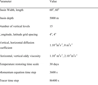
Parameter Value

Basin Width, length 60o, 60o

Basin depth 5000 m

Number of vertical levels 15

Longitude, latitude grid spacing 4o, 4o

Vertical, horizontal diffusion

coefficient 1.10

-4_m2_s-1_{, 0 m}2_s-1

Horizontal, vertical eddy viscosity 1.105 m2s-1, 2.10-3m2s-1

Temperature restoring time scale 30 days

Momentum equation time step 3600 s

[image:54.595.116.509.292.632.2]

Tracer time step 86400 s

Table 2-3: Summary of numerical parameters and diffusivities in the MIT model.

(55)

is different from the MOMA approach which uses convective adjustment to deal with unstable stratification.

(56)

Chapter 3 On the scaling law in OGCMs

Chapter 3: On the scaling law in OGCMs

Summary:

(57)

3.1) Introduction:

The complexity of the primitive equations that govern the oceanic thermohaline circulation has driven efforts to find a simple relationship that allows some form of prediction of the strength of the overturning given some simple climate parameters such as the equator to pole temperature difference. Very early on, Bryan and Cox (1967) suggested that the vertical “advection-diffusion” balance (3.1) and the thermal wind balance (3.3) could be combined with the continuity equation (3.2) to produce a scaling relationship giving the dependence of V, the horizontal velocity to ∆T, the equator to pole temperature difference and κ, the vertical diffusivity: L T f g D V D W L V D W ∆ α κ ~ ~ ~ (3.1) (3.2) (3.3)

where W is the vertical velocity, L is the horizontal length scale, D is the vertical length scale, g is the gravitational acceleration and f is the Coriolis parameter. Now, D L T f g V D L V ∆ ⇒ ⇒ α κ ~ ) 3 ( ~ ) 2 ( & ) 1

( ₂ (3.4)

(3.5)

which lead to the following expressions:

On steady and variable buoyancy forcing in the Atlantic, an idealised modelling study

ePrints Soton

On steady and variable buoyancy forcing in the Atlantic,

an idealised modelling study.

Graduate School of the

Southampton Oceanography Centre

Declaration of Authorship

Acknowledgements:

Table of Contents

Table of Figures

Chapter 1: Introduction

1.1) Motivation:

1.2) The North Atlantic and the THC:

1.3) Variability in data:

1.4) Variabilities in Models

1.5) Modelling Issues:

1.6) Thesis layout:

Chapter 2: Model descriptions and visualisation

2.1) The MOMA model:

+

+

2.2)Visualisation:

0

=

∂

∂

+

∂

∂

+

∂

∂

z

w

y

v

x

u

x

y

v

x

z

w

∂

∂

∂

=

∂

∂

∂

−

∫

∫

∫ ∫ ∫

∫

∫ ∫

∫ ∫

∂

∂

−

=

Φ

(

,

)

v

x

z

z

y

∫ ∫

=

c

v

dzdx

F

θ

ρ

∫ ∫