Ancient plant DNA in lake sediments by Parducci et al. 1
2
New Phytologist (2017) 214: 924–942 3
doi: 10.1111/nph.14470 4
5
Author final copy 6
7
This document is provided solely in order to be compliant with HEFCE requirements for REF. As 8
it may contain errors subsequently corrected in proof, NOTHING in it should be trusted. 9
10
Please use the final version on the publisher's website, or contact the authors for a final 11
published PDF that can be considered reliable. 12
Ancient plant DNA in lake sediments 14
15
Laura Parducci1, Keith D. Bennett2,3, Gentile Francesco Ficetola4,5, Inger Greve Alsos6, 16
Yoshihisa Suyama7, Jamie R. Wood8, Mikkel Winther Pedersen9 17
18
1Department of Ecology and Genetics, Evolutionary Biology Centre, Uppsala University, 19
Norbyvägen 18D, 75236 Uppsala, Sweden; 2Department of Geography & Sustainable 20
Development, School of Geography & Geosciences, University of St Andrews, KY16 9AL, 21
Scotland; 3Queen’s University Belfast, Marine Laboratory, Portaferry, BT22 1LS, Northern 22
Ireland, UK; 4Université Grenoble-Alpes, CNRS, Laboratoire d’Ecologie Alpine (LECA), F-38000 23
Grenoble, France; 5Department of Biosciences, Università degli Studi di Milano, 20133 Milano 24
Italy. 6Tromsø Museum, UiT – The Arctic University of Norway, NO-9037 Tromsø, Norway; 25
7Field Science Center, Graduate School of Agricultural Science, Tohoku University, 232-3 26
Yomogida, Naruko-onsen, Osaki, Miyagi 989-6711 Japan; 8Long-term Ecology Lab, Landcare 27
Research, PO Box 69040, Lincoln, Canterbury 7640, New Zealand; 9Centre for GeoGenetics, 28
Natural History Museum of Denmark, University of Copenhagen, 1350 Copenhagen, 29
Denmark. 30
31
Authors for correspondence: 32
Laura Parducci, +46 18 471 64 14, laura.parducci@ebc.uu.se; @lauparducci 33
Mikkel Winther Pedersen, +45 29 27 53 42, mwpedersen@snm.ku.dk; @miwipe81 34
35
Total word count for the main body of the text: 8995 36
Number of figures: 7 (all should be published in colour) 37
Number of tables: 1 38
Supporting information: Note S1 39
Summary 41
Recent advances in sequencing technologies now permit analyses of plant DNA from fossil 42
samples (ancient plant DNA, plant aDNA), and thus enable molecular reconstruction of 43
palaeofloras. Hitherto, ancient frozen soils have proved excellent in preserving DNA 44
molecules, and have thus been the most commonly used source of plant aDNA. However, 45
DNA from soil mainly represents taxa growing few meters from the sampling point. Lakes 46
have larger catchment areas and recent studies suggest that plant aDNA from lake sediments 47
is a more powerful tool for palaeofloristic reconstruction. Furthermore, lakes can be found 48
globally in nearly all environments and are therefore not limited to perennially frozen areas. 49
Here we review the latest approaches and methods for studying plant aDNA from lake 50
sediments and discuss the progress made up to present. We argue that aDNA analyses add 51
new and additional perspectives for studying ancient plant populations and in time will 52
provide higher taxonomic resolution and more precise estimation of abundance. Despite this, 53
key questions and challenges remain for such plant aDNA studies. Finally, we provide 54
guidelines on technical issues, including lake selection and we suggest directions for future 55
research on plant aDNA studies in lake sediments. 56
57
Keywords: ancient plant DNA, bioinformatics, environmental DNA, high-throughput DNA 58
sequencing, lake sediments, metabarcoding, shotgun sequencing, pollen, taphonomy 59
Introduction 61
62
Ancient DNA (aDNA) analysis is a young, but rapidly developing research field. Since the 63
pioneering work in the 1980s (Higuchi et al., 1984; Pääbo, 1984) there has been an 64
exponential increase in aDNA studies investigating evolution and ecology of the last 800 65
thousand years before present (kyr BP). 66
A Web of Science search on aDNA studies (January 1984-August 2016, keyword ‘ancient 67
DNA’), detected 2104 papers. Most focus on vertebrates, especially humans (50%), while only 68
5% focus on plants and ecology (Fig. 1). Ancient DNA from skeletal remains has been so much 69
easier to study than plant macrofossils, and the difficulty in getting aDNA from charred 70
specimens that represent 95% of the plant archaeological record, may partially explain the 71
lack of plant aDNA papers. Plant aDNA studies have been also delayed by the difficulty in 72
finding standard barcode regions useful for all species (universal) and sufficiently variable to 73
discriminate among taxa. Three important trends are evident from Fig. 1: (i) the total number 74
of studies has increased steadily through the last three decades; (ii) the number of opinion 75
and methodological papers accounts for most of the increase since ca 2004; (iii) after three 76
decades of aDNA research, plants continue to receive limited attention in relation to their 77
importance in the landscape. 78
Despite this, plant aDNA research has made dramatic progress with: (i) the recent adoption of 79
high-throughput DNA sequencing (HTS) technology; (ii) the discovery that DNA can be 80
isolated from fossil pollen (Suyama et al., 1996; Parducci et al., 2005); and (iii) the finding that 81
plant aDNA can be extracted from ice-cores, permafrost soil, lake sediments, coprolites and 82
peat cores (see Rawlence et al., 2014). Since the first research (Willerslev et al., 2003), a 83
number of studies on past biodiversity have been published using aDNA from a variety of 84
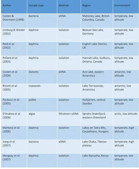
palaeoenvironments (ref. 3-18 in Pedersen et al. 2015). These studies (see also Table 1) show 85
how DNA can often identify more species and at higher taxonomical resolution than those 86
identified by pollen and macrofossil analyses, thus providing important ecological and climatic 87
information on the investigated sites otherwise difficult or impossible to infer (e.g. minimum 88
July temperature or nutrient conditions for taxa identified at species levels; Sønstebø et al. 89
2010, Parducci et al. 2015). DNA studies generally identify more herbs (Willerslev et al. 2014, 90
Alsos et al. 2016) and have greater taxonomic resolution for grasses, thus providing better 91
information on local biodiversity and for reconstruction of palaeoenvironments. The latter is 92
an advantage compared to pollen especially at high latitudes/altitudes where local pollen 93
The DNA field however, is not without technical challenges, for which specialised techniques 95
and protocols have been developed (Hofreiter et al., 2001; Chan et al., 2005; Shapiro & 96
Hofreiter, 2012). It is therefore timely to review recent progress on plant aDNA studies and 97
to suggest new directions for the future. We focus our review on lake sediments, because 98
their geological context provides a robust archive for retrieval of plant aDNA through time, 99
and because lakes can be found in all environments around the world. We synthesize and 100
discuss recent key findings on DNA from ancient pollen and sediment samples (see Table 1 101
form a complete list of studies) and in particular the progress achieved using HTS 102
technologies. Finally we discuss issues relating to false positives and the need for 103
authentication (i.e. replication, use of controls), taphonomic processes, and bioinformatic 104
challenges relating to the newest taxonomic identification and authentication of aDNA 105
sequences. 106
107
108
Environmental and temporal limits for survival of aDNA 109
The temporal limit of DNA preservation is dictated by the rate of degradation, which varies 110
depending on the source material and micro-environmental conditions. The most favourable 111
conditions (anoxic and frozen/cold) occur in permafrost and ice; here DNA can persist in 112
biotic remains and environmental samples (e.g. soils) for hundreds of thousands of years 113
(Lindhal, 1993; Hofreiter et al., 2001; Allentoft et al., 2012; Dabney et al., 2013; Orlando et al., 114
2014). Currently, the oldest authenticated plant aDNA sequences are from frozen 115
environments dated between 450 and 800 kyr (Willerslev et al., 2007). Such favourable 116
conditions however, are restricted to polar regions and high alpine environments. Plant aDNA 117
has also been successfully extracted and analysed from arid and hot environments (Hofreiter 118
et al., 2003; da Fonseca et al. 2015; Mascher et al. 2016), temperate middens and coprolites 119
(see Rawlence et al., 2014), suggesting that warm temperatures are not necessarily a barrier 120
for preservation of DNA molecules. 121
Several studies have investigated the post mortem processes affecting DNA molecules in 122
different tissues. We know that after the death of an organism, several intra and extra-123
cellular processes (e.g. enzymatic, hydrolytic and oxidative processes) cause DNA damage 124
(seen as misincorporation of C to T and G to A transitions primarily toward the ends of the 125
DNA molecules) (Briggs et al., 2007; Jónsson et al., 2013), eventually leading to fragmentation 126
frozen, anoxic or arid areas, environments with limited bacterial abundance and therefore 128
presence of nucleases, which reduces longer nucleic acids to short molecules (Hofreiter et al., 129
2001). Nevertheless, exogenous processes will inevitably lead eventually to the 130
destabilization, fragmentation and damage of DNA, even in good preservation conditions. 131
To determine the rate of DNA decay, Allentoft et al. (2012) quantified the temporal survival of 132
DNA molecules in bones. They found a half-life of 521 years for short [242 base pairs (bp)] 133
mitochondrial DNA (mtDNA) fragments preserved at ca. 13 °C. The fragmentation rate 134
however was strongly reduced at lower temperatures, and it was assumed that under very 135
cold and dry conditions short fragments should be retrievable from bone more than 1 million 136
years old. No similar studies exist for ancient plant tissues, and there are currently no 137
indications of an age limit for plant aDNA. Nevertheless, damage for plant DNA also 138
accumulates with age (Pedersen et al., 2016). So far, plant DNA has been recovered and 139
analysed from sediments >55 ka BP (Willerslev et al., 2014), from ice cores dated between 140
450 and 800 kya BP (Willerslev et al., 2007) and from pollen ca. ~150 ka BP (Suyama et al., 141
1996), which suggests that DNA studies from lake sediments can potentially span the Late 142
Pleistocene and Holocene. 143
144
145
Lake sediments 146
During the last decade, molecular ecologists have increasingly begun investigating Late 147
Quaternary floristic history using DNA isolated from pollen and DNA extracted from lake 148
sediments (pollen DNA and sedaDNA, respectively) for a number of reasons. We review these 149
below. 150
151
Lake sediment characteristics 152
Lakes are excellent sources of sediments containing aquatic and terrestrial environmental 153
components accumulated over time and preserved in robust stratigraphic contexts and 154
anoxic conditions. They offer the best settings for preservation of plant aDNA, as the 155
sediments accumulate continuously; allowing establishment of high-resolution molecular 156
records using available geo-chronological methods (Fig. 2a, b, c) and thus providing a robust 157
record for interpretation of the molecular history. In particular, sediment records from small 158
low and seem to represent the surrounding terrestrial environment well. Lake sediments 160
consist of variable proportions of autochthonous/allochthonous organic material (OM) and in-161
washed inorganic material. Microbial degradation of OM frequently creates anoxic conditions 162
in the bottom water and below 1-2 cm sediment depth (Sobek et al., 2009). Such conditions 163
preclude the presence of burrowing animals and thus minimise bioturbation, water 164
percolation and sediment reworking (Pansu et al., 2015), all of which are major concerns for 165
palaeoecological studies. Water has maximum density at 4°C, so water less dense than this, 166
both warmer and colder, floats. The net result is that bottom waters become insulated from 167
the atmosphere, thereby favouring the development of anoxia and temperature stability. 168
However, the temperature of lake water also depends upon geography and depth 169
(Hutchinson, 1957; Wetzel, 2001). If lakes are deep enough, the water column becomes 170
thermally stratified. During the summer, surface water warms and establishes a gradient 171
down to cooler lower water. During the winter, surface water cools until it reaches 4°C 172
(maximum density), at which point no more cooling occurs until the whole lake is mixed at 173
4°C. Tropical lakes with little seasonal variation of temperature may have more or less 174
constant temperatures year-round, at a level similar to ambient temperatures. In temperate 175
and cold regions, the bottom waters will normally be colder than surface water in the 176
summer, and at a similar temperature in the winter, when the whole lake is cold (and may be 177
ice covered). Sediments are thus in contact with the coldest water, and become insulated 178
from the atmosphere, favouring the development of anoxia, and have greater temperature 179
stability, increasing the probability of DNA survival. 180
The sediments of lakes where anoxic conditions dominate can also be ‘laminated’ (i.e. layers 181
of different composition reflecting seasonal environmental differences). In some cases, 182
laminated sediments are sufficiently continuous to provide a temporal record of layers with 183
annual resolution (Larsen & Macdonald, 1993), similar to tree rings. While vertical migration 184
(leaching) of DNA has been observed in cave sediments (Haile et al., 2007) and non-frozen 185
soils (Andersen et al., 2011), leaching has not been observed in lake sediments (Anderson-186
Carpenter et al., 2011; Pansu et al., 2015; Sjögren et al., 2016). Once imbedded in the 187
sediments, plant macrofossils and pollen grains, as well as silica, clay or organic matter, to 188
which extracellular DNA attach (Pietramellara et al., 2009; Poté et al., 2009; Taberlet et al., 189
2012a), are unlikely to move vertically. On the other hand, re-deposition of sediments can 190
occur in lakes, contaminating the micro and macrofossil record with older material. While 191
Pedersen et al. (2016) recently found pre-Quaternary re-deposited microfossils in lake 192
DNA record remained un-affected, probably due to the significant older age and smaller 194
quantities of the re-deposited material. Nevertheless, re-deposition of material should not be 195
neglected as a possible source of DNA. 196
197
Coring techniques for aDNA work 198
The collection of sediment cores for plant aDNA can be done with the same coring devices 199
used for conventional palaeoecological work, but some special precautions and procedures 200
may be necessary to avoid contamination in the field as far as possible. Corers that enclose 201
the sediment, such as piston or percussion corers (eg. Nesje, 1992; Wright et al., 1984) are to 202
be preferred. Other frequently used coring systems for palaeolimnology, such as the Kajak 203
corer or HTH gravity corer (Renberg & Hansson, 2008) can also be used, and be essential for 204
collection of surface sediments. If the coring is done in winter, there is minimal risk of 205
contamination by airborne DNA (e.g. in pollen), but even this can be eliminated by sealing the 206
core tubes (both piston and gravity systems), for transport to the laboratory, directly in the 207
field. Additional procedures, including equipment sterilisation, are also available (Feek et al., 208
2006; 2011). On extruding and opening the cores, however, it must be assumed that the 209
surface is contaminated, so subsamples must be taken from inside the undisturbed centre. 210
During sub-sampling, it is therefore important to remove or avoid the first 4-10 mm of outer 211
sediment in a clean laboratory setting, using sterile tools, full bodysuit and gloves to obtain an 212
uncontaminated sample from within the centre of the core (Fig. 4a,b,c). Hence the core 213
should have sufficient diameter to allow this. Extra precautions can also be taken by applying 214
a DNA tracer to the coring equipment, which allows testing for infiltration by DNA molecules 215
from the outer layers into the inner sampled sediments (Pedersen et al., 2016), or by having a 216
DNA-free water sample exposed to air in the laboratory during subsampling as a negative 217
control. 218
219
220
Perspective for plant aDNA research 221
Traditionally, lake sediment records have been routinely analysed for pollen and other plant 222
fossils, which have been the basis for our understanding of landscape-scale distribution of 223
plants on millennial timescales. Plant aDNA now offers the potential of helping elucidation of 224
to retrieve. It has been through collaborative work between molecular ecologists and classical 226
palaeoecologists that robust and reliable results have been produced recently (Willerslev et 227
al., 2014; Pedersen et al., 2016; Alsos et al., 2016), and this type of collaboration is strongly 228
advocated (Hu et al., 2009; Anderson-Carpenter et al., 2011; Brown et al., 2014). Examples of 229
problems being elucidated by combining the two disciplines include Reid’s paradox of rapid 230
plant migration (Clark et al., 1998) and the question of whether or not trees survived the Last 231
Glacial Maximum (LGM) at high-latitudes in Europe (Parducci et al., 2012). Here, combined 232
information from fossils and molecular studies (modern and ancient) has changed our 233
traditional view of post-glacial migration of trees from southern European refugia (Hewitt, 234
2000; Stewart et al., 2010). Another example is the limited taxonomic resolution generally 235
achieved by pollen analysis. Even if such analyses have recently reached better taxonomic 236
resolution due to improved identification keys, the work is still time demanding, and 237
identifications are often at genus or family level, rarely species (Faegri et al., 1989). We thus 238
have little understanding about specific diversity, and even less information about ancient 239
plant populations. The new possibilities offered by the latest HTS technologies will likely 240
increase our ability to resolve plant taxa at species level and additionally elucidate ancestry 241
and genetic composition of ancient plant populations. Likewise, metabarcoding and 242
metagenomic analyses of sedaDNA will provide more detailed insights on ancient ecosystems 243
and link changes more tightly to past climate shifts (see section on HTS). 244
245
246
Sources of pollen, macrofossil and DNA 247
The majority of lake sediment deposits contain both plant remains and non-biological 248
material originating from the lake catchment. In small boreal lakes it is estimated that ca 70% 249
of the deposited pollen is from vegetation growing within few km of the lake (Jacobson & 250
Bradshaw, 1981). While the majority of the pollen often derives from high-pollen producing 251
wind-pollinating plants, which are distributed regionally through the air, the proportions of 252
pollen from insect-pollinated plants may vary between sites. Furthermore, in areas of local 253
low pollen production the pollen record may be highly affected by long distance exotic pollen 254
that is not part of the regional environment (Hyvärinen, 1970). Despite this, pollen records 255
generally represent the regional flora. Plant macrofossils, however, are of local origin, as they 256
are large and have low dispersal and transport capacity (Allen & Huntley, 1999). The 257
around the lake, and terrestrial taxa often under-represented (Birks, 2003). SedaDNA seems 259
to have a similar source of origin as macrofossils (Jørgensen et al., 2012; Pedersen et al., 260
2013; Alsos et al., 2015; Parducci et al., 2015). To date, only a few studies have focussed on 261
the release and deposition of DNA in the environment (Poté et al., 2007; Pietramellara et al., 262
2009; Poté et al., 2009; Barnes & Turner, 2016) and much therefore remains unknown about 263
the ecology of the DNA – e.g. all processes occurring from source to deposition (taphonomy). 264
Current sedaDNA results suggest that DNA extracted from sediments does not derive from 265
actual pollen grains (Pedersen et al., 2016; Sjögren et al., 2016), but from other components 266
imbedded in the sediment matrix, thus pollen DNA needs to be extracted directly from single 267
or multiple isolated grains (see below). 268
269
Pollen DNA 270
Fossil pollen is often abundant and can be well preserved in lake sediments. Once deposited, 271
pollen remains in situ in the sediments and there is therefore a high degree of certainty to its 272
stratigraphic context. Further, aerial transport and rapid burial rates in sediment results in 273
minimal physical damage to pollen grains and minimal exposure of the grains to biotic 274
degradation. In addition the outer part of pollen grains (exine) is composed of cellulose and 275
sporopollenin, an acid-resistant polymer that contains saturated and unsaturated 276
hydrocarbons and phenolics (Southworth, 1974), and which protects the grains from physical 277
and chemical attack, aiding pollen preservation in the sediments (Bennett & Willis, 2001). 278
Inside the pollen, after maturation, there are 2-3 cells (a large vegetative cell and 1-2 279
generative cells) that comprise the male gametophyte (Fig. 5). The vegetative cell comprises 280
the cytoplasm, and numerous plastids and mitochondria, which are responsible for the 281
development of the pollen tube and delivery of the generative cells to the embryo sac 282
together with the nuclear haploid DNA. Generative cells of pollen from the majority of plant 283
species contain multiple organelles, including several copies of organelle DNA [chloroplast 284
(cpDNA) and mtDNA], regardless of the type of inheritance of these genomes (maternal or 285
paternal). Some nuclear repetitive regions, like ITS ribosomal repeats, are also present in 286
multiple copies in the nucleus of both cell types. During pollen maturation however, there is a 287
selective increase or decrease in the amount of organelle DNA in the generative cells (not in 288
the vegetative) depending on the inheritance pattern (Nagata et al., 1999; Zhang & Liu, 2003). 289
For example, mature pollen from species with paternal cpDNA inheritance (the majority of 290
conifers), contains a regular amount of mtDNA and cpDNA in the vegetative cell and an 291
with maternal inheritance of cpDNA and mtDNA (most of the angiosperms) contains at 293
maturation a regular amount of both genomes in the vegetative cell and a decreased amount 294
in the generative cell/s (Fig. 5). All three plant genomes are therefore present in both pollen 295
types, but the cpDNA and the mtDNA may be present in different amount (in the generative 296
cell/s) in different taxa. 297
298
Single-pollen genotyping 299
Petersen et al. (1996) were the first to amplify cpDNA from single pollen grains (Hordeum and 300
Secale), while Suyama et al. (1996) were the first to amplify DNA from peat sediment pollen 301
(fir, Abies) ca. 150 kyr old. Successively, Parducci et al. (2005; 2012) succeeded in retrieving 302
short cpDNA and mtDNA fragments from Holocene Pinus and Picea pollen. A description of 303
the techniques used for isolating and direct amplifying from single grains is presented in Box 1 304
and in Parducci et al. (2005). Later, the same technique was used to sequence cpDNA from 305
angiosperm fossil pollen from the Venice Lagoon (Paffetti et al., 2007) and conifer pollen from 306
glaciers (Nakazawa et al., 2013). Using multiplex PCR and single-pollen genotyping methods 307
on fresh pollen (Isagi & Suyama, 2010) it is also possible to perform paternity analysis and 308
infer pattern and distance of pollen dispersal in modern plant populations (Matsuki et al., 309
2007; 2008; Hasegawa et al., 2009; Hirota et al., 2013; Hasegawa et al., 2015). The potential 310
of single-pollen analysis on fossil pollen however has not been explored further using 311
traditional PCR-based Sanger sequencing technologies, because the PCR success-rate is low 312
and the time required to handle and prepare the grains is high. With the advent of HTS 313
technology, and in particular the recent availability of methodologies to directly construct 314
HTS libraries from single cells (single cell sequencing technologies, SCS), it will now be 315
possible to investigate more efficiently individual fossil pollen grains and hence conduct plant 316
aDNA studies more effectively even at the population level (see section on HTS). 317
318
319
Sedimentary ancient DNA 320
Different sediment types show distinctive physical and chemical characteristics that will 321
differentially affect DNA preservation, thus DNA survival will vary between different locations. 322
Likewise, it seems that extraction of DNA and removal of inhibiting substrates requires 323
al., 2016). Furthermore, extraction of aDNA molecules requires optimized protocols and 325
special laboratory precautions. 326
327
Proxy overlapping or complementary 328
Before a robust inference of past vegetation (presence and abundance of taxa) can be based 329
on sedaDNA, it is critical to consider the origin and taphonomy of plant fossil assemblages in 330
the sediments and the influences of environmental, biological and physical factors affecting 331
the presence and relative abundance of their DNA molecules (Jackson, 2012; Barnes & 332
Turner, 2016). 333
Typically a low overlap has been found in lakes between pollen flora and DNA identifications, 334
which has led to the inference that DNA in lake sediments originates locally (Jørgensen et al., 335
2012; Pedersen et al., 2013; Parducci et al., 2013; 2015; Sjögren et al., 2016) (Fig. 6). 336
Most plant macrofossils found in lakes are from the local vegetation (Birks, 2013). Despite 337
this, most studies show a low to medium overlap (12-56%) between taxa recorded by 338
sedaDNA and macrofossils (Jørgensen et al., 2012; Parducci et al., 2012; Boessenkool et al., 339
2013; Porter et al., 2013; Pedersen et al., 2013), while only one study has showed an overlap 340
close to 100% (Alsos et al., 2016). These differences and the limited overlap found between 341
proxies may be due to: (i) differences in taphonomic processes between sites; (ii) 342
incompleteness of reference genomic databases; (iii) robustness of the experimental design 343
(Ficetola et al., 2016); and (iv) number of pollen/macrofossils counted vs. sequencing depth 344
(see sections below for further discussion of all points). 345
The most stringent test for identifying the origin of sedaDNA is by direct comparison with 346
modern vegetation survey or with detailed historical vegetation maps. Yoccoz et al. (2012) 347
were the first to demonstrate that plant diversity detected from environmentalDNA 348
extracted from boreal soil was consistent with plant taxonomic diversity estimated from 349
conventional aboveground surveys. To date, we still do not know if such a good relationship 350
holds with DNA in lake sediments. In a study from a high altitude crater lakes in Africa, 351
Boessenkool et al. (2013) showed that sedaDNA largely reflected local flora. Similarly, Sjögren 352
et al. (2016) compared DNA, pollen and historical vegetation maps in two Scottish lakes and 353
found that sedaDNA was of local origin in contrast to regionally dispersed deciduous tree 354
pollen. Finally, in a comparison of sedaDNA with vegetation surveys of 11 lakes in Northern 355
G. Alsos, unpublished; Alsos et al., 2015). Thus, we conclude that DNA deposition in lakes is 357
more similar to that of macrofossils than pollen, and represents flora from within the 358
catchment area. However with future improved DNA reference databases, methods and 359
understanding, we expect increased information gained will lead to an almost complete 360
overlap between DNA and macrofossils, but likely not between DNA and pollen (Fig. 6). 361
362
Taphonomic processes in lake sediments 363
Taphonomic processes (i.e. dispersal, transport, incorporation, and preservation of fossils and 364
molecules in sediments) can affect assemblages recovered from sediments (Barnes & Turner, 365
2016). How organisms or parts of organisms preserve in sediments, and the fact that some 366
preserve better than others can influence the range of taxa identified and therefore result in 367
molecular and fossil indicators that are ‘silent’. These factors influence pollen, macrofossil 368
and DNA records in lake sediments (Fig. 2d, e). Moreover, taphonomic processes clearly vary 369
in their impact for different indicators and the relative intensity of the suite of processes 370
influencing pollen preservation may be different from those affecting plant DNA and 371
macrofossils. 372
Lake sediments contain DNA from many different organisms, which include cellular DNA from 373
tissues and intact cells, as well as extracellular DNA. When a plant tissue is degraded and a 374
cell is lysed, it releases its content in the surrounding environment and extracellular DNA can 375
bind to charged minerogenic and organic particles or remain unbound. Pietramellara et al. 376
(2009) showed that in modern soils, once the DNA binds to a particle, it is immediately 377
protected against nuclease degradation. This implies that that clay-rich soil can be highly 378
suitable for protection of DNA against degradation, as clay particles have relatively large and 379
charged surface area (Huang, 2014). Extracellular DNA molecules in soils can also be taken up 380
by competent prokaryotic cells in a process called natural transformation. Although it is 381
unlikely that this will be a large source of ‘plant’ DNA, it remains however a possibility 382
(Pedersen et al., 2015). Whether the plant DNA in lake sediments primarily are present as 383
extracellular DNA or as small plant parts like leaves, root caps cells, stem or fruits, remains 384
however still unclear. 385
Inferring taxa abundance from PCR-based sedaDNA analyses 387
As with macrofossils, aquatic plants are well represented in sedaDNA from lake sediments. 388
Detection of a species in modern or semi-modern sediments depends on both distance to the 389
lake shore and its abundance in the vegetation (Alsos et al., 2015; Sjögren et al., 2016). For 390
example, the dominant species growing around lakes are found with a high proportion of 391
DNA reads and present in more PCR repeats for most cases. This also seems to be the case for 392
ancient samples, as all species represented from at least one macrofossil are also detected in 393
more than one PCR replicate (Alsos et al., 2016). Nevertheless, for the time being, we should 394
be very cautious about interpreting quantities of DNA beyond rough estimates when using 395
PCR-based methods, as several metabarcoding processes may cause bias (e.g. primer binding 396
site, amplicon length, taxonomy and diversity of extract) (Pornon et al., 2016). 397
398
399
Recent key findings and future methods using HTS techniques 400
HTS expands upon traditional PCR-based Sanger sequencing techniques and has facilitated a 401
rapid development of aDNA research during the last decade. Ancient DNA molecules 402
converted to sequencing libraries can now be parallel sequenced massively on HTS platforms 403
like the Illumina HiSeq or the Complete Genomics platforms. HTS approaches have become 404
increasingly affordable and are now routinely used by most aDNA laboratories, allowing 405
screening of sedaDNA from a wide range of complex ancient substrates. With the newest 406
generation of desktop HTS platforms, e.g. NextSeq, even small laboratories can now sequence 407
their own datasets. There are, in principle, three HTS methodological strategies for analysing 408
plant aDNA in lake sediments: metabarcoding or shotgun sequencing of sedaDNA and HTS of 409
pollen DNA. Of the two latter methods, ‘metabarcoding’ is a relative established method, 410
which relies on the information on one single locus, while the second is newer and relies on 411
shotgun sequencing, i.e. sequencing a non-discriminated pool of aDNA. For clarity, it is 412
important to define this new method. Here we suggest the term ‘shotgun metabarcoding’ 413
when shotgun sequencing of environmental DNA is used to identify taxa, and ‘metagenomics’ 414
when shotgun is used for functional analyses of the environments. This will allow researchers 415
to discriminate between studies focusing on taxon identification and studies focusing on 416
functional and attribute analysis. In the following paragraphs we review and discuss the 417
progress made and future of these three methodologies. 418
Metabarcoding on sedaDNA 420
DNA metabarcoding has received enormous attention in the last decade in many ecological 421
fields (Soininen et al., 2009; Valentini et al., 2009; Taberlet et al., 2012b). The ability of 422
different barcodes to target groups of organisms has been investigated in different 423
environments and under different conditions (in silico and in vitro PCR) leading to the 424
conclusion that metabarcoding is highly applicable for biodiversity screening of modern 425
samples, which implies a good potential in palaeoecological studies too (Thomsen & 426
Willerslev, 2015). 427
Metabarcoding has already been used in a variety of palaeoenvironmental studies (Willerslev 428
et al., 2003; Valentini et al., 2009; Taberlet et al., 2012b), including permafrost (Lydolph et al., 429
2005; Jørgensen et al., 2011; 2012; Willerslev et al., 2014), mid to high latitude/altitude lake 430
sediments (Coolen & Gibson, 2009; Parducci et al., 2012; Alsos et al., 2015; Pansu et al., 2015; 431
Epp et al., 2015; Paus et al., 2015; Alsos et al., 2016); tropical lake sediments (Boessenkool et 432
al., 2013) (F. M. Ficetola, unpublished), and deposits preserved under ice-sheets, even in the 433
absence of visible macrofossil remains (Willerslev et al., 1999; 2007). 434
A main advantage of metabarcoding is the possibility of simultaneously amplifying and 435
identifying a large number of taxa for limited cost. Metabarcoding data on plant assemblages 436
from sedaDNA in an Alpine catchment over the last 6.4 kyr years is comparable to those 437
obtained using relevées performed on modern vegetation so it was possible to identify 438
vegetation changes through time (e.g. shifts from shade-tolerant to heliophilous vegetation) 439
(Pansu et al., 2015). Plant metabarcoding data can also be combined with other proxies of 440
past environments, to identify potential drivers of such changes using approaches derived 441
from community ecology (Giguet-Covex et al., 2014). 442
The performance of the metabarcoding approach is often limited if markers are not able to 443
amplify all the present taxa (universality), and by their capacity to differentiate and identify 444
also closely related species (resolution) (Ficetola et al., 2010; Sønstebø et al., 2010; Furlan et 445
al., 2016). Therefore, the use of primers with appropriate features (i.e. "universal" primers 446
amplifying with high specificity all plants, and achieving a high taxonomic resolution) (Ficetola 447
et al., 2010; Furlan et al., 2016) is essential for the success of metabarcoding studies. In aDNA 448
studies the choice of the marker is particularly difficult, as prerequisites like minimal bias in 449
amplification of different taxa and short sequence length, drastically reduce the ability to 450
resolve taxa (Taberlet et al., 2007). Plant metabarcoding studies can use either a single 451
primers (Taberlet et al., 2007) can first be used to obtain an overall analysis of plant diversity 453
with a good resolution for most plant families, and additional primers (e.g. ITS1-F/ITS1Poa-R 454
for Poaceae and ITS1-F/TS1Ast-R for Asteraceae) may be later added to increase resolution 455
within families (Baamrane et al., 2012). We should however remember that different primers 456
might favour amplification of different taxa, which may lead to biases in the final results 457
(Yoccoz, 2012). 458
The power of metabarcoding for vegetation reconstruction is also dependant on the 459
availability of comprehensive taxonomic reference libraries needed to identify sedaDNA 460
sequences (Taberlet et al., 2012b). Unfortunately, for many plant species there are at the 461
moment no sequences deposited in publicly available databases such as GenBank. The 462
number of such sequences however is now rapidly increasing, boosting the utility of this 463
technique for investigating past plant history and population response to environmental 464
change. 465
Metabarcoding thus provides a complementary tool to classical palaeoecological analysis and 466
the three main proxies (DNA, pollen and macrofossils) can be used in combination or 467
singularly depending on the aim of each study. If the aim is local vegetation reconstruction, 468
we can either choose DNA or macrofossils, as the two overlap to a large degree. If the aim is 469
to get a more regional signal from taxa, pollen analysis is probably appropriate if the 470
taxonomic resolution is sufficient for the aim of the study. If we want to obtain a general view 471
of plant communities through time, metabarcoding alone can also be sufficient because the 472
ecological signal of metabarcoding is often good, and data generation fast and cheaper. 473
474
Shotgun metabarcoding on sedaDNA 475
Shotgun metabarcode analysis is a newer alternative to the traditional metabarcoding 476
approach. It relies on shotgun sequencing DNA (Orlando et al., 2015) from a non-477
discriminated genetic pool obtained from environmental samples and then computational 478
investigation, e.g. bioinformatic analysis, is used to decipher the taxonomic composition. 479
While the shotgun sequencing approach traditionally was used for studying the fraction of un-480
cultivable microbes in modern environmental samples (Vos et al., 2013; Sharon & Banfield, 481
2013) by genome assembly and functional analysis of the microbial fraction (Mackelprang et 482
al., 2011). More recently shotgun sequencing has been recognized as an important tool for 483
bypassing DNA barcode amplification biases (Ziesemer et al., 2015; Pedersen et al., 2016), 484
all trophic layers represented by the environmental sample (Pedersen et al., 2016). While this 486
approach has played an expanding role in studying ancient prokaryotic communities in soil, 487
sediments (>90% of DNA molecules in a sample are likely to be prokaryote), but also teeth, 488
coprolites, gut and ice (e.g. Warinner et al., 2015; Wood & Wilmshurst, 2016), only one study 489
so far has published results that are accepted as authentic using shotgun sequencing data for 490
palaeoenvironmental reconstruction (Pedersen et al., 2016). However, there exists a 491
considerable potential for applying low-coverage shotgun sequencing of genomic DNA 492
(genome skimming) for studying plant aDNA (Coissac et al., 2016), but the absence of a 493
consensus data processing and lack of experience interpreting such datasets makes it prone 494
to misinterpretations and false positives (Bennett, 2015; Weiß et al., 2015) (see section on 495
Bioinformatics). Species identification using genomic plant data outside chloroplast barcode 496
regions can be particularly problematic. For instance, of ca. 391,000 vascular plant species 497
existing on earth (number constantly changing through new discoveries and taxonomic 498
revisions) only 1,092 are represented by complete chloroplast genomes (NCBI RefSeq 499
database, ftp://ftp.ncbi.nlm.nih.gov/refseq/release/plastid/ - accessed 31 August 2016). In 500
addition, taxonomic identifications outside the chloroplast genome are skewed towards 501
overrepresented taxa with fully sequenced genomes, especially of commercially important 502
species such as Zea mays, Triticum aestivum, Solanum lycopersicum, Hordeum vulgare, Oryza 503
sativa, Nicotiana tabacum and the model organism Arabidopsis thaliana. The latter are all 504
amongst the 20th most sequenced organisms (no. of bases, NCBI, 505
ftp://ftp.ncbi.nih.gov/genbank/gbrel.txt - accessed 29 March 2016). While we can limit false 506
positives and confirm aDNA authenticity using bioinformatic techniques (see section on 507
Metagenomic bioinformatics), the lack of genomic references and the limited experience in 508
interpreting such datasets makes proper contextualized biological interpretation a necessity. 509
However, reference databases are quickly improving and on-going projects (e.g. PhyloAlps, 510
https://www.france-genomique.org/spip/spip.php?article112&lang=fr and NorBol, 511
http://norbol.org/) are currently assembling the entire chloroplast and nuclear ribosomal 512
genomes of the whole floras of respectively the Alps, Norway, and parts of the Arctic (Coissac 513
et al., 2016). Shotgun metabarcoding will therefore become an important tool in the future 514
years, as it will allow for detecting organismal diversity and potentially differentiate 515
population structures, and will further help bridge the gap between different scientific 516
disciplines in palaeoecology. 517
An important advantage of shotgun sequencing is the possibility of quantifying the degree of 518
(C), which results in accumulating misincorporation frequencies of thymine (T) instead of C at 520
the ends of the DNA molecules during sequencing (Jónsson et al., 2013). Lastly, it was shown 521
recently that DNA damage correlates with age of the lake sediments (Pedersen et al., 2016) 522
and should therefore be used as a independent tool for aDNA authentication. 523
524
HTS on pollen 525
Recently Suyama & Matsuki (2015) developed a method for constructing HTS libraries and 526
genotyping genome-wide single-nucleotide polymorphism (SNP) from low-quantity DNA 527
templates termed ‘multiplexed ISSR (inter-simple sequence repeat) genotyping by sequencing 528
or ‘MIG-seq’. Unlike standard methods based on restriction enzyme steps that require large 529
amounts of good quality DNA templates, the MIG-seq procedure is based on an initial PCR 530
step and can therefore discover and genotype de novo SNPs starting from reduced amounts 531
of DNA. The technique has been recently applied on modern pollen of Hemerocallis and 532
tested also on Pinus pollen a few years old collected from subsurface snow layers on a glacier 533
(Y. Suyama, unpublished). The MIG-seq technique on the glacier pollen was first combined 534
with a whole-genome amplification (WGA) step and successfully detected good-quality SNPs 535
in an ancient pine population. 536
A more efficient way of analysing ancient pollen is to construct HTS libraries directly from 537
single pollen grains employing the SCS technology. SCS is a cost- and time-effective method to 538
sequence in parallel hundreds of single-cells isolated and assayed in tiny (nl) reaction 539
chambers for PCR and sequencing (Wang & Navin, 2015). Limiting reactions to few nl offers 540
the advantages of increased throughputs, improved reaction sensitivity (higher percentages 541
of grains successfully genotyped) and increased degree of PCR specificity (reduced DNA 542
contamination). SCS methodology on fossil pollen seems at the moment the best available 543
approach to investigate efficiently a large number of pollen grains and a good alternative to 544
the more time-consuming single-pollen genotyping technique (Parducci et al., 2005). The 545
method offers the unprecedented opportunity of analysing in a time-effective way the 546
genetic structures of large number of single plant individuals on millennial time scales. 547
SCS protocols for pollen can be broken down into four main steps: (i) pollen isolation from 548
sediments and cleaning; (ii) pollen walls disruption; (iii) PCR amplification and HTS library 549
construction; (iv) DNA sequencing. For a description of the technique used for pollen isolation 550
and cleaning see Box 1 and Parducci & Suyama (2011). Before step 2, pollen can be screened 551
by total DNA content using fluorescence-based flow cytometry (L. Parducci pers. comm.). 553
Prior to amplification, each grain is encapsulated in SCS micro reaction droplets and different 554
microfluidic liquid handling techniques can be used to automatically trap the grains in such 555
droplets and to dispense and analyse them efficiently (Kong et al., 2012). The droplet-based 556
microfluidic approach (Brouzes et al., 2009) uses a 2-phase system, in which each assay is 557
compartmentalized in an aqueous micro droplet of 1 pl to 10 nl surrounded by an immiscible 558
oil. For disrupting pollen walls, two main physical lysis methods can be used: bead beating 559
with glass or ceramic beads (Roberts, 2007) and ultrasonic homogenization (Dong et al., 560
2015). These methods avoid the use of chemicals or enzymes that may later interfere during 561
amplification, however they appear to be challenging with SCS methods, because it is easy to 562
perturb monodispersed water-in-oil emulsions. Alternative methods to disrupt pollen walls 563
and release genomic DNA involve the use of detergent-based or enzymatic lysis agents. The 564
use of an extraction buffer containing proteinase K, sodium dodecyl sulfate (SDS), tris-HCl and 565
EDTA has been previously used successfully to extract DNA from manually-crushed fossil 566
pollen grains (Parducci & Suyama, 2011), and should also work well in micro reaction 567
droplets. Alternatively, the use of chemicals like ethanolamine, which specifically disrupt 568
pollen wall components, can also be tested (Southworth, 1974). After breaking the pollen 569
wall, the SCS workflow involves library construction through direct PCR amplification of short 570
(50-200 bp) regions of interest [e. g. the trnL g/h cpDNA region (Taberlet et al., 2007)] or 571
other mini-barcodes for plants (Little, 2014)] and amplicon tagging of each grain using unique 572
ID tags with sequencing adaptors using (for example, the Drop-seq strategy). Sequence 573
capture technique can also be used to specifically enrich for target cpDNA or mtDNA regions 574
of interest prior to sequencing (Stull et al., 2013). In this case custom self-made ‘baits’ are 575
used to first to capture DNA regions of interests from ancient samples and successively to 576
NGS sequence the hybridized fragments. 577
578
Challenges when studying aDNA from lake sediments 579
Contamination, laboratory analyses and experimental setup 580
Contamination of low-concentration aDNA samples with high-concentration modern DNA 581
poses a challenge that should not be taken lightly and special precautions should always be 582
taken in all steps of analyses (Fulton, 2012). There is not a single strategy valid for avoiding all 583
possible contamination sources occurring from: (i) laboratory facilities; (ii) cross 584
sequencing. In general, multi-strategy procedures should be employed (Champlot et al., 586
2010) to avoid contamination. However, while contamination from laboratory facilities and 587
cross contamination are strictly related to facilities and experience/training of the workers 588
and can be more easily taken under control, contamination from reagents, which are known 589
to contain DNA especially of common food plants, is more difficult to control. Firstly, not all 590
reagents can be filtered, UV-lighted, bleached or DNase-treated (the preferred 591
decontaminating method). Secondly, even when treated, short DNA molecules can still persist 592
and be a source of genetic material during extraction and downstream handling. We 593
therefore stress the importance for having always experimental controls covering all reagents 594
and all steps during handling. Equally important is that the experimental setup is properly 595
designed thus enabling understanding of pre-analysis workflows and results for better and 596
future-proof data production. This involves steps from sample collection, laboratory work to 597
eventually multiplexing the DNA libraries for sequencing, and in which vital discoveries have 598
been made (Murray et al., 2015, Schnell et al., 2015, Ficetola et al., 2016). 599
Several publications have addressed the issues of contamination and how to authenticate 600
aDNA (Hebsgaard et al., 2005; Gilbert et al., 2005; Sawyer et al., 2012; Jónsson et al., 2013) 601
and two important authentication methods are now used to make aDNA inferences highly 602
robust: (i) replication and use of controls; and (ii) DNA damage estimates. 603
604
Replication and use of controls 605
Extensive use of controls and replicated analyses is an important strategy ensuring the quality 606
of aDNA results. First, multiple extraction and PCR controls must be performed and 607
sequenced to detect sporadic contaminants. Taxa that are detected at a significant rate 608
within controls (usually from known food or exotic plants) are usually easy to recognise and 609
must be removed from analyses (Cooper & Poinar, 2000; Ficetola et al., 2016). Alternatively, 610
if a taxon is sporadically present within controls, but is abundant in test samples, statistical 611
tests can assess whether the detection within HTS samples is significantly higher than the 612
contamination rate (Champlot et al., 2010). The use of positive controls is a further strategy 613
to limit false positives and false negatives. De Barba et al. (2014) added to their analyses 614
positive controls made by mixing DNA of known concentration from four known plant 615
species. After HTS, they detected in positive controls several sequences at very low 616
frequencies, which did not belong to any of the species actually present. This result was then 617
representing low-frequency noise, without removing species that were actually present in the 619
sample. The use of positive controls is however risky in aDNA analyses and should be avoided 620
when possible, as it is itself a potential source of contamination (Cooper & Poinar, 2000). 621
Species that are exotic to the study area (e.g. tropical species in studies focusing on the 622
boreal flora) can be suitable positive controls, as their eventual contamination of the sample 623
can be easily spotted. 624
Reproducibility is another key criterion to ensure the quality of results (Cooper & Poinar, 625
2000). Alsos et al. (2016) compared aDNA with macrofossils and concluded that all common 626
species could be detected using one DNA extraction and one PCR per sample independently 627
of sample age. However, increasing the number of extractions or PCR repeats increased the 628
chances for detecting rare species. When the probability of detecting the species of interest is 629
low due to either low biomass in the local environment or high degradation due to age or 630
temperature, multiple PCR replicates are needed for a more complete description of 631
communities. Simulation studies show that performing 6-12 PCR reaction from the same 632
extract may produce robust results (Ficetola et al., 2015). Unfortunately, increasing repeats 633
can have the drawback of increasing the probability of having false positives (Ficetola et al., 634
2015), but the benefit of detecting the species generally outweighs the problems of false 635
positives. When multiple samples are analysed multiple times (e.g. in studies analysing time 636
series), site-occupancy detection models allow estimation of the true frequency of the 637
species, its detection probability, and the false positive rate (Ficetola et al., 2015; Lahoz 638
Monfort et al., 2016). Bayesian models can therefore allow integration of prior information 639
and the contamination rate of a specific taxon obtained for example from the analysis of 640
controls (Lahoz Monfort et al., 2016). 641
642
Authentication of ancient origin (DNA damage) 643
In all aDNA sequences, an excess of C to T transitions is observed at the 5' and 3' end of 644
molecules. This pattern of post-mortem damage increases over time (Sawyer et al., 2012; 645
Pedersen et al., 2016), and the increased frequency of C to T transitions can be used as a tool 646
for distinguishing aDNA sequences from modern contaminants (Briggs et al., 2007). The 647
bioinformatic tool package MapDamage2.0 (Jónsson et al., 2013) provides a way to quantify 648
the rate of DNA damage. This led Weiß et al. (2015) to develop a specific computational 649
confirming whether a sequences was of ancient origin or not. The method may be particularly 651
useful for validation of future metagenomic studies. 652
653 654
Bioinformatic processing 655
656
Metabarcoding bioinformatics 657
HTS generates large DNA data sets that require dedicated programs for analyses. There are a 658
number of bioinformatic steps to follow after DNA metabarcoding sequencing on Illumina 659
platforms. The first three steps are assembling paired-end reads, assigning HTS reads to 660
samples or demultiplexing (metabarcoding studies generally analyse multiple samples within 661
each HTS run) (Coissac, 2012 and subsequent papers), and filtering erroneous sequences 662
originated from non-specific amplification and PCR/sequencing errors. The latter task is often 663
critical for ensuring the quality of metabarcoding data, and can be achieved by removing 664
sequences that are too short/too long relative to the known features of the used barcodes 665
and chimera sequences or sequences that likely represent punctual errors (e.g. nucleotide 666
substitutions, small insertions/deletions) originating during PCR. Furthermore, sequences 667
with just one read (singletons) or two reads in one sample can be artefacts (De Barba et al., 668
2014; Elbrecht & Leese, 2015), and should generally be filtered. If sequencing depth is high, it 669
is even possible to find thousands of reads which do not correspond to real barcodes. 670
Therefore treatment of rare sequences remains a major challenge of metabarcoding data 671
analysis (Ficetola et al., 2016). The fourth bioinformatic step is clustering, which merges 672
sequences belonging to the same molecular operational taxonomic units (MOTU). The fifth 673
and final step is taxonomic assignment of sequences to currently known taxa. This is generally 674
done by comparing the retrieved sequences with reference databases, which can be either 675
broad databases like GenBank (Benson et al., 2013) or ENA-EMBL (Leinonen et al., 2011) or 676
high-quality reference databases containing the verified and curated sequences of potentially 677
present species, such as the arctic plant database (Sønstebø et al., 2010), or the on-going 678
PhyloAlps and NorBol projects (Coissac et al., 2016). Multiple bioinformatics tools are 679
currently available and a more detailed description can be found in Note S1 in the supporting 680
information. 681
Shotgun metabarcode bioinformatics 683
The idea of processing shotgun metabarcode data is to take all DNA sequences present in a 684
sample dataset, align them against a reference database, parse the alignment information, 685
assign a taxonomic label to each read and hereby generate the taxonomic profile of the 686
metagenome/sample. For short-read alignment standard programmes such as BWA (Li & 687
Durbin, 2009) and Bowtie2 (Langmead & Salzberg, 2012) are often used to align reads to 688
reference sequences, however they offer no tools to decipher between the alignments or 689
downstream handling, and additional tools and further analyses are therefore required. Over 690
recent years several tools for taxonomic profiling of shotgun sequence data have therefore 691
been developed. Overall these can be categorised as tools using all available sequences 692
(GenBank) such as MEGAN (Huson et al., 2007), which can also be used for metabarcoding, 693
the metagenomic MG-RAST server (Wilke et al., 2015), EBI-metagenomics (Mitchell, et al., 694
2016 ) CLARK (Ounit et al., 2015), Holi (Pedersen et al. 2016), Kraken (Wood & Salzberg, 695
2014), Kaiju (Menzel et al., 2016), and then tools using selected marker genes such as 696
MetaPhlAn (Segata et al., 2012), mOTU (Sunagawa et al., 2013) and metaBit (Louvel et al., 697
2016). Pipelines such as MG-RAST and EBI-metagenomics accept raw and untrimmed datasets 698
and are able to parse these through piped-programmes aligning against in-house databases 699
and eventually DNA doing sequence classification and graphical presentation. The majority of 700
the tools however, are designed and optimized for fast and accurate alignments (e.g. BWA 701
and Bowtie2) or for alignment and eventual DNA sequence classification (e.g. Kraken, Holi, 702
CLARK and Kaiju) against custom-build databases. Alternatively, unique marker-gene 703
databases are used to lower computational time and for robust abundance estimates and 704
taxa classification (e.g. MetaPhlAn and mOTU) and graphical presentation (metaBit). 705
While the accuracy and speed of these tools make shotgun metabarcode dataset analysis 706
faster and easy to perform [for more details see Lindgreen, et al. (2015)], a common issue is 707
that they are designed for modern sequencing datasets and for analysis of the microbial 708
fraction and only two of the tools (i.e. MG-RAST and EBI-metagenomics) contain plant 709
reference sequences within their databases unless the database is custom build. However, 710
none of these tools are designed for aDNA analysis and therefore lack the stringent and 711
robust criteria required for taxonomic consideration of short and damaged reads. Schubert et 712
al. (2012) compared different computational methods for improving accuracy and sensitivity 713
of aDNA sequence identification and showed that using reads ≥ 30 bp increase the quality of 714
that the sequence-to-reference similarity for taxonomic consideration should be as high as 717
100%. An in silico test, modelling shotgun metabarcode libraries inferred with sequencing 718
errors, found that errors or nucleotide substitutions can lead to false positives in ancient 719
metagenomic datasets (Pedersen et al., 2016). However, these false-positives appear as low 720
abundance random ‘back-ground’ noise, and can thus be avoided by setting a minimum 721
number of reads as a threshold. Although the size of this threshold seems to depend on the 722
number of reads sequenced, the exact size and nature for setting this threshold remains 723
unknown and likely varies with the genomic composition in the sample. No clear-cut choice 724
exists for metagenomic analysis tool but with above suggested criteria taxonomic inference 725
will become more robust. We furthermore urge that biological interpretation is always 726
accompanied by aDNA authentication (Jónsson et al., 2013). 727
One major bioinformatic challenge lies in the choice of reference database, which affects the 728
taxonomic profiling of a metagenome and therefore should be selected with care. Ideally, if 729
all organismal DNA was sequenced, we could rely on alignments against all reference 730
sequences and eventually use a lowest common ancestor algorithm to resolve reads with 731
alignment against multiple species. Such a method, with no ‘a priori’ assumption about 732
environment or species composition in a sample, is objective and would be the preferred 733
methodology. Pedersen et al. (2016) employed this methodology to data from ancient lake 734
sediments using NCBI’s nucleotide database and showed that, by using stringent assignment 735
criteria even to a non-complete database, the plant metagenomic profile at genus level was in 736
line with taxa found by pollen, macrofossils and faunal record. However, the full effect of the 737
choice of database still remains unexplored and future studies are needed to investigate the 738
potential consequences of this. 739
Finally, it is important to emphasize that due to the nature of an environmental DNA sample, 740
the majority of the sequenced DNA obtained using a shotgun metabarcoding approach 741
cannot be usually identified with the databases currently available (Pedersen et al., 2016). 742
Often, more than 90 % of the reads produced cannot be aligned to a reference, and in most 743
cases less than 2% of the reads are unique to any taxa. However, as more genomes become 744
available these proportions will improve. 745
746
747
Conclusions and directions for future research 748
Despite early challenges, the field of aDNA has lately experienced a massive improvement 750
methodologically, technologically, and in the understanding of the underlying processes by 751
which environmental DNA information is transferred and transformed in lake sediments. This 752
has resulted in new and better use of the technique in lakes and a refined understanding of 753
important long-standing palaeoecological issues. We expect that the applicability of both 754
shotgun and conventional metabarcode analysis of sedaDNA and SCS on pollen will continue 755
to improve in the coming years, as HTS methods become more refined, less expensive, and 756
the genomic reference databases improves. In Fig. 2 we show our interpretation of how the 757
biotic palaeoenvironmental proxies in lake sediments originate, accumulate and develop 758
through time. In Fig.7 we show our understanding of the chain of processes involved in the 759
transformation of pollen, macrofossils and aDNA. Below we present a number of conclusions 760
drawn from this review and on papers from Table 1 that we hope will be useful for plant 761
aDNA researchers. 762
1. With the methodological, technological and experience improvements achieved over the 763
past decade, plant DNA from lake sediments has now become an established tool for 764
analysing past vegetation in combination with classical palaeoecological analyses. At the same 765
time, as it provides a local proxy, it will play a key role for identifying ‘fossil silent diversity’ 766
useful for understanding past vegetation change and for modelling vegetation response to 767
future climate changes. 768
2. Lake sediments will continue to provide continuous archives with a fine temporal and 769
spatial resolution, allowing establishment of good molecular records for past vegetation 770
history and the possibility for distinguishing origin, dispersal and ancestry of plant species and 771
populations through time. 772
3. Ancient plant DNA from lake sediments will in time be more precise at determining local 773
vegetation relative to macrofossil and pollen analysis. 774
4. Improved understanding of DNA taphonomy from lake sediments now allow a better 775
understanding of the origin and fate of plant aDNA molecules during and after deposition in 776
lakes. Further understanding of these processes is crucial, particularly those involved in DNA 777
preservation (temperature, pH, adsorption onto mineral surfaces, and oxygen availability) for 778
improve determination of the power and limitations of the new tools presented in this 779
review. 780
783
784
Acknowledgements 785
The authors thank Sebastian Sobek for constructive comments on an earlier version of this 786
manuscript and Pierre Taberlet for a good discussion about the ancient DNA terminology. The 787
work was supported by the Swedish Research Council (grant no. 2013-D0568401), SciLifeLab 788
Stockholm and the Carl Triggers’ Foundation (grant no. 14:371) to LP and the Research 789
Council of Norway to IGA (grant no. 213692/F20). 790
References 793
794
Allen JRM, Huntley B. 1999. Estimating past floristic diversity in montane regions from 795
macrofossil assemblages. Journal of Biogeography 26: 55–73. 796
Allentoft ME, Collins M, Harker D, Haile J, Oskam CL, Hale ML, Campos PF, Samaniego JA, 797
Gilbert MTP, Willerslev E, et al. 2012. The half-life of DNA in bone: measuring decay kinetics in 798
158 dated fossils. Proceedings of the Royal Society B: Biological Sciences 279: 4724–4733. 799
Alsos IG, Sjögren P, Edwards ME, Landvik JY, Gielly L, Forwick M, Coissac E, Brown AG, Jakobsen 800
LV, Føreid MK, et al. 2016. Sedimentary ancient DNA from Lake Skartjørna, Svalbard: Assessing 801
the resilience of arctic flora to Holocene climate change. The Holocene 26: 1–16. 802
Alsos IG, Coissac E, Edwards ME, Merkel M, Gielly L. 2015. Plant DNA in sediments: to which 803
degree do they represent the flora? Genome 58: 163–303. 804
Andersen K, Bird KL, Rasmussen M, Haile J, Breuning-Madsen H, Kjær KH, Orlando L, Gilbert 805
MTP, Willerslev E. 2011. Meta-barcoding of ‘dirt’ DNA from soil reflects vertebrate 806
biodiversity. Molecular Ecology 21: 1966–1979. 807
Anderson-Carpenter L, Mclachlan J, Jackson S, Kuch M, Lumibao C, Poinar H. 2011. Ancient 808
DNA from lake sediments: Bridging the gap between paleoecology and genetics. BMC 809
Evolutionary Biology 11: 1–15. 810
Baamrane MAA, Shehzad W, Ouhammou A, Abbad A, Naimi M, Coissac E, Taberlet P, Znari M. 811
2012. Assessment of the Food Habits of the Moroccan Dorcas Gazelle in M’Sabih Talaa, West 812
Central Morocco, Using the trnL Approach (LAN Amaral, Ed.). PLOS ONE 7: e35643. 813
Barnes MA, Turner CR. 2016. The ecology of environmental DNA and implications for 814
conservation genetics. Conservation Genetics 17: 1–17. 815
Belle S, Parent C, Frossard V, Verneaux V, Millet L, Chronopoulou P-M, Sabatier P, Magny M. 816
2014. Temporal changes in the contribution of methane-oxidizing bacteria to the biomass of 817
chironomid larvae determined using stable carbon isotopes and ancient DNA. Journal of 818
Paleolimnology 52: 215–228. 819
Bennett KD. 2015. Comment on ‘Sedimentary DNA from a submerged site reveals wheat in 820
the British Isles 8000 years ago’. Science 349: 247–247. 821
Benson DA, Cavanaugh M, Clark K, Karsch-Mizrachi I, Lipman DJ, Ostell J, Sayers EW. 2013. 822
GenBank. Nucleic Acids Research 41: D36–42. 823
Birks HH. 2003. The importance of plant macrofossils in the reconstruction of Lateglacial 824
vegetation and climate: examples from Scotland, western Norway, and Minnesota, USA. 825
Quaternary Science Reviews 22: 453–473. 826
Birks HH. 2013. Plant macrofossil introduction. Mock HP, Elias SA eds. Encyclopedia of 827
Quaternary Science. Amsterdam: Elsevier, 593–612. 828
Birks HJB. 2014. Challenges in the presentation and analysis of plant-macrofossil 829