The relationship between sticky spots and radar reflectivity beneath an active West Antarctic ice stream

The relationship between sticky spots and radar reflectivity

beneath an active West Antarctic ice stream

David W. ASHMORE,

Robert G. BINGHAM,

Richard C.A. HINDMARSH,

Hugh F.J. CORR,

Ian R. JOUGHIN

1_{School of Geosciences, University of Aberdeen, Aberdeen, UK} E-mail: [email protected]

2_{School of Geosciences, University of Edinburgh, Edinburgh, UK}

3_{British Antarctic Survey (BAS), Natural Environment Research Council, Cambridge, UK} 4_{Applied Physics Laboratory, University of Washington, Seattle, WA, USA}

ABSTRACT. Isolated areas of high basal drag, or ‘sticky spots’, are important and poorly understood features in the force balance and dynamics of West Antarctic ice streams. Characterizing sticky spots formed by thin or drying subglacial till using ice-penetrating radar is theoretically possible, as high radar bed-returned power (BRP) is commonly related to an abundance of free water at the ice/bed interface, provided losses from englacial attenuation can be estimated. In this study we use airborne radar data collected over Evans Ice Stream to extract BRP profiles and test the sensitivity of BRP to the adopted englacial attenuation correction. We analyse 1120 km profiles in four fast-flow areas where sticky spots have been inferred to exist on the basis of model and surface data inversions. In the majority of profiles we note that the increase in basal drag is accompanied by a decrease in BRP and suggest that this is evidence both for the presence of a sticky spot in those locations and that local variations in subglacial hydrology are responsible for their existence. A comparison is made between empirical and numerical modelling approaches for deriving englacial attenuation, and our findings generally support previous studies that advocate a modelling approach.

KEYWORDS: aerogeophysical measurements, Antarctic glaciology, glacier geophysics, radio-echo sounding, subglacial processes

1. INTRODUCTION

The discharge of ice from Antarctica is dominated by flow along arterial ice streams that drain >90% of its mass (e.g. Rignot and others, 2011a). Numerous observations made over the last 20 years have demonstrated that many of these ice streams experience variable dynamism over time. In some cases ice streams evince sub-annual flow variability attrib-uted to tidal forcing at the grounding line (Anandakrishnan and Alley, 1997; Gudmundsson, 2007, 2011) or associated with the hypothesized drainage or filling of underlying subglacial lakes (Fricker and Scambos, 2009). More extreme dynamic variability has been exemplified by ice streams migrating laterally or even shutting down (Retzlaff and Bentley, 1993; Vaughan and others, 2008; Catania and others, 2012). Such observations motivate research into understanding the controls on ice-stream flow. From numer-ous geophysical campaigns conducted over the West Ant-arctic ice sheet over the last three decades, there is now abundant evidence that many West Antarctic ice streams are underlain by weak, dilatant till (Alley and others, 1986; Blankenship and others, 1986; Vaughan and others, 2003; Joughin and others, 2004; Smith and Murray, 2009; Smith and others, 2013) and that it is the distribution of this ‘soft’ material, and whether or not it is frozen, that fundamentally determines the configuration and variability of ice streams (Smith and others, 2013; Wagman and Catania, 2013). Beneath some ice streams, resistance to flow has been traced to isolated areas of basal drag, commonly referred to as ‘sticky spots’ (Alley, 1993; Sergienko and Hulbe, 2011; Winberry and others, 2011). Stokes and others (2007) identified four

types of sticky spot from a detailed synthesis of published palaeo- and contemporary observations: bedrock promon-tories; till-free areas; areas of well-drained till; and areas of basal freeze-on. In weak, sediment-rich basal environments, such as those in the lower reaches of ice streams, the latter two styles are the most likely. These areas are characterized by having less free water than the surrounding subglacial environment; identifying such regions is theoretically within the capabilities of ice-penetrating radar, as the reflectivity of the ice/bed interface is dominated by the presence of liquid water (Peters and others, 2005).

to use empirical relationships between bed-returned power (BRP) and ice thickness to derive a regional attenuation rate (e.g. Jacobel and others, 2009; Langley and others, 2011). The second method is to model attenuation based on estimated or measured ice temperature and chemistry (e.g. MacGregor and others, 2009; Matsuoka and others, 2012). Recent research has sought a practical method for the accommodation of attenuation, and highlighted the limi-tations of relying on empirical methods in some settings (Matsuoka, 2011; MacGregor and others, 2012). As a significant component of this study, therefore, we compare methods for deriving englacial attenuation across EIS and report on the influence this choice has on radar-derived basal properties.

2. EVANS ICE STREAM AND DATA

EIS drains a catchment of 104 000 km2 _{and is the single} largest contributor (by discharge) of all ice streams feeding the Filchner–Ronne Ice Shelf (Joughin and Bamber, 2005). The full system consists of a main trunk fed by at least four tributaries (Drewry Ice Stream and tributaries 2–4; Fig. 1). In Figure 1 we also label two further ‘tributaries’ (5 and 6), though recent remapping of the grounding line suggests these are separate glaciers (Sykes and others, 2009; Bind-schadler and others, 2011; Rignot and others, 2011b). Seismic experiments conducted on the lower trunk of EIS (Fig. 1) indicate the presence of a weak and highly porous sediment bed (Vaughan and others, 2003).

During the austral summer 2006/07 EIS was surveyed using the British Antarctic Survey (BAS) Polarimetric Air-borne Survey INstrument (PASIN) 150 MHz radar. PASIN system characteristics are described thoroughly elsewhere (e.g. Corr and others, 2007; Ross and others, 2012); here we only summarize details relevant to our analysis. The system comprises a transmitting/receiving array of four wing-mounted folded-dipole antennas wing-mounted on a de Havilland Twin Otter. The transmitted pulse is typically a 4ms linear chirp of 150 MHz centre frequency, 10 MHz bandwidth, 4 kW peak power and an antenna gain of 11 dBi. Upon receiving, sub-Nyquist digitization and stacking are per-formed upon the data, which are then recorded on magnetic tape drives. Pulse compression is achieved via a matched filter, and side lobes are minimized via a Blackman window. Positional information is provided by an onboard carrier-wave GPS. Finally, the data are combined into an open standard SEG-Y format file and the basal reflector picked using a semi-automated routine. We smooth the data using a simple ten-trace rectangular window to minimize incoher-ent noise, as we are targeting longer wavelength variations in BRP. An example profile is shown in Figure 2.

3. METHODS

3.1. Identification of sticky spots

Because our primary interest here lies in identifying sticky spots with radar data, we begin by targeting areas for detailed analysis on the basis of the distribution of basal drag inferred by Joughin and others (2006). Suitable sites must fulfil the following criteria: (1) they must be distinct from other areas of high basal drag; (2) they should not be associated with obvious bedrock steps or other topographic phenomena; and (3) at least one radar line must bisect (or quasi-bisect) the site. On this basis we have identified four sites for detailed investigation in this paper. These locations are depicted in Figure 3.

3.2. Bed-returned power To obtain BRP,Pc

bed, i.e. the ‘true’ bed-returned power from the basal interface having accounted for all losses, we adopt a simplified radar equation after Matsuoka and others (2010). This formulation is valid where system power output is stable and birefringence is negligible:

P_bedc ¼Pbedþ2hþ z=

ffiffi

p

þ2Lbed, ð1Þ wherePbed is the measured peak bed amplitude (converted

Fig. 1. Main panel: Moderate Resolution Imaging Spectroradi-ometer (MODIS) mosaic of Antarctica (Haran and others, 2006) in

the EIS region and 100 m a–1 spaced contours of interferometric

synthetic aperture radar (InSAR)-derived surface velocity (Rignot and others, 2011a). White line denotes the grounding line (after Rignot and others, 2011b). White dot denotes the approximate location of the 7 km long seismic line of Vaughan and others (2003). Inserts show the location of the EIS in West Antarctica and the 2006/07 BAS aerogeophysical survey flight lines.

Fig. 2.Example radargram from EIS, the location of which is shown in Figure 3 as profile A–A’. Ice flow is from left to right. This particular sticky spot is associated with a small topographic step. The inferred basal drag for this section is shown as the white line.

Ashmore and others: Ice-stream sticky spots and radar reflectivity

from linear units p to logarithmic dB units using

P¼10 logðpÞ), h and z are aircraft clearance and ice thickness respectively (both in metres) and is ice permittivity (we use a constant value of 3.2 associated with the propagation of radio waves through ice at 168 mms–1_). By far the biggest challenge is to constrainLbed, the one-way power loss to the bed due to englacial attenuation, which we estimate using two different approaches as follows.

3.3. Englacial attenuation 3.3.1. Modelling method

Radar power loss through the ice to the bed can be calcu-lated from the rate of englacial attenuation, N (dB km–1), which is related to total ice conductivity, (Winebrenner and others, 2003), by

N¼1000 10 logð 10eÞ

c0

ffiffi

p 0:914, ð2Þ

whereis ice permittivity,0is free-space permittivity andc is the speed of light in a vacuum. It has been shown (MacGregor and others, 2007, 2012) thatis a function of both ice temperature and chemistry, such that

¼pureexp Epure

k

1

Tr 1

T

þ_Hþ½HþŠexp EH þ

k

1

Tr 1

T

þssCl ½ssCl Šexp EssCl

k

1

Tr 1

T

,

ð3Þ wherepure is the conductivity of pure ice (9.2 mS m–1),k is Boltzmann’s constant,T is ice temperature,Tris a reference

temperature (251 K),E_Hþ andE

ssClare activation energies of acidity and salinity, respectively,½Hþ_{Šand½ssCl Šare acidity}

and salinity concentrations, respectively, andHþ and_ssCl are molar conductivities of acidity and salinity, respectively. We see that the fundamental inputs required for deriving attenuation from the above are knowledge of ice tempera-ture and ice chemistry throughout the ice column beneath each radar measurement. The former can be estimated from ice temperature modelling, while the required values for describing chemistry (the latter six properties in Eqn (3)) must be obtained from ice cores or otherwise inferred.

Here we use temperature output from a three-dimen-sional finite-difference ice-sheet model described in detail by Hindmarsh and others (2009), using the implementation by Leysinger Vieli and others (2011). Using present-day geometry and balance velocities, the model provides an estimated temperature at the base and at 30 equally spaced points within the ice column. Frictional heating is included, which, together with geothermal flux, causes the calculated temperatures at the base to be at pressure-melting point. With no usable ice-core data nearby with which to constrain chemical effects, we assign values for Eqn (3) typical of those at Siple Dome, after MacGregor and others (2007) ([Hþ_{] =}

2mM,½ssCl Š ¼4mM). These values are most likely transfer-able to the upper reaches of EIS, which lie at a similar elevation to Siple Dome and are reasonably distant from the sea, but may be less appropriate closer to the grounding line. We use them for this study, acknowledging that chemistry effects should be included (MacGregor and others, 2012; Matsuoka and others, 2012) but that the effect of tempera-ture remains the predominating influence on englacial

attenuation. With this in mind we caution that the relative variations in englacial attenuation across the catchment calculated with this method be treated as indicative, rather than absolute magnitudes. Finally, for other required di-electric inputs we use mean didi-electric properties based on a synthesis of published results, the details of which are given by MacGregor and others (2007).

3.3.2. Empirical method

Bearing in mind the difficulties of sourcing appropriate input data for the above method, an alternative is to attempt to derive englacial attenuation using a simpler, more empirical method. The relationship between ice thickness and geo-metrically corrected BRP is typically quasi-linear, the least-squares gradient of which approximates to half the regional-depth-averaged attenuation rate, since path length is twice the ice thickness. Two-way attenuation to the bed can thus be estimated:

2Lbed¼

Pgeom

z z: ð4Þ

It is necessary to choose what data to include in the regression to arrive at Pgeom=z, and published studies have adopted a range of approaches. Langley and others (2011) used a BRP/ice-thickness relationship to derive attenuation in East Antarctica, omitting data within the proposed limits of the Recovery Lakes. Also in East Antarctica, Jacobel and others (2010) used the BRP/ice-thickness relationship from a large dataset (n¼464 000) after BRP measurements were normalized to those from a subglacial lake. In West Antarctica, Jacobel and others (2009) characterized the attenuation in distinct glaciological environments (Siple Dome, ice-stream trunk, sticky spot) using BRP/ice-thickness relationships within these areas. In order to investigate the potential for systematic scale-dependent variations in attenuation, here we compare four regressions using: (1) the complete survey which includes a range of ice from warm-based to cold-based and from slow-flowing interior ice to fast-slow-flowing heavily deforming ice (n¼238 731); (2) only soundings within the 50 m a–1

ice-surface velocity contour where ice is expected to be ‘streaming’ and warm-based (n¼88 833); (3) only sound-ings from profiles overlying sticky spots identified from basal drag inversions (n7000; noting that profiles G–G’, H–H’, J–J’ and K–K’ used a 1ms chirp pulse and were therefore not included in the regression); and (4) only local soundings from single profiles in turn (n1000).

Values ofLbedgenerated by this empirical method and by the model (Section 3.3.1) suggest that the empirical method mostly generates lower Lbed (Table 1). To constrain this apparent mismatch along-track it is useful to consider the maximum relative over- and underestimation of the BRP when using empirical methods, after normalization. Data are normalized with respect to the profile BRP median and compared to the BRP profile derived with modelled englacial attenuation. The mismatch between methods, dPc_{, is defined where P}c

emp is BRP after an attenuation correction using empirical methods, Pc

mod is BRP after an attenuation correction using modelled methods,Pc

adj is the adjusted BRP andPec_{denotes the median BRP of that profile:}

Pc

adj¼Pempc þ ðPemodc Peempc Þ ð5Þ dPc¼P_adjc Pc_mod: ð6Þ

4. RESULTS

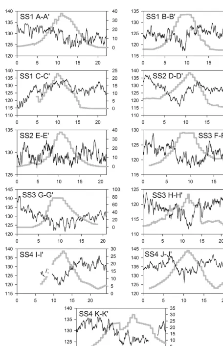
4.1. BRP over sticky spots using modelled attenuation We have generated BRP profiles for each flight section using the modelled attenuation correction described in Section 3.3.1. These results are plotted against the inferred basal drag in Figure 4. In most of the profiles the increase in basal drag associated with the sticky spot is accompanied by a local drop in BRP. The negative correlation is less clear in profiles C–C’ and E–E’.

4.2. Empirical englacial attenuation

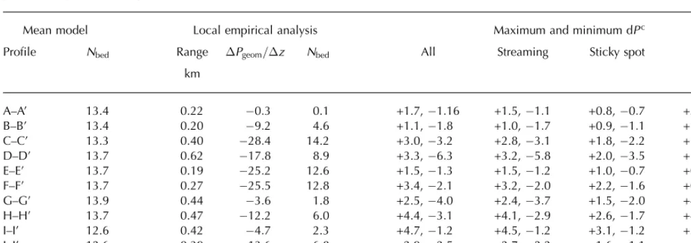
The Pgeom=z gradients are: for all survey points, 10:8 (over z range of 3.71 km); for streaming ice only, 11:8

Table 1.Comparison of englacial attenuation rates and BRP mismatch between modelled and empirical approaches after correction and

normalization. ‘Mean modelNbed’ is the depth-mean attenuation rate to bed using the modelled method. For the ‘Local empirical analysis’

‘Range’ is the range of ice thicknesses over which the regression was performed,Pgeom=zis the gradient of the regression andNbedis the

derived depth-mean attenuation rate to bed. The ‘Maximum and minimum dPc_{’ refers to the maximum and minimum over- and}

underestimate of BRP using differentPgeom=zgradients calculated with different data subsets (i.e. all data, streaming ice only, sticky-spot

profiles only, individual profiles only)

Mean model Local empirical analysis Maximum and minimum dPc

Profile Nbed Range Pgeom=z Nbed All Streaming Sticky spot Local

km

A–A’ 13.4 0.22 0:3 0.1 +1.7, 1:16 +1.5, 1:1 +0.8, 0:7 +3.2, 2:0

B–B’ 13.4 0.20 9:2 4.6 +1.1, 1:8 +1.0, 1:7 +0.9, 1:1 +1.2, 1:9

C–C’ 13.3 0.40 28:4 14.2 +3.0, 3:2 +2.8, 3:1 +1.8, 2:2 +1.1, 0:5

D–D’ 13.7 0.62 17:8 8.9 +3.3, 6:3 +3.2, 5:8 +2.0, 3:5 +1.9, +3.4

E–E’ 13.7 0.19 25:2 12.6 +1.5, 1:3 +1.5, 1:2 +1.0, 0:7 +0.3, 0:2

F–F’ 13.7 0.27 25:5 12.8 +3.4, 2:1 +3.2, 2:0 +2.2, 1:6 +0.9, 0:8

G–G’ 13.9 0.44 3:6 1.8 +2.5, 4:0 +2.4, 3:7 +1.5, 2:0 +4.0, 5:7

H–H’ 13.7 0.47 12:2 6.0 +4.4, 3:1 +4.1, 2:9 +2.6, 1:7 +4.0, 2:8

I–I’ 12.6 0.42 4:7 2.3 +4.7, 1:2 +4.5, 1:2 +3.1, 1:2 +5.8, 1:8

J–J’ 12.6 0.39 13:6 6.8 +2.9, 2:5 +2.7, 2:2 +1.6, 1:1 +2.4, 1:9

K–K’ 12.4 0.45 13:1 6.6 +1.2, 1:3 +1.1, 1:0 +1.7, 0:8 +1.1, 0:7

Ashmore and others: Ice-stream sticky spots and radar reflectivity

Fig. 4.Radar-recovered BRP using modelled attenuation (left-hand axis and black curve) plotted with satellite data and model-inverted basal drag (right-hand axis and heavy grey curve) over the 11 flight sections shown in Figure 3. Note that profiles G–G’, H–H’, J–J’ and K–K’ were

(z range of 2.45 km); sticky-spot profiles only, 17:5 (z

range of 1.40 km). The gradients derived from individual profiles are shown in Table 1. dPc _{values allow the} evaluation of BRP derived from empirical methods relative to the model-derived BRP. For profiles A–A’, B–B’, E–E’ (with one exception) and K–K0_{, empirical derivations of}

attenu-ation over- or underestimate the modelled BRP by <2 dB. We note that profiles A–A0_{, B–B}0 _{and E–E}0 _{are orientated}

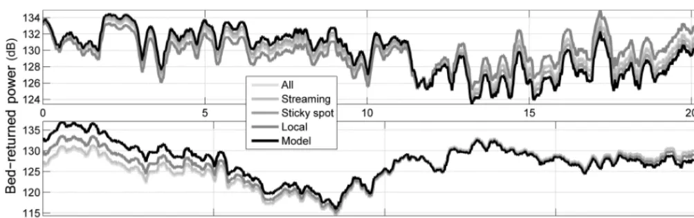
along flowlines in the lower ice stream and that this similarity is likely due to unchanging ice properties along-track. Most common are under- and overestimates of 3–5 dB, which are large enough to warrant interpretative caution. Using all the survey data or streaming data results in larger dPc _{values owing to the less-negative gradients of these} regressions, relative to those using the sticky-spot profiles. In some cases the locally derived rate (profiles C–C’, E–E’, F–F’) ofNbed is within 1 dB km–1of the model-derived rate, so dPc_{is small. However, in many cases dP}c_{is large enough to} be treated with caution, in particular profile G–G’ which has a dPc_{range of 9.7 dB. Example adjusted BRP profiles for A–} A’ and D–D’ are shown in Figure 5 and demonstrate that in some cases the along-track pattern of BRP is not preserved when using an empirical attenuation correction.

5. DISCUSSION

5.1. Potential sources of error

The interpretation of radar data in remote areas frequently cannot be validated with ground-based observations. Thus robust data interpretation must include an appraisal of potential errors, the most significant of which are likely to lie in the approach and assumptions used to estimate englacial attenuation.

5.1.1. Evaluation of attenuation methods

In this analysis we have used airborne radar data to show that, in this setting, using empirical methods to account for attenuation typically underestimates BRP relative to that which is derived using a modelling approach to attenuation. We have found that the derivation of attenuation using an empirical approach will produce highly varying values, depending on the choice and location of the radar profiles used to generate the empirical estimate. Our findings therefore support the extreme caution advised by Matsuoka

(2011) and MacGregor and others (2012) with regard to using the empirical approach to derive attenuation. It is necessary, however, to consider that the modelled approach has some limitations with regard to its input data. In this study we omit the uncertainty associated with the ice dielectric property values used in the attenuation model, owing to the paucity of measurements across Antarctica (MacGregor and others, 2007). This is justified here with the emphasis that our focus is on practical interpretation-driven analysis of BRP trends in short radar profiles, rather than the derivations of absolute reflectivity across the larger region.

There are, however, cases reported from elsewhere where the empirical approach can be appropriate, and where its use offers a more efficient alternative. For example, Gades and others (2000) used a profile on Siple Dome, where the ice is expected to be frozen to the bed, to derive attenuation rates in the adjacent stagnant ice streams. As attenuation is likely to be higher within stagnant ice streams, owing to the presence of warm, formerly streaming ice, any observed increase in BRP there is likely to be indicative of real changes at the ice/bed. Similarly, Fujita and others (2012) demonstrated that in slow-moving areas of East Antarctica a linear BRP/ice-thickness relation is found in cold-bedded areas, contrasting with a less straightforward relationship between the two in warm-bedded areas. We therefore advocate that the use of the empirical approach in estimating englacial attenuation is appropriate only for smaller areas with relatively unchanging internal properties. In this context, the empirical approach is unsuitable for estimating catchment-wide attenuation across EIS, which contains almost all major variants of ice flow, from slow-flowing and probably cold-based interior and inter-tributary regions, through a number of tributary onset regions to fast-flowing and probably warm-based tributaries and the main ice-stream trunk. It is, however, appropriate to derive local attenuation estimates for isolated analyses, provided that the ice properties and thickness do not change significantly along-track.

Using modelling rather than an empirical approach to obtain attenuation places reliance on model performance, driven in particular by the assumptions inherent within the model and the correctness of the model input. Geothermal flux and accumulation input fields are typically poorly constrained, so their effects on attenuation must be con-sidered. Continent-wide studies of modelled englacial

Fig. 5.A comparison between the BRP using a modelled attenuation correction (black) and BRP using an empirical attenuation correction

(shades of grey), after normalization (Pc

adj; Eqn (5)), for profiles A–A’ and D–D’.

Ashmore and others: Ice-stream sticky spots and radar reflectivity

attenuation have shown that, in some settings, uncertainties in geothermal flux can be problematic (Matsuoka and others, 2012). When basal ice is at pressure-melting point, as is the case here, errors in the geothermal flux will affect the derived melt rates but have only a minor effect on the temperature profile, from which the attenuation is derived. Errors in the accumulation field will affect the temperature profile, but mainly in the upper part of the ice column, where attenuation is relatively small. Differences between the true accumulation and that used as model input (Arthern and others, 2006) are probably systematic and occur on longer wavelengths than the features considered here. The steady-state model employed here does not account for transient ice temperature effects. We do not anticipate that transients are as likely in this region, given that the ice-stream tributaries are topographically confined. Moreover the slow-moving ice in this area contains well-preserved internal layering, a further indicator of its relative spatial ice-flow stability (Karlsson and others, 2012).

Our attenuation model accounts for the spatially varying effect of ice temperature but neglects the potential for spatially varying ice chemistry. Impurities in ice accumulate during snowfall (wet deposition) and from atmospheric fallout (dry deposition). There is some evidence that suggests an association between radar-active acidity and salinity with accumulation and elevation, respectively (Matsuoka and others, 2012). This potentially has significant implications in the Weddell Sea and Amundsen Sea sectors of West Antarctica, where high topography and accumu-lation coexist. However, this information remains based on a relatively small sample size and we take the view that, in the absence of more detailed parameterization of chemical variations across EIS, the better approach is not to introduce unknown complexity. A further consideration is that here we specifically limit ourselves to analysing relatively short (20 km) profiles in turn, along which we can assume that effects arising due to chemical variations are highly likely to be subordinate to those arising from temperature variation along-profile. We acknowledge, however, that further work is required to better understand the distribution of radar-active impurities on a variety of scales. Wolovick and others (2013) analysed the long (spatial) wavelength drift in high-amplitude anomalies to remove the cumulative effect of unconstrained power losses. This approach may prove useful in a larger analysis of the EIS dataset to evaluate systematic uncertainty in model-derived estimates of attenuation and BRP.

5.1.2. Additional sources of error

Radar energy can be directed away from the receiver by tilted internal layers and a strong bed slope. This effect is most apparent in profile J–J’ and is expressed as a strong negative excursion, 10 km along-track. This is the only profile associated with a steep bedrock step and the only profile which shows this feature. While topography varies in other profiles, it does so smoothly and the bed appears flat at the scale of a typical Fresnel zone (70 m in 2 km ice; Peters and others, 2005, their eqn (3)). Furthermore, the local drop in BRP occurs over a longer spatial scale than topographic features. Surface scattering losses (often induced by crevas-sing) are inferred to be important in airborne profiles across the Whillans Ice Stream shear margin (Peters and others, 2005). We do not cross any shear margins in the EIS profiles reported here and therefore do not anticipate similar losses.

5.2. Interpretation and potential significance of Evans Ice Stream sticky spots

As we reported in Section 1, there are several theories for the existence of sticky spots, ascribing the existence of these isolated areas of high basal drag beneath ice streams variously to notable protuberances of bedrock (i.e. sub-glacial mountains), exposure of bedrock from till drapes or variations in the wetness of till due to variations in basal ice temperature and/or subglacial hydrology (e.g. Alley, 1993; Stokes and others, 2007).

To our knowledge, evidence for the first of these possibilities has not been reported from any West Antarctic ice stream. Smith and others (2013) present seismic evidence from Pine Island Glacier of an area of high basal drag overlying a buried igneous intrusion, along with other sticky spots revealed by the inversion of inferometric synthetic aperture radar (InSAR) data (Joughin and others, 2009). Thus there is evidence from that site that sediment thinning can ultimately lead to the development of a ‘spot’ ‘sticky enough’ to retard ice flow. However, most of the reported examples of sticky spots in West Antarctica are in the Siple Coast ice streams, where they each represent patches of relatively dry or drying till (Alley, 1993; Sergienko and others, 2009; Winberry and others, 2011). The sticky spot beneath Kamb Ice Stream is clearly associated with a drop in radar BRP (Jacobel and others, 2009), and the existence of a dry bed there relative to the surrounding wet areas of the ice/bed interface has been confirmed with direct sampling (Engelhardt, 2004). Progres-sive dewatering of the till, perhaps over thinner till overlying a bedrock bump, has been proposed as the origin of this sticky spot which, once created, may have exerted sufficient basal drag to shut down Kamb Ice Stream150 years ago (Retzlaff and Bentley, 1993; Anandakrishnan and others, 2001; Jacobel and others, 2009).

additional consideration is that basal melt will, in theory, be elevated over the sticky spot, relative to the surrounding bed (Raymond, 2000; Sergienko and Hulbe, 2011). If this is the case, our BRP findings imply that any additional meltwater must be efficiently transported away from the sticky spot in a manner which keeps it relatively ‘dry’.

One important conclusion from this paper is that where sticky spots owe their existence to hydrological contrasts relative to the surrounding regions of ice-stream beds, they can be readily identified from radio-echo sounding surveys, providing that attenuation is appropriately constrained. Perhaps more importantly, however, our study has shown that sticky spots already identified as areas of high basal drag from inverting surface datasets (Joughin and others, 2006) have a corresponding physical explanation for their pres-ence at the bed. This gives confidpres-ence that surface data can be used to infer basal properties at appropriate scales of reference (De Rydt and others, 2013) and that output from such inversions is an appropriate first port-of-call in planning more targeted physical data acquisition from sticky spots when seeking more knowledge about their physical origins and evolution.

Interest in sticky spots is primarily driven by concerns over how they may disproportionately (for their size) affect the flow of major ice streams. The Kamb Ice Stream shutdown discussed above is perhaps the most extreme example. Sticky spots exerting significant resistance to the force balance of an ice stream have also been reported in Whillans Ice Stream (Winberry and others, 2011). Our study has highlighted that EIS and some of its tributaries are underlain by sticky spots, which, like those reported from Siple Coast ice streams, we have shown are more likely to be manifestations of patches of dewatered till. Hence their existence belies an organization of subglacial drainage through this catchment that keeps parts of the ice-stream/ tributary beds wet, while inducing a relative dewatering of other parts (i.e. the sticky spots). Understanding the processes by which such subglacial hydrological organ-ization has developed, and the timescales over which sticky spots are created, is therefore a crucial objective in constraining the future flow of this and other ice streams. In terms of the likely origins and evolution of the four sticky spots on EIS discussed in this paper, a key input to our inversions for basal drag was RADARSAT ice-velocity data from 1997 and 2000, whereas our radar data were acquired in 2006/07. The fact that both indicate sticky spots in consistent locations suggests that these features remained stable for at least the decade between these measurements. There is no evidence of large-scale subglacial-lake drainage in the EIS catchment (Smith and others, 2009), hence sticky-spot creation through that mode (Sergienko and Hulbe, 2011) seems unlikely here. Rather we suggest that the predominant influence here on any hydrological reorgan-ization is likely to be gradual changes in ice thickness and gradient with concomitant effects on basal temperature and subglacial water pressures. Current change across the EIS region is characterized by gradual ice thickening (Joughin and Bamber, 2005), while the grounding zone is very wide and subjected to a high tidal range (Gudmundsson, 2007; Sykes and others, 2009), making inland flow susceptible to tidal influences. Increased basal melt due to thicker ice would act to further decrease basal drag, if an inefficient drainage system is assumed. This scenario is reminiscent of the modern-day Whillans Ice Stream, where sticky-spot

processes modulate ice flow with a tidal periodicity (Winberry and others, 2011). If these processes continue, we hypothesize that EIS sticky spots may become similar influences on ice flow in the future. Targeting further data acquisition over these features in order to understand their physical origins and underlying processes is therefore an important scientific goal. Coincident seismic and radar acquisition along selected profiles, as undertaken by Murray and others (2008) across Rutford Ice Stream, offers promise as a mechanism for simultaneously obtaining the required information on till composition and wetness.

6. CONCLUSIONS AND OUTLOOK

We have analysed 1120 km radar profiles from Evans Ice Stream to show systematic variations of BRP in a warm-based ice-stream setting near inferred sticky spots. It is hypothesized that the local drop in BRP and coincident increase in basal drag we observe at several locations is due to areas of well-drained, thin or absent till relative to the surrounding area.

A long-standing aim of the glaciological community is to use radar reflectivity to distinguish between wet and dry ice-sheet beds, but this is hampered by the difficulty of reinstating losses from englacial attenuation. Model-focused studies have shown that traditional models of attenuation are limited and may lead to the misdiagnosis of bed conditions. We have tested these assertions by comparing two methods of accounting for englacial attenuation. We have confirmed the findings of model-based studies of englacial attenuation (Matsuoka, 2011; MacGregor and others, 2012) using field data, that empirical derivations of attenuation are unreliable without careful consideration of ice conditions and that a modelled approach is strongly favoured. Areas where particular care should be taken could be across ice-stream shear margins or where transient ice temperature effects are poorly known, such as stagnant ice streams where modelled and empirical methods may be found lacking.

Changes in sticky spots over time appear to lead to ice-stream flow dynamicism and are an under-represented feature in ice-sheet dynamic and prognostic models. They therefore represent key targets for further investigation, particularly where ice streams are underlain by thick, deformable layers of sediment, as is the case beneath EIS.

ACKNOWLEDGEMENTS

D.W.A. is supported by a University of Aberdeen College of Physical Sciences Studentship. Radar data were collected by the BAS as part of the IMAGE programme funded by the UK Natural Environment Research Council. The Scottish Alli-ance for Geosciences, Environment and Society (SAGES) and the Royal Astronomical Society provided funds which have advanced this work. Thanks are extended to scientific editor Sridhar Anandakrishnan, and two anonymous re-viewers for their constructive comments.

REFERENCES

Alley RB (1993) In search of ice-stream sticky spots. J. Glaciol.,

39(133), 447–454

Alley RB, Blankenship DD, Bentley CR and Rooney ST (1986) Deformation of till beneath Ice Stream B, West Antarctica.

Nature,322(6074), 57–59 (doi: 10.1038/322057a0)

Ashmore and others: Ice-stream sticky spots and radar reflectivity

Anandakrishnan S and Alley RB (1997) Tidal forcing of basal seismicity of Ice Stream C, West Antarctica, observed far

inland. J. Geophys. Res.,102(B7), 15 183–15 196 (doi: 10.1029/

97JB01073)

Anandakrishnan S, Alley RB, Jacobel RW and Conway H (2001) The flow regime of Ice Stream C and hypotheses concerning its

recent stagnation. In Alley RB and Bindschadler RA eds.The

West Antarctic ice sheet: behavior and environment. American Geophysical Union, Washington, DC, 283–296

Arthern RJ, Winebrenner DP and Vaughan DG (2006) Antarctic snow accumulation mapped using polarization of 4.3 cm

wavelength microwave emission. J. Geophys. Res.,111(D6),

D06107 (doi: 10.1029/2004JD005667)

Bindschadler R and 17 others (2011) Getting around Antarctica: new high-resolution mappings of the grounded and freely-floating boundaries of the Antarctic ice sheet created for the

International Polar Year. Cryosphere, 5(3), 569–588 (doi:

10.5194/tc-5-569-2011)

Bingham RG and 6 others (2012) Inland thinning of West Antarctic

Ice Sheet steered along subglacial rifts. Nature, 487(7408),

468–471 (doi: 10.1038/nature11292)

Blankenship DD, Bentley CR, Rooney ST and Alley RB (1986) Seismic measurements reveal a saturated porous layer beneath

an active Antarctic ice stream.Nature,322(6074), 54–57 (doi:

10.1038/322054a0)

Catania G, Hulbe C, Conway H, Scambos TA and Raymond CF (2012) Variability in the mass flux of the Ross ice streams, West

Antarctica, over the last millennium. J. Glaciol., 58(210),

741–752 (doi: 10.3189/2012JoG11J219)

Corr H and 8 others (2007) Airborne radio-echo sounding of the Wilkes Subglacial Basin, the Transantarctic Mountains, and the

Dome C region.Terra Antart. Rep.13, 55–64

De Rydt J, Gudmundsson GH, Corr HFJ and Christoffersen P (2013) Surface undulations of Antarctic ice streams tightly controlled by

bedrock topography.Cryosphere,7(2), 407–417 (doi: 10.5194/

tc-7-407-2013)

Engelhardt H (2004) Thermal regime and dynamics of the West

Antarctic ice sheet. Ann. Glaciol., 39, 85–92 (doi: 10.3189/

172756404781814203)

Fricker HA and Scambos T (2009) Connected subglacial lake activity on lower Mercer and Whillans Ice Streams, West

Antarctica, 2003–2008. J. Glaciol., 55(190), 303–315 (doi:

10.3189/002214309788608813)

Fujita S and 7 others (2012) Radar diagnosis of the subglacial

conditions in Dronning Maud Land, East Antarctica.Cryosphere,

6(5), 1203–1219 (doi: 10.5194/tc-6-1203-2012)

Gades AM, Raymond CF, Conway H and Jacobel RW (2000) Bed properties of Siple Dome and adjacent ice streams, West Antarctica, inferred from radio-echo sounding

measurements. J. Glaciol., 46(152), 88–94 (doi: 10.3189/

172756500781833467)

Gudmundsson GH (2007) Tides and the flow of Rutford Ice Stream,

West Antarctica. J. Geophys. Res., 112(F4), F04007 (doi:

10.1029/2006JF000731)

Gudmundsson GH (2011) Ice-stream response to ocean tides and

the form of the basal sliding law. Cryosphere, 5(1), 259–270

(doi: 10.5194/tc-5-259-2011)

Haran T, Bohlander J, Scambos T, Painter T and Fahnestock M (2006) MODIS mosaic of Antarctica (MOA) image map. National Snow and Ice Data Center, Boulder, CO. Digital media: http://nsidc.org/data/moa/

Hindmarsh RCA, Leysinger Vieli GJM and Parrenin F (2009) A

large-scale numerical model for computing isochrone geometry.Ann.

Glaciol.,50(51), 130–140 (doi: 10.3189/172756409789097450) Jacobel RW, Welch BC, Osterhouse D, Pettersson R and MacGregor JA (2009) Spatial variation of radar-derived basal conditions on

Kamb Ice Stream, West Antarctica.Ann. Glaciol.,50(51), 10–16

(doi: 10.3189/172756409789097504)

Jacobel RW, Lapo KE, Stamp JR, Youngblood BW, Welch BC and Bamber JL (2010) A comparison of basal reflectivity and ice

velocity in East Antarctica. Cryosphere, 4(4), 447–452 (doi:

10.5194/tc-4-447-2010)

Jones PC, Johnson AC, Von Frese RRB and Corr H (2002) Detecting rift basins in the Evans Ice Stream region of West Antarctica

using airborne gravity data. Tectonophysics, 347(1–3), 25–41

(doi: 10.1016/S0040-1951(01)00236-0)

Joughin I and Bamber JL (2005) Thickening of the ice stream catchments feeding the Filchner–Ronne Ice Shelf, Antarctica.

Geophys. Res. Lett., 32(17), L17503 (doi: 10.1029/ 2005GL023844)

Joughin I, Tulaczyk S, MacAyeal D and Engelhardt H (2004) Melting

and freezing beneath the Ross ice streams, Antarctica.J. Glaciol.,

50(168), 96–108 (doi: 10.3189/172756504781830295)

Joughin I, Bamber JL, Scambos T, Tulaczyk S, Fahnestock M and MacAyeal DR (2006) Integrating satellite observations with modelling: basal shear stress of the Filcher–Ronne ice streams,

Antarctica. Philos. Trans. R. Soc. London, Ser. A, 364(1844),

1795–1814 (doi: 10.1098/rsta.2006.1799)

Joughin I and 6 others (2009) Basal conditions for Pine Island and Thwaites Glaciers, West Antarctica, determined using satellite

and airborne data. J. Glaciol.,55(190), 245–257 (doi: 10.3189/

002214309788608705)

Karlsson NB, Rippin DM, Bingham RG and Vaughan DG (2012) A ‘continuity-index’ for assessing ice-sheet dynamics from

radar-sounded internal layers.Earth Planet. Sci. Lett.,335–336, 88–94

(doi: 10.1016/j.epsl.2012.04.034)

Langley K and 8 others (2011) Recovery Lakes, East Antarctica:

radar assessment of sub-glacial water extent. Geophys. Res.

Lett.,38(5), L05501 (doi: 10.1029/2010GL046094)

Leysinger Vieli GJMC, Hindmarsh RCA, Siegert MJ and Bo S (2011) Time-dependence of the spatial pattern of accumulation rate in East Antarctica deduced from isochronic radar layers using a

3-D numerical ice flow model. J. Geophys. Res.,116(F2), F02018

(doi: 10.1029/2010JF001785)

MacGregor JA, Winebrenner DP, Conway H, Matsuoka K, Mayewski PA and Clow GD (2007) Modeling englacial radar attenuation at Siple Dome, West Antarctica, using ice chemistry

and temperature data. J. Geophys. Res.,112(F3), F03008 (doi:

10.1029/2006JF000717)

MacGregor JA, Matsuoka K and Studinger M (2009) Radar

detection of accreted ice over Lake Vostok, Antarctica. Earth

Planet. Sci. Lett.,282(1–4), 222–233 (doi: 10.1016/j.epsl.2009. 03.018)

MacGregor JA, Matsuoka K, Waddington ED, Winebrenner DP and Pattyn F (2012) Spatial variation of englacial radar attenuation: modeling approach and application to the Vostok flowline.

J. Geophys. Res.,117(F3), F03022 (doi: 10.1029/2011JF002327) Matsuoka K (2011) Pitfalls in radar diagnosis of ice-sheet bed

conditions: lessons from englacial attenuation models.Geophys.

Res. Lett.,38(5), L05505 (doi: 10.1029/2010GL046205) Matsuoka K, Morse D and Raymond CF (2010) Estimating englacial

radar attenuation using depth profiles of the returned power,

central West Antarctica. J. Geophys. Res.,115(F2), F02012 (doi:

10.1029/2009JF001496)

Matsuoka K, MacGregor JA and Pattyn F (2012) Predicting radar

attenuation within the Antarctic ice sheet. Earth Planet. Sci.

Lett.,359–360, 173–183 (doi: 10.1016/j.epsl.2012.10.018) Murray T, Corr H, Forieri A and Smith AM (2008) Contrasts in

hydrology between regions of basal deformation and sliding beneath Rutford Ice Stream, West Antarctica, mapped using

radar and seismic data.Geophys. Res. Lett.,35(12), L12504 (doi:

10.1029/2008GL033681)

Peters ME, Blankenship DD and Morse DL (2005) Analysis techniques for coherent airborne radar sounding: application

to West Antarctic ice streams. J. Geophys. Res., 110(B6),

B06303 (doi: 10.1029/2004JB003222)

Raymond CF (2000) Energy balance of ice streams. J. Glaciol.,

46(155), 665–674 (doi: 10.3189/172756500781832701)

Stream, West Antarctica, and implications for margin processes.

J. Glaciol.,52(176), 3–10 (doi: 10.3189/172756506781828890) Retzlaff R and Bentley CR (1993) Timing of stagnation of Ice Stream C, West Antarctica, from short-pulse radar studies of buried

surface crevasses. J. Glaciol.,39(133), 553–561

Rignot E, Mouginot J and Scheuchl B (2011a) Ice flow of the

Antarctic Ice Sheet. Science, 333(6048), 1427–1430 (doi:

10.1126/science.1208336)

Rignot E, Mouginot J and Scheuchl B (2011b) Antarctic grounding line mapping from differential satellite radar interferometry.

Geophys. Res. Lett., 38(10), L10504 (doi: 10.1029/ 2011GL047109)

Rippin DM, Bamber JL, Siegert MJ, Vaughan DG and Corr HFJ (2006) Basal conditions beneath enhanced-flow tributaries of

Slessor Glacier, East Antarctica. J. Glaciol.,52(179), 481–490

(doi: 10.3189/172756506781828467)

Ross N and 9 others (2012) Steep reverse bed slope at the grounding line of the Weddell Sea sector in West Antarctica.

Nature Geosci.,5(6), 393–396 (doi: 10.1038/ngeo1468) Sergienko OV and Hulbe CL (2011) ‘Sticky spots’ and subglacial

lakes under ice streams of the Siple Coast, Antarctica. Ann.

Glaciol.,52(58), 18–22 (doi: 10.3189/172756411797252176) Sergienko O, MacAyeal DR and Bindschadler RA (2009) Stick–slip

behavior of ice streams: modeling investigations.Ann. Glaciol.,

50(52), 87–94 (doi: 10.3189/172756409789624274)

Smith AM and Murray T (2009) Bedform topography and basal conditions beneath a fast-flowing West Antarctic ice stream.

Quat. Sci. Rev., 28(7–8), 584–596 (doi: 10.1016/j.quascirev. 2008.05.010)

Smith AM, Jordan TA, Ferraccioli F and Bingham RG (2013) Influence of subglacial conditions on ice stream dynamics: seismic and potential field data from Pine Island Glacier, West

Antarctica. J. Geophys. Res., 118(B4), 1471–1482 (doi:

10.1029/2012JB009582)

Smith BE, Fricker HA, Joughin IR and Tulaczyk S (2009) An inventory of active subglacial lakes in Antarctica detected by

ICESat (2003–2008). J. Glaciol., 55(192), 573–595 (doi:

10.3189/002214309789470879)

Stokes CR, Clark CD, Lian OB and Tulaczyk S (2007) Ice stream sticky spots: a review of their identification and influence beneath contemporary and palaeo-ice streams.

Earth-Sci. Rev., 81(3–4), 217–249 (doi: 10.1016/j.earscirev. 2007.01.002)

Sykes HJ, Murray T and Luckman A (2009) The location of the grounding zone of the Evans Ice Stream, Antarctica, investigated

using SAR interferometry and modelling.Ann. Glaciol.,50(52),

35–40 (doi: 10.3189/172756409789624292)

Vaughan DG, Smith AM, Nath PC and Le Meur E (2003) Acoustic impedance and basal shear stress beneath four Antarctic ice

streams. Ann. Glaciol., 36, 225–232 (doi: 10.3189/

172756403781816437)

Vaughan DG, Corr HFJ, Smith AM, Pritchard HD and Shepherd A (2008) Flow-switching and water piracy between Rutford Ice

Stream and Carlson Inlet, West Antarctica. J. Glaciol.,54(184),

41–48 (doi: 10.3189/002214308784409125)

Wagman BM and Catania GA (2013) The impact of subglacial hydrology on the force balance of a physically modelled ice

stream. Ann. Glaciol., 54(63 Pt 2), 333–342 (doi: 10.3189/

2013AoG63A345)

Winberry JP, Anandakrishnan S, Wiens DA, Alley RB and Christianson K (2011) Dynamics of stick–slip motion, Whillans

Ice Stream, Antarctica. Earth Planet. Sci. Lett., 305(3–4),

283–289 (doi: 10.1016/j.epsl.2011.02.052)

Winebrenner DP, Smith BE, Catania GA, Conway HB and Raymond CF (2003) Radio-frequency attenuation beneath Siple Dome, West Antarctica, from wide-angle and profiling radar

obser-vations. Ann. Glaciol., 37, 226–232 (doi: 10.3189/

172756403781815483)

Wolovick MJ, Bell RE, Creyts TT and Frearson N (2013) Identifica-tion and control of subglacial water networks under Dome A,

Antarctica. J. Geophys. Res.,118(1), 140–154 (doi: 10.1029/

2012JF002555)

Ashmore and others: Ice-stream sticky spots and radar reflectivity