Contents
PREFACE xvii
1
A
Survey of Computer
2-2Graphics
2
Computer-Aided Design 2-3
Presentation Graphics 'I 2-4
Computer Art l 3 2-5
Entertainment 18
Education and Training 2 1
Visualization 25
Image Processing 3 2
Graphical User Interfaces 3 4
Overview of Graphics
2
systems
35
2-62-1 VideoDisplayDevices 36 2-7
Refresh Cathode-Ray Tubes 37
Raster-Scan Displays 40
Random-Scan Displays 41
Color CRT Monitors 42
Direct-View Storage Tubes
4.5
Flat-Panel Displays
45
Three-Dimensional Viewing Devices
49
Stereoscopic and Virtual-Reality Systems
Raster-Scan System!; Video Controller
Raster-Scan Display Processor Random-Scan Systems
Graphics Monitors and Workstations Input Devices
Keyboards Mouse
Trackball and Spaceball Joysticks
Data Glove Digitizers Image Scanners Touch Panels Light Pens Voice Systems Hard-Copy Devices Graphics Software
Coordinate Representations Graphics Functions
Software Standards PHIGS Workstations Summary
References Exercises
Contents
3
Outout Primitives
83
Points and Lines
Line-Drawing Algorithms
DDA Algorithm
Bresenham's Line Algorithm
Parallel Line Algorithms
Loading the Frame Buffer
Line Function
Circle-Generating Algorithms
Properties of Circles
Midpoint Circle Algorithm
Ellipse-Generating Algorithms
Properties of Ellipses
Midpoint Ellipse Algorithm
Other Curves
Conic Sections
Polynomials and Spline Curves
Parallel Curve Algorithms
Curve Functions
Pixel Addressing
and Object Geometry
Screen Grid Coordinates
Maintaining Geometric Properties
of Displayed Objects
Filled-Area Primitives
Scan-Line Polygon
Fill
Algorithm
Inside-Outside Tests
Scan-Line Fill of Curved Boundary
Areas
Boundary-Fill Algorithm
Flood-Fill
Algorithm
Fill-Area Functions
Cell Array
Character Generation
Summary
Applications
References
Exercises
Attributes
of
Output
Primitives
143
Line Attributes
Line Type
Line Width
Pen and Brush Options
Line Color
Curve Attributes
Color and Grayscale Levels
Color Tables
Grayscale
Area-Fill Attributes
Fill Styles
Pattern Fill
Soft Fill
Character Attributes
Text Attributes
Marker Attributes
Bundled Attributes
Bundled Line Attributes
Bundled Area-Fi Attributes
Bundled Text Attributes
Bundled Marker Attributes
Inquiry Functions
Antialiasing
Supersampling Straight Line
Segments
Contents
Area Sampling Straight Line 5-6 Aff ine Transformations 208
Segments 174 5-7 Transformation Functions 208
Filtering Techniques 174 5-8 Raster Methods for Transformations 210
Pixel Phasing 1 75
Summary 212
Compensating for Line lntensity
Differences 1
75
References 21 3Antialiasing Area Boundaries 1
76
Exercises 213Summary References Exercises
Two-Dimensional
180180
6
Viewing
21
6
6-1 The Viewing Pipeline
5
Two-Dimensional Geometric
Transformations
1 8 3
6-2 6-3 Viewing Coordinate Reference Frame Window-teviewport Coordinate Transformation 5-1 Basic TransformationsTranslation Rotation Scaling
5-2 Matrix Representations
and Homogeneous Coordinates 5-3 Composite Transformations
Translations Rotations Scalings
General Pivot-Point Rotation General Fixed-Point Scaling General Scaling Directions Concatenation Properties
General Composite Transformations and Computational Efficiency 5-4 Other Transformations
Reflection Shear
Two-Dimensional Wewing Functions Clipping Operations
Point Clipping Line Clipping
Cohen-Sutherland Line Clipping Liang-Barsky Line Clipping Nicholl-Lee-Nicholl Line Clipping Line Clipping Using Nonrectangular Clip Windows
Splitting Concave Polygons Polygon Clipping
Sutherland-Hodgernan Polygon Clipping
Weiler-Atherton Polygon Clipping Other Polygon-Clipping Algorithms Curve Clipping
Text Clipping Exterior Clipping Summary 5-5 Transformations Between Coordinate References
7
Structures
Modeling
and Hierarchical
250
7-1 Structure Concepts 250
Basic Structure Functions 250 Setting Structure Attributes 253
7-2 Editing Structures 254
Structure Lists and the Element
Pointer 255
Setting the Edit Mode 250
Inserting Structure Elements 256 Replacing Structure Elements 257 Deleting Structure Elements 257 Labeling Structure Elements 258 Copying Elements from One Structure
to Another 260
7-3 Basic Modeling Concepts 2 60
Mode1 Representations 261
Symbol Hierarchies 262
Modeling Packages. 263
7-4 Hierarchical Modeling
with Structures 265
Local Coordinates and Modeling
Transformations 265
Modeling Transformations 266
Structure Hierarchies 266
Summary 268
References 269
Exercises 2 69
Graphical User
Interfaces
8
Methods
and
Interactive lnput
271
8-1 The User Dialogue Windows and Icons
Accommodating Multiple Skill Levels
Consistency
Minimizing Memorization Backup and Error Handling Feed back
8-2 lnput of Graphical Data Logical Classification of Input Devices Locator Devices Stroke Devices String Devices Valuator Devices Choice Devices Pick Devices 8 - 3 lnput Functions
Input Modes Request Mode
Locator and Stroke Input
in
Request ModeString Input in Request Mode Valuator Input in Request Mode Choice lnput in Request Mode Pick Input in Request Mode Sample Mode
Event Mode
Concurrent Use of Input Modes 8-4 Initial Values for Input-Device
Parameters
8-5 lnteractive Picture-Construction Techniques
Basic Positioning Methods Constraints
Grids Gravity Field
Rubber-Band Methods Dragging
8-6 Virtual-Reality Environments 292 10-4
Summary 233
References 294
Exercises 294 10-5
10-6
9
Concepts
Three-Dimensional
296
9-1 Three-Dimensional Display Methods Parallel Projection
Perspective Projection Depth Cueing
Visible Line and Surface Identification
Surface Rendering
Exploded and Cutaway Views Three-Dimensional and Stereoscopic Views
9-2 Three-Dimensional Graphics
Packages 302
Three-Dimensional
10-1 Polygon Surfaces Polygon Tables Plane Equations Polygon Meshes
10-2 Curved Lines and Surfaces 10-3 Quadric Sutiaces
Sphere Ellipsoid Torus Superquadrics Superellipse Superellipsoid Blobby Objects Spline Representations
Interpolation and Approximation Splines Parametric Continuity Conditions Geometric Continuity Conditions Spline Specifications Cubic Spline Interpolation Methods
Natural Cubic Splines Hermite Interpolation Cardinal Splines
Kochanek-Bartels Splines Bezier Curves and Surfaces Bezier Curves
Properties of Bezier Curves Design Techniques Using Bezier Curves
Cubic E z i e r Curves Bezier Surfaces
B-Spline Curves and Surfaces B-Spline Curves
Uniform, Periodic B-Splines Cubic, Periodic €3-Splines Open, Uniform B-Splines Nonuniform 13-Splines B-Spline Surfaces Beta-Splines
Beta-Spline Continuity Conditions
Contents
Conversion Between Spline Representations
Displaying Spline Curves and Surfaces
Homer's Rule
Forward-Difference Calculations Subdivision Methods Sweep Representations Constructive Solid-Geometry Methods Octrees BSP Trees
Fractal-Geometry Methods Fractal-Generation Procedures Classification of Fractals Fractal Dimension Geometric Construction of Deterministic Self-Similar Fractals
Geometric Construction of Statistically Self-Similar Fractals
Affine Fractal-Construction Methods
Random Midpoint-Displacement Methods
Controlling Terrain Topography Self-squaring Fractals
Self-inverse Fractals Shape Grammars and Other Procedural Methods Particle Systems
Physically Based Modeling Visualization of Data Sets Visual Representations for Scalar Fields VisuaI Representations for Vector Fields Visual Representations for Tensor Fields
Visual Representations
for Multivariate Data Fields 402
Summary 4 0 4
References 404
Exercises 404
Three-Dimensional
11
Transformations
Geometric and Modeling
407
Translation 4 0 8
Rotation 409
Coordinate-Axes Rotations 409 General Three-Dimensional
Rotations 41 3
Rotations with Quaternions 419
Scaling 4 2 0
Other Transformat~ons 422
Reflections 422
Shears 423
Conlposite Transformations 423 Three-Dimens~onal Transformation
Functions 425
Modeling and Coordinate
Transformations 426
Summary 4 2 9
References 4 2 9
Exercises 4 3 0
Three-Dimensional
12
Viewing
4 3
1
12-1 Viewing Pipeline 4 3 2
12-2 Viewing Coordinates 4 3 3
Specifying the Virbw Plane 433 Transformation from World
- 40 1 to Viewing Coordinates 437
Contents
Projections
Parallel Projections Perspective IJrojections View Volumes and General Projection Transformations General Parallel-Projection Transformations General Perspective-Projection Transformations Clipping
Normalized View Volumes Viewport Clipping Clipping in Homogeneous Coordinates Hardware Implementations Three-Dimensional Viewing Functions Summary References Exercises
1 3-1 2 Wireframe Methods 490
13-1 3 Visibility-Detection Functions 490
Summary 49 1
Keferences 492
Exercises 49 2
lllumination
Models
14
and Surface-Rendering
Methods
494
Visi
ble-Su
dace Detection
Met
hods
469
Classification of Visible-Surface D~tection Algorithms
Back-Face Detection Depth-Buffer Method A-Buffer Method Scan-Line Method Depth-Sorting Method BSP-Tree Method Area-Subdivision Method Octree Methods
Ray-Casting Met hod Curved Surfaces
Curved-Surface Representations Surface Contour Plots
Light Sources
Basic lllumination Models Ambient Light
Diffuse Reflection Specular Reflection and the Phong Model
Combined Diffuse and Specular Reflections with Multiple Light Sources Warn Model Intensity Attenuation Color Considerations Transparency Shadows
Displaying Light Intensities Assigning Intensity Levels Gamma Correction and Video Lookup Tables
Displaying Continuous-Tone Images
Halftone Patterns and Dithering Techniques
Halftone Approximations Dithering Techniques Polygon-Rendering Methods Constant-Intensity Shading Gouraud Shading
Contents
Fast Phong Shading Ray-Tracing Methods Basic Ray-Tracing Algorithm Ray-Surface Intersection CaIculations
Reducing Object-Intersection Calculations
Space-Subdivision Methods AntiaIiased Ray Tracing Distributed Ray Tracing Radiosity Lighting Model Basic Radiosity Model Progressive Refinement Radiosity Method Environment Mapping Adding Surface Detail Modeling Surface Detail with Polygons
Texture Mapping Procedural Texturing Methods Bump Mapping Frame Mapping Summary References Exercises
15-6 CMY Color Model
15-7 HSV Color Model
15-8 Conversion Between HSV
and RGB Models
15-9 HLS Color Model
1 5-1 0 Color Selection and Applications Summary Reierences Exercises
16
Computer
Animation
583
14-1 Design of Animation Sequences
16-2 General Computer-Animation
Functions 16-3 Raster Animations
16-4 Computer-Animation Languages
16-5 Key-Frame Systems Morphing
Simulating Accelerations
16-6 Motion Specifications
Direct Motion Specification Goal-Directed Systems Kinematics and Dynamics
Color Models and Color
SummaryA p d
.
,ications
564
ReferencesExercises 597
15-1 Properties of Light 565
15-2 Standard Primaries and the
Chromaticity Diagram 568
A
Mathematics for Computer
XYZ Color Model 569
Graphics
599
CIE
Chromaticity Diagram569
A-1 Coordinate-Reference Frames 6 0 01 5-3 Intuitive Color Concepts 571 Two-Dimensional Cartesian
15-4 RGB Color Model
15-5 Y I Q Color Model
572 Reference Frames 600
5 74 Polar Coordinates in the xy Plane
601
Contents
Three-Dimensional Cartesian Reference Frames
Three-Dimensional Curvilinear Coordinate Systems
Solid Angle A-2 Points and Vectors
Vector Addition and Scalar Multiplication
Scalar Product of Two Vectors Vector Product of Two Vectors A-3 Basis Vectors and the Metric Tensor
Orthonormal Basis Metric Tensor A-4 Matrices
Matrix Transpose Determinant of a Matrix Matrix Inverse
Complex Numbers Quaternions
Nonparametric Representations Parametric Representations Numerical Methods
Solving
Sets
of Linear Equations Finding Roots of Nonlinear EquationsEvaluating Integrals Fitting C U N ~ S to Data Sets
Scalar Multiplication and Matrix
BIBLIOGRAPHY
Addition 612
Graphics
C
omputers have become a powerful tool for the rapid and economical pro- duction of pictures. There is virtually no area in which graphical displays cannot be used to some advantage, and so it is not surprising to find the use of computer graphics so widespread. Although early applications in engineering and science had to rely on expensive and cumbersome equipment, advances incomputer technology have made interactive computer graphics a practical tool. Today, we find computer graphics used routinely in such diverse areas as science, engineering, medicine, business, industry, government, art, entertainment, ad- vertising, education, and training. Figure 1-1 summarizes the many applications of graphics in simulations, education, and graph presentations. Before we get into the details of how to do computer graphics, we first take a short tour through a gallery of graphics applications.
-
F ' I ~ ~ I I ~ 1 - I
Examples of computer graphics applications. (Courtesy of DICOMED
A major use of computer graphics is in design processes, particularly for engi- neering and architectural systems, but almost all products are now computer de- signed. Generally referred to as CAD, computer-aided design methods are now routinely used in the design of buildings, automobiles, aircraft, watercraft, space- craft, computers, textiles, and many, many other products.
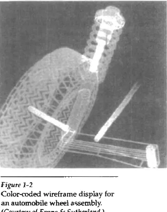
For some design applications; objeck are f&t displayed in a wireframe out- line form that shows the overall sham and internal features of obiects. Wireframe displays also allow designers to qui'ckly see the effects of interacthe adjustments to design shapes. Figures 1-2 and 1-3 give examples of wireframe displays in de- sign applications.
Software packages for CAD applications typically provide the designer with a multi-window environment, as in Figs. 1-4 and 1-5. The various displayed windows can show enlarged sections or different views of objects.
[image:14.527.198.369.360.577.2]Circuits such as the one shown in Fig. 1-5 and networks for comrnunica- tions, water supply, or other utilities a R constructed with repeated placement of a few graphical shapes. The shapes used in a design represent the different net- work or circuit components. Standard shapes for electrical, electronic, and logic circuits are often supplied by the design package. For other applications, a de- signer can create personalized symbols that are to be used to constmct the net- work or circuit. The system is then designed by successively placing components into the layout, with the graphics package automatically providing the connec- tions between components. This allows the designer t~ quickly try out alternate circuit schematics for minimizing the number of components or the space re-
-
quired for the system.Figure 1-2
Color-coded wireframe display for an automobile wheel assembly.
Figure 1-3
Color-coded wireframe displays of body designs for an aircraft and an automobile.
(Courtesy of (a) Ewns 6 Suthcrhnd and ( b ) Megatek Corporation.)
Animations are often used in CAD applications. Real-time animations using wiseframe displays on a video monitor are useful for testing perfonuance of a ve- hicle or system, as demonstrated in Fig. ld. When we do not display o b j s with rendered surfaces, the calculations for each segment of the animation can be per- formed quickly to produce a smooth real-time motion on the screen. Also, wire- frame displays allow the designer to see into the interior of the vehicle and to watch the behavior of inner components during motion. Animations in virtual-
reality environments are used to determine how vehicle operators are affected by
Figure 1-4
Multiple-window, color-coded CAD workstation displays. (Courtesy of Intergraph
Figure 1-5
A drcuitdesign application, using multiple windows and colorcded logic components, displayed on a Sun workstation with attached speaker and microphone. (Courtesy of Sun Microsystems.)
- . -
Figure 1-6
Simulation of vehicle performance during lane changes. (Courtesy of
Ewns 6 Sutherland and Mechanical
Dynrrrnics, lnc.)
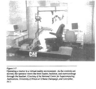
certain motions. As the tractor operator in Fig. 1-7 manipulates the controls,
the
headset presents a stereoscopic view (Fig. 1-8) of the front-loader bucket or the backhoe, just as if the operator were
in
the tractor seat. This allows the designer to explore various positions of the bucket or backhoe that might obstruct the o p erator's view, which can then be taken into account in the overall hactor design.Figure
1-9 shows a composite, wide-angle view from the tractor seat, displayed on a standard video monitor instead of in a virtual threedimensional scene.And
-
- - - - -
Figure 1-7
[image:17.527.82.415.60.369.2]Operating a tractor In a virtual-dty envimnment. As the contFols are moved, the operator views the front loader, backhoe, and surroundings through the headset. (Courtesy of the National Center
for Supercomputing
A p p l i c a t h , Univmity of Illinois at U r b a ~ C h r r m p i g n , and Catopillnr, Inc.)Figure 1-8
A headset view of the backhoe
presented to the tractor operator.
(Courtesy of the Notional Centerfor Supcomputing Applications, UniwrsifV of Illinois at Urbam- ~ h r r m p i & n d Caterpillnr, Inc.)
Figure 1-9
Operator's view of the tractor
bucket, cornposited in several
sections to form a wide-angle view
on a standard monitor. (Courtesy oi
Chapter 1 A Survey of Computer Graphics
Figure 1-10
View of the tractor displayed on a
standad monitor. (Courtesy of tk
National Cmter for Superwmputing ApplicPths, Uniwrsity of Illinois at
U r b P ~ U w m p i g n , and Gterpilhr, Inc.)
When obpd designs are complete, or nearly complete, realistic lighting models and surface rendering are applied to produce displays that wiU show the appearance of the final product. Examples of this are given in Fig. 1-11. Realistic displays are also generated for advertising of automobiles and other vehicles using special lighting effects and background scenes (Fig. 1-12).
The manufaduring process is also tied in to the computer description of d e signed objects to automate the construction of the product. A circuit board lay- out, for example, can be transformed into a description of the individud processes needed to construct the layout. Some mechanical parts are manufac-
tured by describing how the surfaces are to be formed with machine tools. Figure 1-13 shows the path to be taken by machine tools over the surfaces of an object during its construction. Numerically controlled machine tools are then set up to manufacture the part according to these construction layouts.
Figure 1-12
Studio lighting effects and realistic surfacerendering techniques are applied to produce advertising pieces for finished products. The data for this rendering of a Chrysler Laser was supplied by Chrysler Corporation. (Courtesy of Eric
Haines, 3DIEYE Inc. )
Figure 1-13
A CAD layout for describing the numerically controlled machining of a part. The part surface is displayed in one mlor and the tool
path in another color. (Courtesy of Los Alamm National Labomtoty.)
Figure 1-14
Chapter 1
A Survey of Computer Graphics
Architects use interactive graphics methods to lay out floor plans, such as Fig. 1-14, that show the positioning of rooms, doon, windows, stairs, shelves, counters, and other building features. Working from the display of a building layout on a video monitor, an electrical designer can try out arrangements for wiring, electrical outlets, and fire warning systems. Also, facility-layout packages can be applied to the layout to determine space utilization in an office or on a manufacturing floor.
Realistic displays of architectural designs, as in Fig. 1-15, permit both archi- tects and their clients to study the appearance of a single building or a group of buildings, such as a campus or industrial complex. With virtual-reality systems, designers can even go for a simulated "walk" through the rooms or around the outsides of buildings to better appreciate the overall effect of a particular design. In addition to realistic exterior building displays, architectural CAD packages also provide facilities for experimenting with three-dimensional interior layouts and lighting (Fig. 1-16).
Many other kinds of systems and products are designed using either gen- eral CAD packages or specially dweloped CAD software. Figure 1-17, for exam- ple, shows a rug pattern designed with a CAD system.
- Figrrre 1-15
Realistic, three-dimensional rmderings of building designs. (a) A street-level perspective for the World Trade Center project. (Courtesy of Skidmore, Owings & M m i l l . )
Figtin 1-16
A hotel corridor providing a sense of movement by placing light fixtures along an undulating path and creating a sense of enhy by using light towers at each hotel
room. (Courtesy of Skidmore, Owings
B Menill.)
Figure 1-17
Oriental rug pattern created with
computer graphics design methods.
(Courtesy of Lexidnta Corporation.)
.
-
PRESENTATION GRAPHICS
Another major applicatidn ama is presentation graphics, used to produce illus- trations for reports or to generate 35-mm slides or transparencies for use with projectors. Presentation graphics is commonly used to summarize financial, sta- tistical, mathematical, scientific, and economic data for research reports, manage rial reports, consumer information bulletins, and other
types
of reports. Worksta- tion devices and service bureaus exist for converting screen displays into 35-mm slides or overhead transparencies for use in presentations. Typical examples of presentation graphics are bar charts, line graphs, surface graphs, pie charts, and other displays showing relationships between multiple parametem.Figure 1-18 gives examples of two-dimensional graphics combined with g e ographical information.
This
illustration shows three colorcoded bar charts com- bined onto one graph and a pie chart with three sections. Similar graphs and charts can be displayed in three dimensions to provide additional information. Three-dimensional graphs are sometime used simply for effect; they can provide a more dramatic or more attractive presentation of data relationships. The charts in Fig. 1-19 include a three-dimensional bar graph and an exploded pie chart.Additional examples of three-dimensional graphs are shown in Figs. 1-20
Chapter 1
A SUN^^ of Computer Graph~s
Figure 1-18
Two-dimensional bar chart and me chart h k e d to a geographical c l h .
(Court~sy of Computer Assocbtes,
copyrighi 0 1992: All rights reserved.)
Figure 1-19
Three-dimensional bar chart. exploded pie chart, and line graph.
(Courtesy of Cmnputer Associates, copyi'ghi
6
1992: All rights reserved.)Figure 1-20
Showing relationships with a surface chart. (Courtesy of Computer
Associates, copyright O 1992. All rights reserved.)
Figure 1-21
Plotting two-dimensional contours in the &und plane, with a height field plotted as a surface above the
p u n d plane. (Cmrtesy of Computer
kclion 1-3
Computer Art
Figure 1-22
T i e chart displaying relevant information about p p c t tasks.
(Courtesy of computer Associntes,
copyright 0 1992. ,411 rights m d . )
Figure 1-22 illustrates a time chart used in task planning. Tine charts and task network layouts are used in project management to schedule and monitor the progess of propcts.
1-3
COMPUTER ART
Computer graphics methods are widely used in both fine art and commercial art applications. Artists use a variety of computer methods, including special-pur- p&e hardware, artist's paintbrush (such as Lumens), other paint pack- ages (such as Pixelpaint and Superpaint), specially developed software, symbolic mathematits packages (such as Mathematics), CAD paclpges, desktop publish- ing software, and animation packages that provide faciliHes for desigrung object shapes and specifiying object motions.
Figure 1-23 illustrates the basic idea behind a paintbrush program that al- lows artists to "paint" pictures on the screen of a video monitor. Actually, the pic- ture is usually painted electronically on a graphics tablet (digitizer) using a sty- lus, which can simulate different brush strokes, brush widths, and colors. A paintbrush program was used to m t e the characters in Fig. 1-24, who seem to be busy on a creation of their own.
A paintbrush system, with a Wacom cordlek, pressure-sensitive stylus, was used to produce the electronic painting in Fig. 1-25 that simulates the brush strokes of Van Gogh. The stylus transIates changing hand presswe into variable line widths, brush sizes, and color gradations. Figure 1-26 shows a watercolor painting produced with this stylus and with software that allows the artist to cre-
ate watercolor, pastel, or oil brush effects that simulate different drying out times, wetness, and footprint. Figure 1-27 gives an example of paintbrush methods combined with scanned images.
Figure 1-23
Cartoon drawing produced with a paintbrush program, symbolically illustrating an artist at work on a video monitor. (Courtesy of Gould Inc., Imaging 6 Graphics Division and Aurora
Imaging.)
plotter with specially designed software that can m a t e "automatic art" without intervention from the artist.
Figure 1-30 shows an example of "mathematical" art. This artist uses a corn- b i a t i o n of mathematical fundions, fractal procedures, Mathematics software, ink-jet printers, and other systems to create a variety of three-dimensional and two-dimensional shapes and stereoscopic image pairs. Another example of elm-
Figure 1-24
Cartoon demonstrations of an "artist" mating a picture with a paintbrush system. The picture, drawn on a graphics tablet, is displayed on the video monitor as the elves look on. In (b), the cartoon is superimposed
Figure 1-25
A Van Gogh look-alike created by graphcs artist E&abeth O'Rourke with a cordless, pressuresensitive stylus. (Courtesy of Wacom Technology Corpomtion.)
Figure 1-26
An elechPnic watercolor, painted by John Derry of Tune Arts, Inc. using a cordless, pressure-sensitive stylus and Lwnena gouache-brush &ware. (Courtesy
of
Wacom Technology Corporation.)Figure 1-27
The artist of this picture, called Electrunic Awlnnche, makes a statement
about our entanglement with technology using a personal computer with a graphics tablet and Lumena software to combine renderings of leaves, Bower petals, and electronics componenb with scanned images. (Courtesy of the Williams Gallery. w g h t 0 1991 by Imn Tnrckenbrod, Tke
Figwe 1-28 Figure 1-29
From a series called Sphnrs of Inpumce, this electronic painting Electronic art output to a pen (entitled, WhigmLaree) was awted with a combination of plotter from software specially methods using a graphics tablet, three-dimensional modeling, designed by the artist to emulate texture mapping, and a series of transformations. (Courtesy of the his style. The pen plotter includes
Williams Gallery. Copyn'sht (b 1992 by w n e RPgland,]r.) multiple pens and painting inshuments, including Chinese
brushes. (Courtesy of the Williams
Gallery. Copyright 8 by Roman
Vmtko, Minneapolis College of Art 6
Design.)
Figure 1-30
This creation is based on a visualization of Fermat's Last
Theorem, I"
+
y" = z", with n = 5, by Andrew Hanson,Department of Computer Science, Indiana University. The image
was rendered using Mathematics and Wavefront software. (Courtesy of the Williams Gallery. Copyright 8 1991 by Stcmrt
Dirkson.)
Figure 1-31
Using
mathematical hlnctiow, fractal procedures, and supermmpu ters, this artist-composer experiments with various designs to synthesii form and color with musical composition. (Courtesy
tronic art created with the aid of mathematical relationships is shown in Fig. 1-31. seaion 1-3
The artwork of this composer is often designed in relation to frequency varia- Computer Art tions and other parameters in a musical composition to produce a video that inte-
grates visual and aural patterns.
Although we have spent some time discussing current techniques for gen- erating electronic images in the fine arts, these methods are also applied in com- mercial art for logos and other designs, page layouts combining text and graph- ics, TV advertising spots, and other areas. A workstation for producing page layouts that combine text and graphics is ihstrated in Fig. 1-32.
For many applications of commercial art (and in motion pictures and other applications), photorealistic techniques are used to render images of a product. Figure 1-33 shows an example of logo design, and Fig. 1-34 gives three computer graphics images for product advertising. Animations are also usxi frequently in
advertising, and television commercials are produced frame by frame, where
l i p r t . 1-32
Page-layout workstation. (Courtesy oj Visunl Technology.)
Figure 1-33
Three-dimens~onal rendering for a
logo. (Courtesy of Vertigo Technology, Inc.)
- .
Fi<yuru 1
-
34Chapter 1 each frame of the motion is rendered and saved as an image file. In each succes- A Survey of Computer Graphics sive frame, the motion is simulated by moving o wpositions slightly from their positions in the previous frame. When all frames in the animation sequence have been mdered, the frames are t r a n s f e d to film or stored in a video buffer for playback. Film animations require 24 frames for each second in the animation se- quence. If the animation is to be played back on a video monitor, 30 frames per second are required.
A common graphics method employed in many commercials is rnorphing,
where one obiect is transformed (metamomhosed) into another. This method
has
been used in
h
commercials to an oii can into an automobile engine, an au- tomobile into a tiger, a puddle of water into a tk,and one person's face into an- other face. An example of rnorphing is given in Fig. 1-40.1-4
ENTERTAINMENT
Computer graphics methods am now commonly used in making motion pic- tures, music videos, and television shows. Sometimes the graphics scenes are dis-
played by themselves, and sometimes graphics objects are combined with the ac- tors and live scenes.
A graphics scene generated for the movie Star Trek-% Wrath of Khan is shown in Fig. 1-35. The planet and spaceship are drawn in wirefame form and will be shaded with rendering methods to produce solid surfaces. Figure 1-36 shows scenes generated with advanced modeling and surfacerendering meth- ods for two awardwinning short h.
Many
TV
series regularly employ computer graphics methods. Figure 1-37 shows a scene p d u c e d for the seriff Deep Space Nine. And Fig. 1-38 shows awireframe person combined with actors in a live scene for the series Stay lhned.
~ i a ~ h i a developed for the Paramount Pictures movie Stnr
In Fig. 1-39, we have a highly realistic image taken from a reconstruction of thir- M i o n 1-4 teenth-century Dadu (now Beijing) for a Japanese broadcast. Enterlainrnent
Music videos use graphin in several ways. Graphics objects can be com- bined with the live action, as in Fig.1-38, or graphics and image processing tech- niques can be used to produce a transformation of one person or object into an- other (morphing). An example of morphing is shown in the sequence of scenes in Fig. 1-40, produced for the David Byme video She's Mad.
F i p r c 1-36
(a) A computer-generated scene from the film M sD m m , copyright O Pixar 1987. (b) A computer-generated scene from the film K n i c M , copyright O Pixar 1989. (Courfesy of Pixar.)
- - - . - - -. - - -
I i p r c 1 - 17
A Survey of Computer Graphics
Figurp 1-38
Graphics combined with a Live scene in the TV series Stay 7bned.
(Courtesy of Rhythm 6 Hues Studios.)
Figure 1-39
An image from a &owhuction of thirteenth-centwy Dadu (Beijmg today), created by Taisei
Corporation (Tokyo) and rendered
St*ion 1-5
Education and Training
F i p w I -413
Examples of morphing from the David Byrne video Slw's Mnd. (Courtcsv of Dnvid Bvrne, I& video. o h ~ a c i f i c Dota
Images.)
1-5
EDUCATION AND TRAINING
Computer-generated models of physical, financial, and economic systems are often used as educational aids. Models of physical systems, physiological sys- tems, population trends, or equipment, such as the colorcoded diagram in Fig. 1-
41, can help trainees to understand the operation of the system.
For some training applications, special systems are designed. Examples of such specialized systems are the simulators for practice sessions or training of ship captains, aircraft pilots, heavy-equipment operators, and air trafficcontrol personnel. Some simulators have no video screens; for example, a flight simula- tor with only a control panel for instrument
flying.
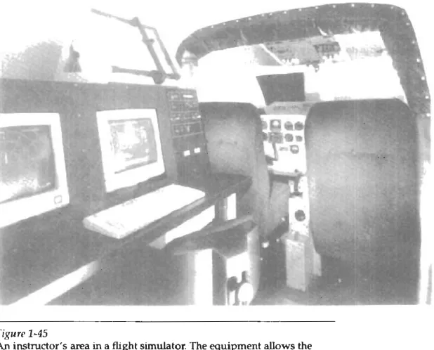
But most simulators provide graphics screens for visual operation. Two examples of large simulators with in- ternal viewing systems are shown in Figs. 1-42 and 1-43. Another type of viewing system is shown in Fig. 1 4 4 . Here a viewing screen with multiple panels is mounted in front of the simulator. and color projectors display the flight m e on the screen panels. Similar viewing systems are used in simulators for training air- craft control-tower personnel. Figure 1-45 gives an example of the inshuctor's area in a flight simulator. The keyboard is used to input parameters affeding the airplane performance or the environment, and the pen plotter is used to chart the path of the aircraft during a training session.Figure 1 -4 1
Color-coded diagram used to explain the operation of a nuclear reactor. (Courtesy of Las Almnos
National laboratory.)
Figure 1-42
A
Me,
enclosed tlight simulator with a full-color visual system andsix degrees of freedom in its motion. (Courtesy of F m x m
Intematwml.)
- --
Figure 1 4 3
kction 1-5
[image:33.527.53.467.65.266.2] [image:33.527.115.424.296.545.2]Edwtion and Training
Figure 1-44
A fight simulator with an external full-zulor viewing system. (Courtay a f F m
InternafiomI.)
Figure 1-45
F i p 1-46
Flightsimulator imagery. ((Courtesy
4
Emns 6 Sutherfund.) [image:34.527.261.444.350.546.2]-
Figure 1-47
Imagery generated for a naval
simulator. (Courtesy of Ewns 6 Sutherlrmd.)
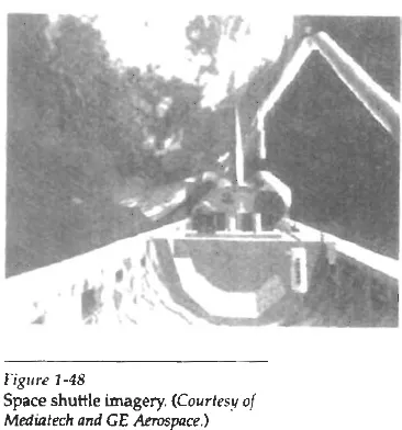
Figlire 1-48
Space shuttle imagery. (Courtesy of
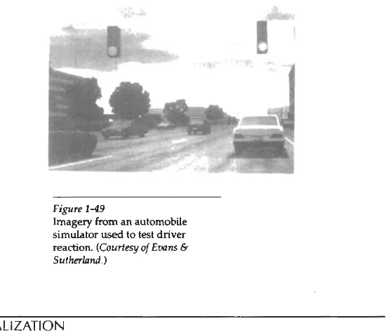
Figure 1-49
Imagery from an automobile
simulator used to test driver
reaction. (Courtesy of Evans 6 Sutherlrmd.)
1-6
VISUALIZATION
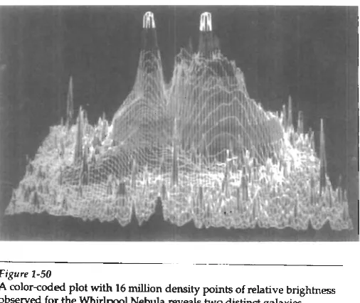
Scientists, engineers, medical personnel, business analysts, and others often need to analyze large amounts of information or to study the behavior of certain processes. Numerical simulations carried out on supercomputers frequently pro- duce data files containing thousands and even millions of data values. Similarly, satellite cameras and other sources are amassing large data files faster than they can be interpreted. Scanning these large sets of n u m b a to determine trends and relationships is a tedious and ineffective process. But if the data are converted to a visual form, the trends and patterns are often immediately apparent. Figure 1- 50 shows an example of a large data set that
has
been converted to a color-coded display of relative heights above a ground plane. Once we have plotted the den- sity values in this way, we can see easily the overall pattern of the data. Produc- ing graphical representations for scientific, engineering, and medical data setsand processes is generally referred to as scientific visualization. And the tenn busi-
ness visualization is used in connection with data sets related to commerce, indus- try, and other nonscientific areas.
There
are many different kinds of data sets, and effective visualization schemes depend o n the characteristics of the data. A collection of data can con- tain scalar values, vectors, higher-order tensors, or any combiytion of these data types. And data sets can be two-dimensional or threedimensional. Color coding is just one way to visualize a data set. Additional techniques include contour plots, graphs and charts, surface renderings, and visualizations of volume interi- ors. In addition, image processing techniques are combined with computer graphics to produce many of the data visualizations.Mathematicians, physical scientists, and others use visual techniques to an- alyze mathematical functions and processes or simply to produce interesting graphical representations. A color plot of mathematical curve functions is shown in Fig. 1-51, and a surface plot of a function is shown in Fig. 1-52. Fractal proce-
Chapter 1
A Survey of Computer Graphics
[image:36.527.124.377.97.310.2]- .- Figure 1-50
A color-coded plot with 16 million density points of relative brightness
o b ~ t ? ~ e d for the Whirlpool Nebula reveals two distinct galaxies. (Courtesy of Lar AIam National Laboratory.)
- -
Figure 1-51 Figurn 1-52
Mathematical curve functiow Lighting effects and surface- plotted in various color rendering techniqws were applied combinations. (Courtesy ofMeluin L. to produce this surface
Prun'tt, Los Alamos National representation for a three-
Laboratory.) dimensional funhon. (Courtesy of
dures using quaternions generated the object shown
in
Fig. 1-53, and a topologi- 1-6 cal shucture is displayed in Fig. 1-54. Scientists are also developing methods for wsualizationvisualizing general classes of data. Figure 1-55 shows a general technique for graphing and modeling data distributed over a spherical surface.
A few of the many other visualization applications
are
shown in Figs. 1-56 through 149.These
f i g k show airflow ove? ihe surface of a space shuttle, nu- merical modeling of thunderstorms, study of aack propagation in metals, acolorcoded plot of fluid density over an airfoil, a cross-sectional slicer for data sets, protein modeling, stereoscopic viewing of molecular structure, a model of the ocean floor, a Kuwaiti oil-fire simulation, an air-pollution study, a com-grow- ing study, rrconstruction of Arizona's Cham CanY& tuins, and a-graph ofauto- mobile accident statistics.
--
Figure 1-53
A four-dimensional object projected into three- dimensional space, then projected to a video monitor, and color coded. The obpct was generated using quaternions and fractal
squaring p r o c e d m , with an Want subtracted to show the complex Julia set. (Crmrtrsy of Iohn C. Ifart, School of Electrical Enginem'ng d
Computer Science, Washingfon State Uniwrsity.)
Figure 1 -54
Four views from a real-time, interactive computer-animation study of minimal surface ("snails") in the 3- sphere projected to three- dimensional Euclidean space. (Courtesy of George Francis, Deprtmmt of M a t h t i c s ad the Natwnal Colter for Sup~rromputing Applications, University of Illinois at UrhnaChampaign. Copyright O
1993.)
-
F+pre 1-55
Cjlapter 1 A Survey of Computer Graphics
Figure 1-56
A visualization of &eam surfaces
flowing past a space shuttle by Jeff
Hdtquist and Eric Raible, NASA
Ames. (Courtlsy
of
Sam W t o n , NASA Amcs Raaadr Cnrtlr.)Figure 1-57
Numerical model of airflow inside
a thunderstorm. (Cmtrtsv of Bob
Figure 2-58
Numerical model of the surface of a thunderstorm. (Courtsy of Sob
Wilklmsbn, Lkprhnmt of
Atmospheric Sciences and t k NatiaMl Center lor Supercomputing
--
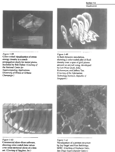
-- Figure 1-59C o l o r d e d visualization of stress energy density in a crack-
propagation study for metal plates, modeled by Bob Haber. (Courfesy of tk Natioml Cinter for
Supercaputmg Applicutions, U n m i t y of n l i ~ i s at Urbrmn-
Chnmpa~gn.)
Figure 1-60
A fluid dynamic simulation, showing a color-coded plot of fluid density over a span of grid planes around an aircraft wing, developed
by Lee-Hian Quek, John Eickerneyer, and Jeffery Tan.
(Courtesy of the Infinnation Technology Institute, Republic of Singapore.)
F@w 1-61
Commercial slicer-dicer software,
showing color-coded data values
over a w s e d i o n a l slices of a data
set. (Courtesy
of
Spyglnss, Im.)F i p m 1-62
Visualization of a protein structure
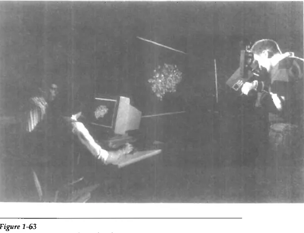
[image:39.527.77.472.72.592.2]Figure 1 -63
Stereoscopic viewing of a molecular strumup using a "boom" device.
(Courtesy of the N a f i a a l Centerfir Supermputing Applhtions, U n i v m i t y of Illinois at UrbomChnmprign.)
Figure 1-64
One image from a s t e n d q n c pair, showing a visualization of the ocean floor obtained from mteltik
data, by David Sandwell and
Chris
Small, Scripps Institution of Ocean- ography, and Jim Mdeod, SDSC.
(Courtesy of Stephanie Sids, Sun
Diego Supramrputer Center.)
Figvne 1 6 5
A simulation of the e f f d s of the Kuwaiti oil fire, by Gary Glatpneier, Chuck Hanson, and
Paul Hinker. ((Courtesy of Mike
Kmzh, Adrnnced Computing
lnboratwy 41 Los Alrrmos Nafionul
Section 1-6
Visualization
-1 ---7
-
[image:41.527.72.461.74.589.2]I
'1
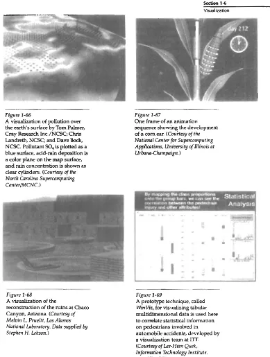
Figure 1-66
A visualization of pollution over the earth's surface by Tom Palmer,
Cray Research Inc./NCSC; Chris Landreth, NCSC; and Dave W,
NCSC. Pollutant SO, is plotted as a blue surface, acid-rain deposition is a color plane on the map surface, and rain concentration is shown as clear cylinders. (Courtesy
of
the North Cnmlim Supercomputing Center/MCNC.)- - . -
Figure 1-68
A visualization of the
reconstruction of the ruins at Cham Canyon, Arizona. (Courtesy of Melvin L. Pnceitt, Los Alamos
Nationul lnboratory. Data supplied by Stephen If. Lekson.)
Figure 1-67
One frame of an animation
sequence showing the development of a corn ear. (Couitcsy of tk National Center for Supmomputing Applimhs, U n i m i t y ofnlinois at UrhnaChampaign.)
Figure 1-69
A prototype technique, called WinVi, for visualizing tabular multidimensional data is used here to correlate statistical information on pedestrians involved in automobile accidents, developed by
Although methods used in computer graphics and Image processing overlap, the
amas am concerned with fundamentally different operations. In computer graphics, a computer is used to create a pichue. Image processing, on the other hand. applies techniques to modify or interpret existing pibures, such as p h e tographs and
TV
scans. Two principal applications of image pmcessing are (1) improving picture quality and (2) machine perception of visual information, as used in robotics.To apply imageprocessing methods, we first digitize a photograph or other picture into an image file. Then digital methods can be applied to rearrange pic- ture parts, to enhance color separations, or to improve the quality of shading. An
example of the application of imageprocessing methods to enhance the quality of a picture is shown in Fig. 1-70. These techniques are used extensively in com- mercial art applications that involve the retouching and rearranging of sections of photographs and other artwork. Similar methods are used to analyze satellite photos of the earth and photos of galaxies.
Medical applications also make extensive use of imageprocessing tech- niques for picture enhancements, in tomography and in simulations of opera- tions. Tomography is a technique of X-ray photography that allows cross-sec- tional views of physiological systems to be displayed. Both computed X-rav tomography (CT) and position emission tomography (PET) use propchon methods to reconstruct cross sections from digital data. These techniques are also used to
[image:42.527.195.407.350.565.2].- -.
figure 1-70
monitor internal functions and show crcss sections during surgery. Other me&
~~
1-7ical imaging techniques include ultrasonics and nudear medicine scanners. With Image Pm&ng ultrasonics, high-frequency sound waves, instead of X-rays, are used to generate
digital data. Nuclear medicine scanners colled di@tal data from radiation emit-
ted from ingested radionuclides and plot colorcoded images.
lmage processing and computer graphics are typically combined in
many applications. Medicine, for example, uses these techniques to model and study physical functions, to design artificial limbs, and to plan and practice surgery. The last application is generally referred to as computer-aided surgery.
[image:43.527.231.412.283.580.2]Two-dimensional cross sections of the body are obtained using imaging tech- niques. Then the slices are viewed and manipulated using graphics methods to simulate actual surgical procedures and to try out different surgical cuts.
Exam-
ples of these medical applications are shown in Figs. 1-71 and 1-72.Figure 1-71
One frame from a computer animation visualizing cardiac activation levels within regions of a semitransparent volume rendered dog heart. Medical data provided by Wiiam Smith, Ed Simpson, and G. Allan Johnson, Duke University. Image-rendering software by Tom Palmer, Cray Research, Inc./NCSC. (Courtesy of Dave Bock, North Carolina Supercomputing
CenterlMCNC.) Figure 1-72
One image from a stereoscopic pair showing the bones of a human hand. The images were rendered by lnmo Yoon, D. E. Thompson, and
W. N. Waggempack, Jr;, LSU, from a data set obtained with CT scans by Rehabilitation Research,
GWLNHDC. These images show a possible tendon path for
reconstructive surgery. (Courtesy of IMRLAB, Mechnniwl Engineering,
Chapter 1
1 4
ASuNe~ofComputerCraphics
GRAPHICAL USER INTERFACES
It is common now for software packages to provide a graphical interface. A major component of a graphical interface is a window manager that allows a user
.
to display multiple-window areas. Each window can contain a different process that can contain graphical or nongraphical displays. To make a particular win- dow active, we simply click in that window using an interactive pointing dcvicc.Interfaces also display menus and icons for fast selection of processing op- tions or parameter values. An icon is a graphical symbol that is designed to look like the processing option it represents. The advantages of icons are that they take u p less screen space than corresponding textual descriptions and they can be understood more quickly if well designed. Menbs contain lists of textual descrip- tions and icons.
Figure 1-73 illustrates a typical graphical mterface, containing a window manager, menu displays, and icons. In this example, the menus allow selection of processing options, color values, and graphics parameters. The icons represent options for painting, drawing, zooming, typing text strings, and other operations connected with picture construction.
--
Figure 1-73
A graphical user interface, showing
multiple window areas, menus, and
icons. (Courtmy
of Image-ln
[image:44.527.210.387.281.487.2]D
ue to the widespread recognition of the power and utility of computer graphics in virtually all fields, a broad range of graphics hardware and software systems is now available. Graphics capabilities for both two-dimen- sional and three-dimensional applications a x now common on general-purpose computers, including many hand-held calculators. With personal computers, we can use a wide variety of interactive input devices and graphics software pack- ages. For higherquality applications, we can choose from a number of sophisti- cated special-purpose graphics hardware systems and technologies. In this chap ter, we explore the basic features of graphics hardwa~e components and graphics software packages.2-1
VIDEO DISPLAY DEVICES
Typically, the primary output device in a graphics system is a video monitor (Fig. 2-1). The operation of most video monitors is based on the standard cathode-ray tube
(CRT)
design, but several other technologies exist and solid-state monitors may eventually predominate.- -- -
rig~rrr 2-1
Refresh Cathode-Ray Tubes
F i p m 2-2 illustrates the basic operation of,a CRT. A beam of electrons (cathode rays), emitted by an electron gun, passes through focusing and deflection systems that direct the beam toward specified positions on the p h o s p h o m t e d screen. The phosphor then emits a small spot of light at each position contacted by the electron beam. Because the light emitted by the phosphor fades very rapidly, some method is needed for maintaining the screen picture. One way to keep the phosphor glowing is to redraw the picture repeatedly by quickly directing the electron beam back over the same points. This type of display is called a refresh
CRT.
The primary components of an electron gun in a CRT are the heated metal cathode and a control grid (Fig. 2-31. Heat is supplied to the cathode by direding a current through a coil of wire, called the filament, inside the cylindrical cathode structure.
This
causes electrons to be ' k i l e d off" the hot cathode surface. In the vacuum inside the CRT envelope, the free, negatively charged electrons are then accelerated toward the phosphor coating by a high positive voltage. The acceler-Magnetic
Deflection Coils Phosphor-
Focusina Coated
Screen
Electron Beam Connector Elrnron a !. .'k
- - -
Figure 2-2
Basic design of a magneticdeflection CRT.
Focusing Cathode Anode
I
Electron Beam
Path
kction 2-1 V k h Display Devices
[image:47.527.64.340.280.531.2]-
Figure 2-3
Chapter 2 ating voltage can be generated with a positively charged metal coating on the in- overview of Graphics Systems side of the CRT envelope near the phosphor screen, or an accelerating anode can be used, as in Fig. 2-3. Sometimes the electron gun is built to contain the acceler- ating anode and focusing system within the same unit.
Intensity of the electron beam is controlled by setting voltage levels on the control grid, which is a metal cylinder that fits over the cathode. A high negative voltage applied to the control grid will shut off the beam by repelling eledrons and stopping them from passing through the small hole at the end of the control grid structure. A smaller negative voltage on the control grid simply decreases the number of electrons passing through. Since the amount of light emitted by the phosphor coating depends on the number of electrons striking the screen, w e control the brightness of a display by varying the voltage on the control grid. We specify the intensity level for individual screen positions with graphics software commands, as discussed in Chapter 3.
The focusing system in a CRT is needed to force the electron beam to con- verge into a small spot as it strikes the phosphor. Otherwise, the electrons would repel each other, and the beam would spread out as it approaches the screen. Fo- cusing is accomplished with either electric or magnetic fields. Electrostatic focus- ing is commonly used in television and computer graphics monitors. With elec- trostatic focusing, the elwtron beam passes through a positively charged metal cylinder that forms an electrostatic lens, as shown in Fig. 2-3. The action of the electrostatic lens fdcuses the electron beam at the center of the screen, in exactly the same way that an optical lens focuses a beam of hght at a particular focal dis- tance. Similar lens focusing effects can be accomplished with a magnetic field set up by a coil mounted around the outside of the CRT envelope. Magnetic lens fc- cusing produces the smallest spot size on the screen and is used in special- purpose devices.
Additional focusing hardware is used in high-precision systems to keep the beam in focus at all m npositions. The distance that thc electron beam must travel to different points on the screen varies because thc radius of curvature for most CRTs is greater than the distance from the focusing system to the screen center. Therefore, the electron beam will be focused properly only at the center o t the screen. As the beam moves to the outer edges of the screen, displayed images become blurred. To compensate for this, the system can adjust the focusing ac- cording to the screen position of the beam.
As with focusing, deflection of the electron beam can be controlled either with electric fields or with magnetic fields. Cathode-ray tubes are now commonl!. constructed with magnetic deflection coils mounted on the outside of the CRT envelope, as illustrated in Fig. 2-2. Two pairs of coils are used, with the coils in each pair mounted on opposite sides of the neck of the CRT envelope. One pair is
mounted on the top and bottom of the neck, and the other pair is mounted on opposite sides of the neck. The magnetic, field produced by each pair of coils re- sults in a transverse deflection force that is perpendicular both to the direction of the magnetic field and to the direction of travel of the electron beam. Horizontal deflection is accomplished with one pair of coils, and vertical deflection by the other pair. The proper deflection amounts are attained by adjusting the current through the coils. When electrostatic deflection is used, two pairs of parallel plates are mounted inside the CRT envelope. One pair oi plates is mounted hori- zontally to control the vertical deflection, and the other pair is mounted verticall!. to control horizontal deflection (Fig. 2-4).
Ven~cal Focusing Deflection
Connector Elr-,:wn ticr~zontal Beam
Pins Gun De!lection Plates
Figure 2-4
Electmstatic deflection of the electron beam in a CRT.
Phosphor- Coated Screen
Electron
phor coating, they are stopped and thek kinetic energy is absorbed by the phos- phor. Part of the beam energy is converted by friction into heat energy, and the remainder causes electrons in the phosphor atoms to move up to higher quan- tum-energy levels. After a short time, the "excited phosphor electrons begin dropping back to their stable ground state, giving u p their extra energy as small quantums of Light energy. What we see on the screen is the combined effect of all the electron light emissions: a glowing spot that quickly fades after all the excited phosphor electrons have returned to their ground energy level. The frequency (or color) of the light emitted by the phosphor is proportional to the energy differ- ence between the excited quantum state and the ground state.
Different h n d s of phosphors are available for use in a CRT. Besides color, a mapr difference between phosphors is their persistence: how long they continue to emit light (that is, have excited electrons returning to the ground state) after the CRT beam is removed. Persistence is defined as the time it takes the emitted light from the screen to decay to one-tenth of its original intensity. Lower- persistence phosphors require higher refresh rates to maintain a picture on the screen without flicker. A phosphor with low persistence is useful for animation; a high-persistence phosphor is useful for displaying highly complex, static pic- tures. Although some phosphors have a persistence greater than 1 second, graph- ics monitors are usually constructed with a persistence in the range from 10 to 60
microseconds.
Figure 2-5 shows the intensity distribution of a spot on the screen. The in- tensity is greatest at the center of
the
spot, and decreaws with a Gaussian distrib- ution out to the edges of the spot. This distribution corresponds to the m s s - sectional electron density distribution of the CRT beam. 'The maximum number of points that can be displayed without overlap on a
CRT
is referred to as the resolution. A more precise definition of m!ution is the number of points per centimeter that can be plotted horizontally and vertically, although it is often simply stated as the total number of points in each direction. Spot intensity has a Gaussian distribution (Fig. 2-5), so two adjacent spok will appear distinct as long as their separation is greater than the diameter at which each spot has an intensity of about 60 percent of that at the center of the spot. This overlap position is illustrated in Fig. 2-6. Spot size also depends on intensity. As more electrons are accelerated toward the phospher per second, the CRT beam diameter and the illuminated spot increase. In addition, the increased exci- tation energy tends to spread to neighboring phosphor atoms not directly in theFipn 2-5
Intensity distribution of an illuminated phosphor spot on