A Framework For Learning Scene Independent Edge Detection

(1)

Theses Thesis/Dissertation Collections

5-2014

A Framework For Learning Scene Independent

Edge Detection

Aaron J. Wilbee

Follow this and additional works at:http://scholarworks.rit.edu/theses

This Thesis is brought to you for free and open access by the Thesis/Dissertation Collections at RIT Scholar Works. It has been accepted for inclusion in Theses by an authorized administrator of RIT Scholar Works. For more information, please contactritscholarworks@rit.edu.

Recommended Citation

(2)

Edge Detection

by

Aaron J. Wilbee

A Thesis Submitted in Partial Fulfillment of the Requirements for the Degree of Master of Science

in Electrical and Microelectronic Engineering

Supervised by

Professor Dr. Ferat Sahin

Department of Electrical and Microelectronic Engineering Kate Gleason College of Engineering

Rochester Institute of Technology Rochester, New York

May 2014

Approved by:

Dr. Ferat Sahin, Professor

Thesis Advisor, Department of Electrical and Microelectronic Engineering

Dr. Eli Saber, Professor

Committee Member, Department of Electrical and Microelectronic Engineering

Dr. Mark A. Hopkins, Associate Professor

Committee Member, Department of Electrical and Microelectronic Engineering

Dr. Sohail A. Dianat, Professor

(3)

Rochester Institute of Technology Kate Gleason College of Engineering

Title:

A Framework For Learning Scene Independent Edge Detection

I, Aaron J. Wilbee, hereby grant permission to the Wallace Memorial Library to

repro-duce my thesis in whole or part.

Aaron J. Wilbee

(4)

Dedication

This work is dedicated to all those who have helped make it possible. My wife, Jessica,

who is ever by my side, my family who have always been there to support and inspire me,

(5)

Acknowledgments

There are many people who have made my journey through my scholastic career possible

and I would like to take this opportunity to thank them.

Dr. Ferat Sahin for his constant guidance and direction through my academic journey at

RIT.

Rochester Institute of Technology for providing the resources needed for me to explore

my passion

My peers and fellow research assistants at the Multi-Agent Biorobotics Laboratory for all

their support.

Ryan Bowen and Shitij Kumar for their aid in my undergraduate work as well as in this

thesis.

Ugur Sahin for his insight and guidance in research. For the rest not mentioned I thank

(6)

Abstract

A Framework For Learning Scene Independent Edge Detection

Aaron J. Wilbee

Supervising Professor: Dr. Ferat Sahin

In this work, a framework for a system which will intelligently assign an edge detection

filter to an image based on features taken from the image is introduced. The framework has

four parts: the learning stage, image feature extraction, training filter creation, and filter

selection training. Two prototypes systems of this framework are given. The learning stage

for these systems is the Berkeley Segmentation Database coupled with the Baddelay Delta

Metric. Feature extraction is performed using a GIST methodology which extracts color,

intensity, and orientation information. The set of image features are used as the input to

a single hidden layer feed forward neural network trained using back propagation. The

system trains against a set of linear cellular automata filters which are determined to best

solve the edge image according to the Baddelay Delta Metric. One system uses cellular

automata augmented with a fuzzy rule. The systems are trained and tested against the

images from the Berkeley Segmentation Database. The results from the testing indicate

that systems built on this framework can perform better than standard methods of edge

(7)

List of Contributions

Publications

• A.J. Wilbee,”A Framework for Intelligent Creation of Edge Detection Filters,”

sub-mitted toSystems, Man, and Cybernetics (SMC), Hong Kong, 2015.

Contributions

• Design of modular framework for diverse scene edge detection filter creation.

• Development of Fuzzy Cellular Automata implementation for framework

• Development of Linear Cellular Automata implementation for framework.

• Results verifying that edge detection filters are highly correlated to the scenes that

(8)

List of Tables

4.1 Airplane (3096): BDM Error from System Trained and Tested Against

Same Ground Truth Index, Neural Network Hidden Layer 100 Nodes . . . 63

4.2 Cumulative BDM Error: System Trained and Tested Against Same Ground Truth Index, Neural Network Hidden Layer 100 Nodes . . . 63

4.3 Cumulative BDM Error:System Trained and Tested Against Same Ground Truth Index, Neural Network Hidden Layer 25, 50, and 100 Nodes . . . 64

4.4 Performance of Images in Figure 4.4 using BDM . . . 64

4.5 Second Run: Cumulative BDM . . . 67

4.6 Second Run: Number of Images Each Method Performed Best On . . . 70

4.7 Example Images: Filter, BDM and Standard Method Comparison Data . . . 73

4.8 Images Both Prototype Systems Solve Best: Filter, BDM and Standard Method Comparison Data . . . 75

4.9 Comparison by Number of Images Each Method Performed Best On, 25 Hidden Layer Node Neural Network . . . 78

4.10 Comparison by Cumulative BDM, 25 Hidden Layer Node Neural Network . 78 4.11 Fuzzy System: Comparison of Neural Network Sizes by Image Performance 79 4.12 Fuzzy System: Comparison of Neural Network Sizes by Cumulative BDM . 79 4.13 Images That Do Well In All Systems With Filter and BDM for Comparison 79 4.14 Busy Non-Fuzzy Edge ImageBDM Comparison forEdge Images After a Single Application of the CA Filter and Five Applications . . . 81

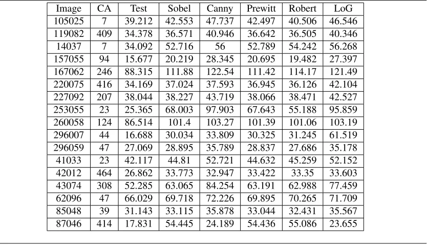
A.1 Individual BDM Error: Filter Selected by System Trained and Tested Against Ground Truth Index 1 . . . 98

B.1 BDM and Filters of Successful edge imagesFrom Non-Fuzzy System Us-ing 25 Hidden Nodes With Comparison BDM from Standard Methods . . . 107

B.2 Fuzzy System Filters Selected by Training Processes . . . 114

B.3 BDM and Filters of Successful edge imagesfrom Fuzzy System using 25 Hidden Nodes with Comparison BDM from Standard Methods . . . 115

(12)

C.2 Sparse Non-Fuzzy Run Successful Images with Filter and BDM for Com-parison . . . 130 C.3 Non-Fuzzy Run Successful Image for Both Systems with Filter and BDM

for Comparison . . . 130 C.4 Busy Fuzzy System: Filters Selected by Training Processes . . . 137 C.5 Busy Fuzzy System: Successful Images with Filter and BDM for Comparison137 C.6 Sparse Fuzzy System: Filters Selected by Training Processes . . . 138 C.7 Sparse Fuzzy System: Successful Images With Filter and BDM for

Com-parison . . . 139 C.8 Images Which Both Sparse and Busy Systems Solved Better Than Standard

(13)

List of Figures

2.1 Von Neumann and Moore Neighboorhoods . . . 6

2.2 Horizontal and Vertical Sobel Kernels . . . 14

2.3 Roberts Cross Filters . . . 16

2.4 Prewitt Filters . . . 16

2.5 Laplacian of Gaussian Filter . . . 17

2.6 Rule 250 [1] . . . 31

2.7 Rule 222 [2] . . . 31

2.8 Rule 30 [3] . . . 32

2.9 Rule 110 [4] . . . 32

2.10 PSO Algorithm . . . 35

2.11 Generalized Basic Neural Network Configuration . . . 37

2.12 Temperature Membership Functions . . . 38

3.1 Proposed Approach Block Diagram . . . 42

3.2 Example of Berkeley Data Set Image with Ground Truth, Snow Shoes (2018) 44 3.3 Three Feature Channel Scene Classification [5] . . . 48

3.4 Linear CA Neighborhood Inclusion Map . . . 50

3.5 Non-Fuzzy CA Neural Network . . . 57

3.6 Fuzzy CA Neural Network . . . 58

4.1 Airplane (3096) . . . 61

4.2 Airplane (3096): Ground Truths Index 1-5 . . . 61

4.3 Airplane (3906):Edge imagesSelected by Five Different Prototype Networks 63 4.4 Set Of Images For Which The Protoype System Selected Filter Outper-forms Standard Methods . . . 65

4.5 Confusion Matrix from Non-Fuzzy 25 Node Network Training . . . 68

4.6 Confusion Matrix from Fuzzy 25 Node Network Training . . . 69

4.7 Piglet (66053) . . . 73

4.8 Giraffe (253055) . . . 74

4.9 Kangaroo (69020) . . . 74

(14)

4.11 BillBoard (119082) . . . 75

4.12 Couple (157055) . . . 75

4.13 Wolf (167062) . . . 76

4.14 Cougar (42012) . . . 76

4.15 Wolf (167062) . . . 80

4.16 Fish (86068) . . . 80

4.17 Bright Stage . . . 83

4.18 Dim Stage . . . 84

4.19 cathedral (adsyiurcswacjxze) . . . 85

4.20 bookshelf (ajqdbufkmatgfhkx) . . . 86

A.1 105025 . . . 99

A.2 14037 . . . 99

A.3 157055 . . . 99

A.4 167062 . . . 100

A.5 220075 . . . 100

A.6 227092 . . . 101

A.7 253055 . . . 101

A.8 260058 . . . 102

A.9 296007 . . . 102

A.10 296059 . . . 102

A.11 306005 . . . 103

A.12 41033 . . . 103

A.13 42012 . . . 104

A.14 43074 . . . 104

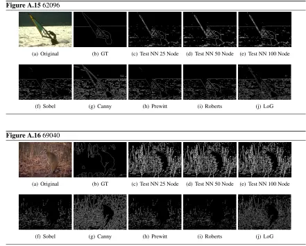
A.15 62096 . . . 105

A.16 69040 . . . 105

A.17 85048 . . . 106

A.18 86068 . . . 106

A.19 87046 . . . 106

B.1 Image 105025 . . . 108

B.2 Image 119082 . . . 108

B.3 Image 14037 . . . 108

B.4 Image 157055 . . . 109

B.5 Image 167062 . . . 109

(15)

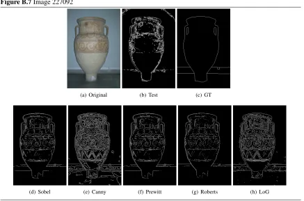
B.7 Image 227092 . . . 110

B.8 Image 253055 . . . 110

B.9 Image 260058 . . . 111

B.10 Image 296007 . . . 111

B.11 Image 296059 . . . 111

B.12 Image 41033 . . . 112

B.13 Image 42012 . . . 112

B.14 Image 43074 . . . 113

B.15 Image 62096 . . . 113

B.16 Image 85048 . . . 113

B.17 Image 87046 . . . 114

B.18 Image 103070 . . . 116

B.19 Image 119082 . . . 116

B.20 Image 12084 . . . 116

B.21 Image 130026 . . . 117

B.22 Image 145086 . . . 117

B.23 Image 147091 . . . 117

B.24 Image 148089 . . . 118

B.25 Image 157055 . . . 118

B.26 Image 16077 . . . 118

B.27 Image 163085 . . . 119

B.28 Image 167062 . . . 119

B.29 Image 175043 . . . 119

B.30 Image 189080 . . . 120

B.31 Image 210088 . . . 120

B.32 Image 236037 . . . 121

B.33 Image 253027 . . . 121

B.34 Image 253055 . . . 121

B.35 Image 304034 . . . 122

B.36 Image 306005 . . . 122

B.37 Image 3096 . . . 122

B.38 Image 33039 . . . 123

B.39 Image 38092 . . . 123

B.40 Image 42012 . . . 124

B.41 Image 66053 . . . 124

(16)

B.43 Image 8023 . . . 125

B.44 Image 86000 . . . 126

B.45 Image 86016 . . . 126

B.46 Image 86068 . . . 127

B.47 Image 89072 . . . 127

B.48 Image 97033 . . . 128

C.1 Images 101087 . . . 131

C.2 Images 123074 . . . 132

C.3 Images 167062 . . . 132

C.4 Images 253055 . . . 133

C.5 Images 260058 . . . 133

C.6 Images 41033 . . . 134

C.7 Images 43074 . . . 134

C.8 Images 62096 . . . 135

C.9 Images 86068 . . . 135

C.10 Images 42012 . . . 136

C.11 Images 108070 . . . 140

C.12 Images 108082 . . . 141

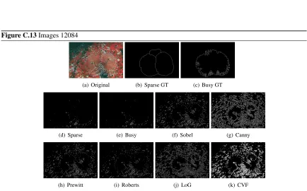
C.13 Images 12084 . . . 141

C.14 Images 14037 . . . 142

C.15 Images 167062 . . . 142

C.16 Images 196073 . . . 143

C.17 Images 304034 . . . 143

C.18 Images 69040 . . . 144

C.19 Images 8023 . . . 144

C.20 Images 86068 . . . 145

D.1 Image aaimforvxlklilzm . . . 146

D.2 Image adsyiurcswacjxze . . . 147

D.3 Image aikftgxhesyxsvwx . . . 148

D.4 Image aipzlmztzfaesuqi . . . 149

D.5 Image aajluizjalpcfwkf . . . 150

D.6 Image adqjafsbenxnqafr . . . 151

D.7 Image adubahgmhbvxcuuy . . . 152

D.8 Image aesyuxjawitlduic . . . 153

(17)

D.10 Image aameczztdzpctgas . . . 155

D.11 Image adcphrizvfpljiqt . . . 156

D.12 Image afpiqkoqucuomzrg . . . 157

D.13 Image ajijtsrervifddqo . . . 158

D.14 Image amjoyjrwhipnuvnm . . . 159

D.15 Image aeknnscdzemmcqji . . . 160

D.16 Image aitlekhnfcgheoar . . . 161

D.17 Image akpmyxoezscykphk . . . 162

D.18 Image aaulapocjffusovo . . . 163

D.19 Image aeswvtyqkhvasjui . . . 164

D.20 Image afqtsivgxsxbjlok . . . 165

D.21 Image adomfndhzlfgqlvx . . . 166

D.22 Image amrzytvcreqnwqmq . . . 167

D.23 Image apfiqqsakbuwpldm . . . 168

D.24 Image akyeueuomjjjgzrn . . . 169

D.25 Image amknzxaumkvwzfwh . . . 170

D.26 Image alybzdyjzdhkxeiw . . . 171

D.27 Image amkohsyogcolguzw . . . 172

D.28 Image actuxtkmvrrackkr . . . 173

D.29 Image atedeevhpbzyjtll . . . 174

D.30 Image ajqdbufkmatgfhkx . . . 175

D.31 Image altzsxfweazxvpbz . . . 176

D.32 Image arcklkvfquuqjhgc . . . 177

D.33 Image alizhxcsgtpjvrlz . . . 178

D.34 Image auxfadxjcaecurbm . . . 179

D.35 Image afliehgwaoiynwcw . . . 180

D.36 Image ajlvjxlreluvbtmn . . . 181

D.37 Image aanwybhpvpvtmrcr . . . 182

(18)

Chapter 1

Introduction

I

mage processing is a growing area of inquiry in electrical engineering with ever increasing

applications in both the public and private sectors. One sub-discipline which has grown out

of this field is computer vision. In computer vision, many tasks including image

segmenta-tion [6], background detecsegmenta-tion [7], and object detecsegmenta-tion [8] require that the contour of the

objects of interest be found. To succeed at this task the complete edge information of the

object must be detected. This thesis concerns the edge detection problem.

Edge detection is fascinating due to its nature as an ill posed problem; the true

defini-tion of an edge is unknown and the definidefini-tions used by humans are subjective [9]. Initial

research in this area has yielded a number of edge detectors which have come to be the

standard edge detection methods: Sobel, Canny, Prewitt, Roberts, and Laplacian of

Gaus-sian. These detectors define an edge as a high frequency change in an image [10]. These

methods, particularly Canny, yield goodedge imagesin many cases which is why they are

standards in many image processing tool boxes [11]. However there are many instances

where this definition of an edge is incorrect. A basic example would be the fur of an

ani-mal. In many images fur will have many high frequency changes. When a person is asked

(19)

in. In addition, noise in an image is also a high frequency change, but is rarely an edge. To

handle these issues the standard methods have the ability to adjust parameters to specialize

for the situations. The danger of specializing to a specific situation is that the same filter

will then perform worse in all other situations. In addition, because images are discrete

and noisy systems it is challenging to specialize these standard methods by hand to all the

necessary situations. Thus, as research has progressed, efforts at tuning definition based

edge detectors have shifted to machine learning approaches [11].

Rather than explicitly defining an edge, researchers have been attempting to train edge

detectors, which are suited to particular types of edges and images thus allowing the

com-puter to learn the edge definition. This is done by extracting features from the images to

train against. Many approaches using features, texture gradients and spectral clustering to

name a few, have been used to train these edge detectors. The features, once extracted,

are used in a learning algorithm such as: neural networks, genetic algorithms, and particle

swarm optimization. The learning algorithm is then used to create a new edge detector. The

limitation which arises when employing these methods is their lack of universality. Though

the filter, or set of filters, produced by this type of approach will work better than standard

methods for a particular class of images, they are observed to behave erratically outside of

that image type.

For many applications, this trade offis unimportant, the fields of: manufacturing, fault

detection, and security being a few examples. For these applications the environment is

typically highly controlled and known beforehand. As such, a specialized method for edge

(20)

beforehand, specialized edge detection begins to encounter issues. Specifically, the images

which have the properties that the edge detection method are expecting, have their edge

in-formation extracted well. However, for images with different properties the same methods

will perform poorly. For applications in mobile robotics and photography, this situation is

unacceptable. It is for this reason that this limitation of edge detection is being investigated

in this thesis.

The two current methods for edge detection, using a definition to produce an edge

de-tector or using features to train an edge dede-tector, both yield unsatisfactory results when

applied to a wide range of environments or scenes. The best solution to this problem would

be to find the universally correct definition of an edge and from there a universally correct

edge detector could be developed. However, this does not seem possible given the current

level of understanding and knowledge in the field. The approach which this thesis will

take is an extension of the training approach. Rather than creating a single filter, or set of

filters, which will solve a particular type of image, a framework for creating or matching

specialized filters to particular scenes will be created.

In this thesis a framework is developed for creating a system which will match an input

image with its corresponding edge filter. A system based on this framework will perform

better than current standard methods across a wide range of images from different

environ-ments or scenes.

The remainder of this document is organized as follows: Chapter 2 describes the

back-ground concepts necessary to understand and carry out the system outlined in this work.

(21)

into detail explaining each individual component. The explanation of each component is in

two parts: first the purpose of the component and what type of methodology can be used

to fulfill it is described, and then the particular approach to be used for the prototype

sys-tems is given. The results of the prototype Edge Filter Creation Syssys-tems are then given and

compared to other edge detection methods in Chapter 4. Conclusions are drawn in Chapter

(22)

Chapter 2

Background

This section is intended to give the background information needed to understand this

re-search’s proposed method and subsequent results.

2.1

Image Processing

Image processing is a discipline of signal processing. It is considered to be any

method-ology which takes as its input an image and returns a modified version of that image or a

set of features from the image or both. This research is focused on the creation of an edge

detection system. This is a fundamental image processing concept were the edges in an

image are determined using features from the image itself and are output as a

monochro-matic image containing only the edges. The remainder of this section will outline image

processing concepts related to this research.

2.1.1 Neighborhoods

In the context of image processing a neighborhood is the collection of pixels which is

considered when evaluating the next state of a pixel of interest. The two most common

neighborhoods, Von Neuman and Moore, are given by Figure 2.1. A Von Neumann

neigh-borhood has the pixel of interest at its center and the neighbors are considered to be

(23)

the pixel of interest at the center and the neighbors are considered to be every pixel that

shares an edge or a corner with the pixel of interest. Many other neighborhoods exist, each

used for different purposes under different circumstances. This research is concerned with

neighborhoods containing only in a 3x3 pixel neighborhood.

Figure 2.1Von Neumann and Moore Neighboorhoods

(a) Von Neuman Neighborhood (b) Moore Neighborhood

X gives the absolute position, Z gives the neighborhood position, relative to the pixel of interest

When dealing with neighborhoods it is important to consider what occurs when the

pixel of interest is at an edge of the image. These pixels are calledextreme pixels. For an

extreme pixel, a number of the pixels in its’ neighborhood extend offof the image which

render any operation depending on those pixels invalid. There are two primary approaches

for dealing with this occurrence. The first is known as a null boundary (NB) solution. This

solution simply assigns each neighborhood value which has extended offof the Image to

be 0. This is equivalent to zero padding the entire image so as to make every extreme pixel

have a valid neighborhood. The other solution is called a periodic boundary (PB). This type

of boundary assumes that the extreme pixels on each side are adjacent to each other. For

example: if the extreme pixel of interest was (3,0) then the pixel (3,-1) would be pixel (3,

(24)

2.1.2 Edge ImageCharacterization

A hard problem in edge detection is determining how good an edge image is. This is a

necessary evaluation, without it it would be impossible to determine if one edge detection

method was superior to another. Being able to rate edge detectors is particularly important

when training them because a fitness function is needed.

The place to start on this problem deciding what constitutes a goodedge image. Canny

gave one of the early definitions [13].

• Good detection: There should be a low probability of false negatives and false

posi-tives. This maximizes the signal to noise ratio.

• Good Localization: The marked edge should be as close as possible to the center of

the true edge to be detected.

• Single response: There should be only one edge pixel detected for every true edge

pixel that exists.

From this definition a number of methods for evaluatingedge imageshave been

devel-oped. The current methods foredge imagecharacterization can beneficially separated into

three types of methods: non-reference based measures, human evaluation, and reference

based measures. Non-reference based measures typically suffer from many biases and do

not use much information from the original image and as such will not be considered.

Hu-man evaluation, though more reliable than non-reference based measures, is impractical

because it is often challenging to use for an automation application [14]. In order to allow

(25)

for development and evaluation with human evaluation used only to supplement in the final

analysis.

Reference based methods use a gold standard or ground truth (GT) to compare generated

edge images against. At their core these methods are concerned with only two types of

fundamental errors. Type I errors are false positive edge pixels (FP), pixels which are

marked as edges by the detector but are not edge pixels according to the ground truth. Type

II errors are false negative edge pixels (FN), pixels which are marked as edge pixels in the

ground truth but not by the edge detector [15]. The remainder of this section will give an

overview of a few of the methods that have been used.

HausdorffMetric

The Hausdorffmetric is given by equation 2.1 and essentially gives the maximum distance

between an estimated pixel and its corresponding edge. The smaller the number the better

the images match. Though neither this author nor Baddeley have been able to find reference

of its use foredge imagecomparison it is interesting for a theoretical basis [15].

H(A,B)= maxsupx∈Ad(x,B),supx∈Bd(x,A) (2.1)

• Ais the Ground Truth Image with edge pixels marked as 1

• Bis the calculatededge imagewith edge pixels marked as 1

(26)

Misclassification Error Rate

Misclassification error rate is the simplest of the error metrics. It is the summation of all

of the type I and type II errors in theedge imagenormalized relative to the total number of

pixels [15] as given by equation 2.2. Simply stated it is the fraction of misclassified pixels.

This metric also indicates better performance with a lower score.

(A,B)= n(A∆B)

n(X) (2.2)

• Ais the ground truthedge image

• Bis the calculatededge image

• Xis the image itself

• nrepresents number of pixels in the set

Pratts Figure of Merit

Pratts Figure of Merit (FOM) is the most commonly used and accepted standard for edge

imageevaluation. It is given be equation 2.3. This equation attempts to assign an intelligent

error rating to the number of type I and II errors as well as address the localization problem

[16]. This metric gives a rating between 0 and 1, 1 being the best.

R= 1

IN

ΣIA i=1

1 1+a∗d2

1

(2.3)

• IN = MAXII,IA

(27)

– IA is the number of actualedge imagepixels

• ais a scaling constant which is adjusted to penalize lack of localization

• d1 is the distance between a predicted edge point and the nearest ground truth edge

point measured along a line normal to the nearest line of ground truth edge points.

From this single method there have been a number of improvements all of which report

results in the same way. One well known weakness of the FOM is that it does not

ade-quately account for type II errors. In particular, the location of the error pixel with respect

to the true edge is not taken into account. This causes unfair error in otherwise successful

images. Pinho et al. gives an extension to compensate for this discrepancy in equation 2.4,

note the definition ofdchanges [17].

R= 1

NT

ΣNT i=1

1 1+a∗d2

2

1

1+ β∗NF M NT

(2.4)

• NT is the number of ground truth edge pixels

• ais a scaling constant which is adjusted to penalize lack of localization

• d2 is the distance between a ground truth edge point and the nearest predicted edge

point.

• NF M is the number of false positive points

• βis the scaling factor for the false positive edges.

A further modification of that method was given by Wenlong et al. on the rationale that

(28)

d2, see equation 2.5 [16].

R= 1

NT∪P

ΣNT∪P i=1

1

(1+a∗d2₎₍₁+_a_∗_d2 2)

(2.5)

• NT∪P is the number of predicted of truth edge pixels.

Baddeley Delta Metric

The Baddeley Delta Metric (BDM) is a separate approach to correct a number of

weak-nesses in the FOM as well as other method of edge image comparison [15]. The

com-parison is accomplished in this method by measuring the similarity of subsets of featured

points, typically represented by the value 1. The measure adaptation for binary edge

im-agesis taken from a paper written by Uguz et al. [18]. For this measure the lower the score

the better theedge image.

Let B1 and B2 be two binary images with the same dimensions M × N, and let Ω =

{1, ...,M} × {1, ...,N} be the set of their positions. Given a value 1 < k < ∞ thek-BDM

between the images B1andB2(denotedΠk(B1,B2)) is defined as: [18]

Πk

(B1,B2)= [

1 |Ω|

X

t∈Ω

|w(d(t,B1)−w(d(t,B2)|]

1

k (2.6)

• d(t,Bi) is the Euclidean distance from the position tto the closest true edge featured

point of the image.

• Bi andw: [0,∞]→[0,∞]: A concave, increasing weighting function

• w(x)= x

(29)

These are but a few of the related methods for edge detection classification, many others

exist [9] [19] [20] [14].

This research uses the BDM. This metric was developed in order to improve upon other

existing methods, specifically Pratts Figure of Merit, misclassification error rate, and the

Hausdorffmetric. Baddeley gives very thorough reasoning as to how each of these metrics

are limited and how the BDM overcomes their limitations. The largest limitation to

con-sider is that of the FOM. The limitation of the FOM is its inability to handle localization

errors in any manner other than adjusting a scaling factor [15]. Essentially, the FOM does

not have the capacity to address the pattern of the error but only the average displacement

or the edge pixels from the anticipated ground truth positions. The Hausdorffmetric cannot

be used because it only gives the maximum error pixel and hence only needs one outlier to

skew the image results. The misclassification error rate is not useful for an edge detection

application because it does not concern itself with how close the error pixels are to correct,

only that they are errors.

2.1.3 Standard Edge Detection Methods

Edge detection is a fundamental problem in image processing, one which many other

tech-niques rely upon in order to function properly. As such, a great deal of research has been

done on edge detection are over the last few decades. Of the many approaches that have

been developed, there are a few which have emerged as the ’standard approaches’ for the

edge detection problem. These approaches work well in most instances: Sobal, Canny,

(30)

differential gradient of the image intensity. The following sections summarize these

tech-niques.

Sobel

This filter is named for Irwin Sobel. It is comprised of two orthogonal filters given by

Fig-ure 2.2. These filters are convolved with the original image resulting in an approximation

of the image intensity gradient for two orientations. These orientations are typically 0 and

90 degrees. The two resulting images from the convolution are overlaid to give a finaledge

image. This process is summarized in equation 2.7 [10].

Of =

q

g2

x +g2y

Of = p[(z7+2z8+z9)−(z1+2z2+z3)]2+[(z3+2z6+z9)−(z1+2z4+z7)]2

(2.7)

•

g

: Neighborhood to be convoluted against (kernel)

•

z

: Neighborhood location

•

O

f

: Resulting intensity gradient image

If a monochromatic image is required a thresholdT is then used on the finaledge image

to separate edge pixels from non-edge pixels as in equation 2.8.

(31)

Figure 2.2Horizontal and Vertical Sobel Kernels

(a) Horizontal (b) Vertical

Canny

The Canny filter is a methodology which builds on the Sobel filter by incorporating some

pre and post processing steps to increaseedge imagedetection accuracy. The Canny edge

detection approach is accomplished in 5 general steps [10].

• Image Smoothing: Typically accomplished using a two dimensional Gaussian filter

as in equation 2.1.3.

• Intensity Gradient: The Intensity Gradient is determined by convolving a Kernel

similar to the Sobel filter in Figure 2.2.

• Suppression Weak Edge Elimination: Because of the nature of the gradient

detec-tion, it is often the case that a given edge will be found to have a width of greater

than one pixel which is not ideal as mentioned in Section 2.1.2. The local maximum

gradient value in a given direction in a group of edge pixels is assigning to be the edge

pixel. This allows for edges of single pixel width to be created.

(32)

edges based on two intensity threshold.

• Track Edges: Weak edge pixels are included using heuristics to complete strong

edges.

G(x,y)=e

−x

2+_y2

2δ2 _(2.9)

Roberts

The Roberts filter, also known as the Roberts cross, accomplishes edge detection by taking

a discrete differentiation of a localized neighborhood to find intensity variations. This

differentiation is done by convolving the two 2x2 filters given by Figure 2.1.3 individually

against an input image and then merging the two results as given in equation 2.10 [10]. This

method is limited in that it cannot detect edges that are multiples of 45◦ but it is extremely

fast to implement in hardware.

Of =

q

G2_L+G2_R

Of = p[z4−z1]2+[z3−z2]2

(2.10)

•

g

: Neighborhood to be convoluted against (kernel)

•

z

: Neighborhood location

(33)

Figure 2.3Roberts Cross Filters

(a) 45◦filter (b) 135◦filter

Prewitt

The Prewitt operator is a combination of the Roberts and Sobel approaches. It uses two

orthogonal 3X3 neighborhoods like the Sobel methodology. However, Prewitt combines

them in the same manner as Roberts cross by convolving the two filters individually against

an input image and then merging the two results as given in equation 2.11 [10]. The filters

can be seen in Figure 2.4.

Of =

q

g2

x+g2y

Of = p[(z7+z8+z9)−(z1+z2+z3)]2+[(z3+z6+z9)−(z1+z4+z7)]2

(2.11)

Figure 2.4Prewitt Filters

(34)

Laplacian of Gaussian

The Laplacian of Gaussian (LoG) filter applies a_O2_G₍_x,_y_{)(equations 2.12 and 2.13 kernel,}

as given by equation (2.12), to an image. This filter has two effects, one it smooths the

image to reduce the noise using the Gaussian in the kernel and simultaneously applying the

Laplacian for differential edge detection. This yields a doubleedge imagein which the zero

crossing between the edges is found to gain the finaledge image[10]. A typical Laplacian

of Gaussian filter is given by Figure 2.5.

L(x,y)= d

2_f₍_x,_y₎

dx2 +

d2_f₍_x,_y₎

dy2 (2.12)

O2G(x,y)= ∂

2_G₍_x,_x₎

∂x2 +

∂2_G₍_y,_y₎

∂y2

O2G(x,y)= [x

2+_y2₋₂δ2

δ4 ]e

−x

2₊_y2

2δ2

(2.13)

(35)

2.1.4 Color Vector Field Edge Detection

Another way to define an image is a function which maps a spatial field into a color field.

Using this definition it is possible to generalize the gradient of a scalar field to the

deriva-tives of a vector field in order to ultimately obtain a representation of the largest changes

over a distance in the spatial field. The theory in full is given by Lee and Cok in [48] and

is summarized below.

The gradient of a vector is determined by taking the partial derivatives of the quantity

of interest with respect to each dimensional direction. In general this is given by equation

2.14.

f0(x)= D(x)=

                       

D1f1(x) · · · Dnf1(x)

... ... ...

D1fm(x) · · · Dnfm(x)

                        (2.14)

Where f(x) is the function mapping into the desired space with dimensions 1−m, and

Dis the partial derivative with respect to the dimensions 1 −n. Vector theory states that

when traveling from a given point with a unit vector u in the spatial domain then d =

√

uT_DT_Du_{will be the corresponding distance traveled in the transformed domain described}

byd. The largest Eigen vector Eigen value pair fromDT_D_{will result in a maximum of}_d_.

This implies that the largest Eigen vector Eigen value pair are the vector fields gradient

direction and gradient magnitude respectively. This is the vector gradient. The vector

gradient is best found using singular value decomposition (SVD). The SVD is used to

(36)

a maximum of unique information along their axis. This is reflected by the relative sizes

of the Eigen values. The largest Eigen value will thus contain the highest concentration of

unique information; in this case the information is edge information. For a two dimensional

image in theY,Cr,Cb space the matrix of partial derivatives is given by equation 2.15

D=

δy δx

δy δy δCr

δx δCr

δy δCb

δx δCb

δy

(2.15)

In order to simplify the following variables are defined in equations 2.16-2.18.

p=(δy δx

)2+(δCr δx

)2+(δCb δx

)2 (2.16)

t=(δy δx

)(δy δy

)+(δCr δx

)(δCr δy

)+(δCb δx

)(δCb δy

) (2.17)

q= (δy δy

)2+(δCr δy

)2+(δCb δy

)2 (2.18)

This makes theDT_D_{matrix take the form given by equation 2.19}

DTD=

              p t t q               (2.19)

The largest Eigen value which results from the use of SVD is given by equation 2.20.

λ= 1

2(p+q+

p

(37)

The square root of this value gives the magnitude of the gradient vector at every point of

the image, which is used as the edge detection criteria. Thisλvalue is assigned a threshold

to separate the edge pixels from the none edge pixels.

2.1.5 Learning Approaches to Edge Detection

In recent years, research has branched out from solely gradient and differential based

ap-proaches to edge detection and has begun to focus on computer learning apap-proaches to

training edge detectors.

There are a large number of methods proposed which use a consensus of a large number

of edge detection techniques to achieve an improved edge detection [21] [11] [22] [23] [24].

The most interesting research imposed global constraints as well as additional weighting

logic to improve results by rejecting false edges [25]. The thought in all these approaches

is that by polling many edge detectors the specificity of each will be averaged out to create

a versatile edge detector. The unifying theme of all of these papers is their exhaustive

approach to edge detection. By using several processing techniques these methods will

take longer to arrive at anedge imagewhich is undesirable.

One approach that holds potential is training edge detection systems using Boosting.

Kokkinos et al. uses F-measure, which is the ratio of the product of the precision and

re-call of a function to its sum, and a boosting variant re-called ANY-Boost to create and train

sets of weak learners to solve the edge detection problem [19]. This method of boosting

is an improvement on another earlier boosting method, Filterboost [26]. The most

impor-tant improvement is that the enhanced method handles ambiguity in orientation by using a

(38)

method. This design yields a set of filters which will be applied together and give an

im-proved edge response over current methods for the particular trained scene class. The use

of multiple filters to obtain the edge image increases the computational time making this

method less desirable.

Lopez-Molina et al. uses fuzzy logic to augment the parameters of the Canny edge

de-tection method [27]. The reported results show that this method gives a large improvement

over the standard Canny method. As part of the research the need for an unsupervised

learning approach for parameter assignment is identified. The paper proposes a histogram

based technique to assign filter parameters to filters based on image characteristics. Three

implementations are given. Lopez-Molina et al. gives strong indication that fuzzy logic

approaches will work well for enhancing edge detection methodologies.

Another type of approach taken is to apply statistics to edge detection. Koern and

Yitzhaky use a saliency map which is incorporated with χ2 analysis of statistical

mea-sures ofedge imagesfrom multiple filters to select the best parameters for the Canny edge

detector [22]. Konishi et al. used traditional edge detectors on the Sowerby and South

Florida data set to train a multidimensional probability histogram to be used in two

appli-cations [9]. The first application was to use the distributions in conjunction with a trained

set of traditional filters on color images at various image scales to choose improved

param-eters for the traditional filters; Canny was used as the experimental filter. The second was to

use the distributions in conjunction with Garbor orientation filters and log transformations,

again on Canny for experimentation. All the methods resulted in an improvement over the

(39)

training strategy for assigning an image to its edge filter based on characteristics of the

image itself.

Wang et al. proposes a neural network approach based on a concept of spatial moments

[28]. The network is trained based on a 5x5 neighborhood as the input. The output is

whether or not the central pixel is an edge pixel. This method claims greater efficiency

than the LoG method while giving increased results. The results are given against Lena

but with no empirical evidence to support improvement. When investigated the results

from the method and LoG are very similar. This method does raise the point that a neural

network is fast computationally but a more rigorous application of comparison criterion is

needed. Wang et al. does indicate that a neural network when properly trained could solve

edge images robustly for one scene class, and potentially more if the proper topology and

training set is identified.

Wenlong et al. uses a genetic algorithm approach to train an edge detector for a single

image [20]. That edge detector is then used on other images within the same scene class to

good effect.

Komati et al. gives an interesting approach which is inspired by the two channeled way

the human mind perceives edges [29]. This approach uses a standard edge detector coupled

with a region growing technique. These two methods check each other to accurately find

the edges of an image. This method gives good results but includes further processing after

a filter is applied making it less desirable. However, this methodology could also be used

in this research as an edge detection filter generator in the framework.

(40)

concept. SED contains a bank of filters with descriptions of their capabilities which will

be given as output to the system. This system takes as input an edge, an image where the

edge is taken from, and constraints on the quality of its detection in the image. The system

then analyses its filter bank and matches the input edge with the filter which will best find

it in the provided image [30]. This system methodology is similar to that of the prototype

approach.

2.1.6 Cellular Automata Applications

The methods of edge detection already mentioned in this section have the ability to be

trained or modified to suit different environments. These methods all offer a degree of

versatility which could be used in the proposed system. However, it is hypothesized that

the larger the filter space is the better the system will be able to train for a variety of

scenes. Section 2.2 outlined that CA have a very large filter space and that this space

contains many automamta capable of complex computations. It has further been shown

in many papers that CA have many applications in image processing particularly for edge

detection [31] [32] [12] [33] [34] [18].

Thomas, in his thesis, investigated the potential of CA in a variety of image processing

applications [31]. On the topic of edge detection, a genetic algorithm training approach

was taken for specific and generic images using non-uniform CA. The results for specific

images were promising. For generic images the results were lacking. This is due to the poor

adaptation of the genetic algorithm, the small sample size used to train, and the expectation

that a single filter could solve multiple image types. This work will show that generic image

(41)

Fasel investigated a limited set of CA which are referred to in the paper as Linear CA

[32]. These CA are two dimensional binary CA which are achieved using the EX-OR

operation only. The paper investigates these 512 transition rules and finds that many of

them have strong edge detection capabilities. Uguz et al. took this research to its next

logical step and tested the CA rules which had strong edge detection and compared the

results with standard edge filtering methods [12]. The paper found that for the well known

test images such as Peppers and Lenathe CA filter was able to out perform the standard

methods. Mirzaei et al. employs a fuzzy rule set with CA in order to obtain edge images.

These Edge detectors also have the property of noise resistance [33]. For that system, the

fuzzy CA filters yielded superior results when compared in a subjective way with Sobel and

Roberts filters. Sinaie et al. also uses fuzzy set theory with their own learning automata

algorithm to train edge detectors based on CA [34]. A later paper published by Uguz et al.

uses fuzzy set theory and PSO to train filters which work better than conventional methods

on particular images [18]. In short, the rule sets of CA have been shown many times to be

capable of solving the edge detection problem when trained.

This research will leverage the approaches used by Uguz et al., Non-Fuzzy CA and

Fuzzy, as the filter generators for the proof of concept of the prototype filter generator

system.

2.1.7 Principle Component Analysis

Principle component analysis (PCA) is a method of dimension reduction. It is common for

(42)

the data set creates redundancies in computation, which will greatly increase overall

com-putation time in future processing steps. It is often beneficial to remove these redundancies

in order to to improve performance in those future steps. PCA takes a set of features and

maps them to a lower dimensional space [35]. The co-variance method which is used for

this research is done using the following steps.

• First the mean, µ, of the data is calculated and then subtracted from the data set.

By centering the mean the accuracy of the mean squared error, which is used for

component selection, is increased.

• The covariance matrix,C, of the input data,X is found by taking the outer product of

the matrix with itself as given by equation 2.21.

C = E[(X−µ)(X−µ)T] (2.21)

• The eigenvalues and eigenvectors of this co-variance matrix are determined using

singular value decomposition (SVD), which is defined by Theorem 1. This is possible

because eigenvalues are singular values for the covariance matrix because it is positive

semidefinite.

• The Eigen pairs are arranged by magnitude, where the magnitude of the eigenvalue

reflects the energy, or percentage of information, contained in the corresponding

di-mension.

• The firstneigen values are taken as the new dimensions where the sum of the energy

(43)

dimensions. Typically the desired energy is greater than 90%.

• A matrixW is constructed using the number of eigen vectors from the firstnvectors

inV which will achieve the energy goal specified. this W is now the transformation

matrix from the original data set to the new reduced feature space.

• Reduced Feature Matrix= A∗W

Theorem 1 Let A be a mxn real or complex matrix with rank r. Then there exist unitary matrices U(mxm) and V(nxn) such that: A =UΣVH_whereΣ_{is an mxn matrix with entries:}

Σi j = σii f i= j,0i f i, j (2.22)

the quantitiesσ1 ≥ σ2 ≥ ... ≥σr ≥σr+1 = σr+2 =... = σn = 0. are called the singular values of A [36].

2.1.8 Scene Recognition

Scene recognition is a field of research in image processing which has been receiving an

increasing amount of attention. This research has been heavily motivated by the fields of

video processing and robotics. Applications range from localization and adaptive

interac-tion for robotics, to indexing for video storage. Scene recogniinterac-tion is useful for essentially

any application that can be enhanced by having foreknowledge of the location, or type of

location.

Scene recognition falls into two processing categories: recognition and classification.

The first asks the question have I seen this location before? Essentially the algorithm wishes

to know if the scene it is currently looking at is a place that it has seen before. The second

type is scene categorization. Instead of asking if the system has seen this particular location

(44)

For example the first algorithm will identify the house in which you live and tries to return

positive for only that house, the other will return positive for all houses.

The challenges presented by either of these scene recognition questions are substantial.

Scene recognition must function across various scales, from various perspectives, and with

varying lighting. In addition, scene recognition must also deal with the inherent ambiguity

and variability of what constitutes a particular scene.

Every scene recognition approach has two essential steps, the feature extraction and

the classification. Feature extraction is the process through which relevant information is

extracted from an image which will aid in the classification of an image. The objective is to

obtain features which are scale, orientation, and illumination invariant. These features are

then used to train a classification method. Many schools of thought have been applied in an

attempt to discover an effective feature se for scene recognition. An extensive list of these

approaches in summary is given by Jianxiong et al. [37]. A few methods will be explicitly

discussed to illustrate the reasoning for choosing the specified approach.

Quattoni and Torralba uses a region based approach. Rather than searching for particular

objects in a scene the researchers uses two types of features [38]. The first is a holistic

GIST descriptor which describes an image as a whole. The second is a collection of scale

invariant feature transforms (SIFT) grouped by region and arranged as visual words. It is

thought that similar scenes will have similar regions which are in spatially similar locations.

Thus it is possible to select regions that are important for a particular scene. The training of

the system uses a support vector machine (SVM). The reported results are an accuracy of

(45)

This system still relies on the researcher to select regions which are important by hand

in the training images. This approach did yield an improvement for the papers proposed

problem, indoor scene classification, however having to select a region of interest by hand

is not ideal for a automating a process.

The approaches to scene recognition that will best suit the application of this thesis are

those that use automated algorithms to extract low level features. Lazebnik et al. uses a

combination of SIFT and GIST features to find a scene categorization [39]. The image

is separated into 4x4 regions which act like the regions selected by Quattoni and Torralba,

except that they can be generically applied. Both methods use (SVM) for classification. The

results for recognition between 15 classes for categorization was between 60% and 90%

accuracy. It was shown that for indoor features that the percentage was always significantly

lower then outdoor features. This is hypothesized to be because of the variability of indoor

scenes within the same class. The same features were used by Madokoro et al. However, an

adaptive resonance theory network was used for training so that the scene recognition could

be unsupervised [40]. The results for robotic localization on five classes in this system

where between 65% and 95%. It is interesting to note the similarity in results between

Lazebnik et al. and Madokoro et al. They both use the same features but their task are very

different. Lazebnik et al. attempted to categorize the scene, while Madokoro et al. was

trying to recognize a specific location that has previously been visited. Despite this their

results are very similar, even with different numbers of classes being investigated.

Even simpler approaches are used which incorporate only a single holistic feature

(46)

to that of gist descriptors which use the entire image [41]. It was found that edge gist out

performed image gist for indoor scenes but not for outdoor scenes. For outdoor the best

correct categorization was 80% and for indoor it was 70%. Xianglin and Zheng-Zhi use a

texture based gist approach which leverages the census transform in a novel way to describe

an image [42]. This method returns a 71%-95% correct classification for an 8 class system.

Siagian and Itti in two papers outline a system of GIST classification which uses color and

edge orientation to describe an image [43] [5]. This system investigates the ability to

de-termine different scenes but also distinguishs between different views or segments of the

same scene for localization. It reports accuracy between 85% and 90% at this task. These

simplest methods are the least computationally intensive and also use the smallest number

of assumptions making them ideal for a pre-processing step. It is for that reason that the

processes outlined by Siagian and Itti will be used to as the feature extraction method for

this thesis.

2.2

Cellular Automata

Cellular Automata (CA) is a branch of mathematics which concerns itself with the ability

of simple systems to arrive at complex outcomes. A CA consists of:

• A set of adjacent cells L, known as a cell lattice

• A finite set of states S which the cells can take

• A neighborhood of cells N which defines a relationship between the cells

(47)

These four properties are often represented in a 4-tupleL,S,N,F [32]. The study of these

systems began with one dimensional CA which have two states and a neighborhood of

three: left, center and right. The number of automata which exists inside of the touple

is determined by the number of unique configurations that the function F, also known as

transition rules, can take on. This value is given by KKN _where_K _{is the number of states}

in S and N is the number of neighbors in the neighborhood. Thus for a system where S

takes on binary states and the neighborhood is of size three the total number of states is

223 = 256. Hence this set of CA systems came to be named according to the number of

their transition rules, which is what Wolfram did as he began to study these systems [44].

CA can also be beneficially examined as belonging to one of 4 different classes. These

different classes and the range of behavior which they represent are what give CA their

computational power.

(48)

Figure 2.6Rule 250 [1]

• Class 2: rules which create stable or periodic patterns (Figure 2.7).

(49)

• Class 4: rules which generate complex patterns (Figure 2.9).

For this paper two dimensional CA will be applied. These CA extend the rules of one

(50)

Rather than the lattice being a single line it is a plane. The neighborhood is a Moore

neighborhood. The transition rule set now contains 229 rules. The number of states for the

cells remains 2 for the purpose of this research. The entire plane still updates in a single

time step. What is important is that the 4 classes of Cellular Automata are also represented

in two dimensions. This means that in this much larger space there are many complex

behaviors to observe and use to solve new problems.

2.3

Learning Systems

A learning system is a program which takes in information and uses it to train itself to

perform new or specific tasks. There are many different types of learning systems, this

section will give a brief explanation of the systems which will be used in this thesis.

2.3.1 Partical Swarm Optimization

PSO is a learning methodology which is derived from the actions of swarms in nature.

Inspiration for these algorithms has been drawn from ant hives, bird flocks, and schools of

fish [45]. These algorithms have been used to solve a variety of problems and have been

applied with particular success to solve global optimization problems. This methodology is

population based and as such has a number of particles moving through an ndimensional

space in discrete time steps each with a position and a velocity. The velocity is often

influenced by three components:

• Current motion influence: The impact that the direction and velocity of the particle

has on the direction and motion of the particle in the next time step, virtual inertia.

(51)

its problem. In addition the particle may have a memory of its previous locations and

their fitness. All this information may have an effect on the next position and velocity

of the particle.

• Swarm influence: Each particle may also know information about the other particles

in the swarm. This information could be global, meaning every particle know the

information of every other particle, or it could be neighborhood based, each particle

only knows information about near by particles. The information gained in this way

(52)

A typical PSO Algorithm has the form given by Figure 2.10.

Figure 2.10PSO Algorithm

2.3.2 Neural Network

A neural network (NN) is a learning topology consisting of a directed graph which is

pat-terned after the functionality of the human brain [35]. Typically the network is constructed

as a series of layers 2.11. The simplest is a configuration known as a feed-forward single

(53)

layer. Each layer has a set of neurons (nodes). The nodes in a layer do not connect to each

other but each node in a layer will have a connection to every other node in the subsequent

layer. Each node also has an activation function which determines if or what the neuron

will pass onto the next layer. The input layer of nodes receive the pre-processed features

upon which a decision needs to be made. The output layer nodes make the final

classifica-tion decisions. The hidden layer nodes are present to provide a greater ability to find the

separability of the classes. Every neural pathway must lead to an output node. Each

con-nection between a node, is weighted. It is this weighting that allows for the classification to

occur. Each layer of the network also has a bias to better tune the classification. Learning

occurs when the network is given the capability to reassign the weights of the connections

or even change which nodes are connected. The most common learning method is back

propagation which is accomplished using the following steps.

• Feed-forward computation: The data is sent through the network.

• Back propagation to the output layer: The output values are compared with the true

output values and a delta is determined.

• Back propagation to the hidden layer: the delta is propagated back through the hidden

layers of the network

• Weight Updates: using the delta measures the network weights are updated to achieve

better performance on a subsequent run.

It is possible to ’over train’ a network. When a network is training it is learning the

(54)

learned the trends of the training data set but also the noise particular to that data set. An

over trained system will not perform well on a new data set because the noise learned in

the network will overpower the classification ability of the trends.

Figure 2.11Generalized Basic Neural Network Configuration

2.3.3 Fuzzy Transition Rules

This is a type of machine learning which is concerned with modifying the binary rule set

to allow for degrees of membership. The degree to which an object belongs to a set is

determined by its membership function. This function can be as simple as a step (which

is the same as a binary function) but often is a probability distribution which allows for

various degrees of ”belongingness” to a set. These membership functions are used to map

the value in question to a value in the fuzzy set between 0 and 1. A simple example of a

membership function is one for temperature. Instead of the binary hot and cold there can

be three classes, hot cold and warm. Their memberships can then be defined as given by

(55)

Figure 2.12Temperature Membership Functions

For every value in a fuzzy set there is a fuzzy operator which uses an IF-THEN

re-lationship. There is not an else in fuzzy set theory as every value in the set is defined

to a specific membership function and every value is mapped in some degree to at least

one of the members of the set. The training of a fuzzy logic set is done by training the

membership functions so that the proper values are associated with the appropriate fuzzy

operator. Lopez-Molina et al. shows that fuzzy logic can be used to enhance edge detection

(56)

2.3.4 Boosting

Boosting is an iterative approach which combines a series of weak learners to generate a

strong learner [35]. Typically the input problems are weighted uniformly using some

distri-bution. Each weak learner is trained based on the problem with the highest weight. When

each weak learner is trained it receives a weight which is related to its performance. In

addition the weight of each problem in the problem set is reassigned to reflect their

classifi-cation based on the current set of weak learners. The better the classificlassifi-cation the lower the

weight. Thus the problems with the highest weight are the problems most dissimilar from

the ones already solved by the set of weak learner. The training process continues until all

of the problems have been solved to a suitable degree of error. The end result is a set of

(57)

Chapter 3

Proposed Method

Edge detection algorithms are often employed as feature extraction or pre-processing step

in an image processing application [27] [20] [28] [23] [22]. For many applications the

environment that is being analyzed is fairly stagnant, and the objects of interest are the

only objects in view or the only objects in motion. For situations where the environment

is highly controlled, it is not overly challenging to create and tune a filter to give excellent

results. There are many papers which already do just that as seen in Section 2.1.5.

There are other situations where the environment that the imaging platform is in is not

controlled. One such situation is for a robot which is to be used in, or which will travel

to and through, a number of different environments. It is well known that a filter which is

tuned to a particular environment will likely perform poorly when entering another. This

stems form the fact that the definition of an edge is highly subjective and application

spe-cific. Given a set of individuals all looking at the same image it is likely that every

individ-ual will arrive at a slightly different interpretation of what the edges of the image are. This

problem compounds the issue of edge detection from a computation problem to a learning

problem.

(58)

In this case, the learning of the system is done manually by the operator and the machine is

hard coded to behave according to the particular definition of an edge in that environment.

In order for an imaging platform to be free to move between environments and still have

meaningful edge detection, the platform must be able to differentiate between, and know

what an edge means in, different environments. This framework is an attempt to address

this problem by providing a methodology for teaching a machine what a meaningful edge

is for different classes of images. This will allow the machine itself to determine what edge

definition to use for a given situation; thus freeing the machine from another facet of low

level user intervention.

The proposed framework for a system to accomplish this goal has four parts (see figure

3.1), which are modular. The methodology used to fill each part can be replaced, enhanced,

or changed in a number of ways to improve the performance of the overall system. These

parts are: Learning Step, Image Feature Extraction, Edge Detection Filter Creation, and

Fil-ter Selection Method. The end result of the system is a trained system which will associate

an input image to a corresponding method for edge detection. This research implements

two systems as a proof of concept for this framework. It is left open to future research to

create more and improved implementations of this framework.

The success of the proof of concept systems which implement this framework will be

measured in the following manner. Each image in a test set will be processed using the

standard edge detectors available in MATLAB (Roberts, Canny, Sobel, Prewitt, LoG). Each

image will also be processed using the filter selected by the prototype system. The average

(59)

error of the implemented system is less than that of all the other methods, the system will

be shown to be a viable alternative to the standard methods for diverse image data sets.

The remainder of this section will explain the components that make up the framework

as well as the implementation of those components in the two proof of concept systems.

Section 3.1 gives what is required of the learning step and the training set to be used for

this research. Section 3.2 explains the feature extraction methodology component and the

specific method used for the systems is introduced. in Section 3.3 the Filter Generation

(60)

methodologies component is explained with the two implementations used in the proof of

concept systems. Finally, in Section 3.4 the requirements for the filter selection algorithm

will be addressed and the reasoning behind the method selected for the prototype system

will be given.

3.1

Learning Step

The learning step is the method by which the system learns what is and is not considered

a good edge image. This system will have input image features training to an output of

edge filters. The system must have a way of knowing whether the filters it is selecting are

correct. Section 2.1.2 gives many different types of methodologies which could be used to

fill this role. The methodology used in this research is a reference based measure. Such a

measure use a training set with ground truth images and a method for rating the outputedge

images. This decision was made because these types of metrics are the best for automating

systems. In addition these types of systems make analysis of results and replication of the

system more feasible.

The training set used for this research is the Berkeley Segmentation Database (BSD)

[46]. This database, at the time of writing, contained 500 images spanning a wide range of

scenes. Each image has a number of ground truths associated with it as sho

A Framework For Learning Scene Independent Edge Detection