A model for time of day and mode choice using error components logit.

(1)

http://eprints.whiterose.ac.uk/2546/

Article:

de Jong, G., Daly, A.J., Pieters, M. et al. (2 more authors) (2003) A model for time of day

and mode choice using error components logit. Transportation Research E, 39 (3). pp.

245-268.

https://doi.org/10.1016/S1366-5545(02)00037-6

[email protected] https://eprints.whiterose.ac.uk/ Reuse

See Attached

Takedown

If you consider content in White Rose Research Online to be in breach of UK law, please notify us by

(2)

Universities of Leeds, Sheffield and York

http://eprints.whiterose.ac.uk/

Institute of Transport Studies

University of Leeds

This is an uncorrected proof version of an article published in Transportation

Research Part E. It has been peer reviewed but does not contain the final articles

corrections.

White Rose Repository URL for this paper:

http://eprints.whiterose.ac.uk/2546

Published paper

de Jong, G.; Daly, A.J.; Pieters, M.; Vellay, C.; Hofman, F. (2003) A model for

time of day and mode choice using error components logit. Transportation

Research. Part E: Logistics and Transportation Review, 39(3), pp.245-268.

(3)

UNCORR

ECTED

PROO

F

A model for time of day and mode choice using

error components logit

Gerard de Jong

a,*

, Andrew Daly

a

, Marits Pieters

a

, Carine Vellay

a

,

Mark Bradley

b

, Frank Hofman

c

a_{RAND Europe, Newtonweg 1, 2333 CP Leiden, The Netherlands} b

Mark BradleyResearch and Consulting, 129 Natoma Ave, Suite C, Santa Barbara, CA 93101, USA

c_{Transport Research Centre, P.O. Box 1031, 3000 BA Rotterdam, The Netherlands}

Received 31 January 2002; received in revised form 15 July 2002; accepted 18 July 2002

Abstract

11 The severity of road congestion not only depends on the relation between traffic volumes and network 12 capacity, but also on the distribution of car traffic among different time periods during the day. A new error 13 components logit model for the joint choice of time of day and mode is presented, estimated on stated 14 preference data for car and train travellers in The Netherlands. The results indicate that time of day choice 15 in The Netherlands is sensitive to changes in peak travel time and cost and that policies that increase these 16 peak attributes will lead to peak spreading.

17 _{2002 Published by Elsevier Science Ltd.}

18 Keywords:Time of day; Peak spreading; Error components model; Mixed multinomial logit model

19 1. Introduction

20 In the Netherlands, the Dutch National Model System for traffic and transport (LMS) has been 21 used since 1990 to predict the responses of travellers to a wide range of developments, such as 22 changing travel times (e.g. from congestion) or the imposition of time-dependent road user 23 charging. One of the results of these simulations has been that the choice of when to travel (time of 24 day choice) greatly affects the amount of congestion on the road network and that policies aiming 25 at spreading out peak travel can be effective instruments to relieve congestion.

Transportation Research Part E xxx (2002) xxx–xxx

www.elsevier.com/locate/tre

*_{Corresponding author. Tel.: +31-71-5245-151; fax: +31-71-5245-191.}

E-mail address:[email protected](G. de Jong).

(4)

UNCORR

ECTED

PROO

F

26 However, these results rely to a large extent on a time of day choice sub-model within the 27 Dutch National Model System, which is more than 10 years old. Moreover, this sub-model uses a 28 rather simple and restrictive specification: only three time periods are distinguished within a 29 working day, there are no links between the outward and inward leg of the same tour, and the 30 model is multinomial logit (MNL). Since then, congestion has increased considerably, casting 31 doubt about whether the old specifications will still hold, while modelling capabilities also im-32 proved.

33 In this paper, a new model for the joint choice of mode and time of day is presented and es-34 timated on new stated preference data. The model is not restricted to shifts between large time 35 periods and follows the error components logit (EClogit; also called mixed MNL) specification. 36 Using this type of model, one can take account of the different degrees of substitution between 37 time periods (e.g. greater substitution between nearby periods than between periods further away 38 from each other) and between time of day alternatives and alternative modes. It is a tour-based 39 model, in which outbound time of travel, duration of the activity at the destination and mode 40 choice are determined simultaneously.

41 This new model was developed to become the basis of a new time of day choice sub-module of 42 the Dutch National Model System. It also covers public transport users, whereas the old module 43 only referred to the time of day choice of car drivers. 1

44 The paper first describes the main outcomes of a literature survey into time of day choice 45 (Section 2). Section 3 provides information on the stated preference survey. The estimation results 46 for the EClogit model are in Section 4. Simulation results for the impact of changes in travel time 47 on mode and period choice can be found in Section 5. Finally, Section 6 contains conclusions and 48 recommendations for further work.

49 2. The literature on time of day choice models

50 2.1. Equilibrium scheduling theoryand discrete choice models

51 Most empirical studies into the choice of time of day have considered only the demand of 52 travellers for travel at different points of time or periods in time (mostly using discrete time pe-53 riods) for given travel time and/or travel cost. Impacts on congestion and feedback to choice after 54 assignment have usually been ignored.

55 An important exception is the literature, largely theoretical, building on the highly original 56 contribution by Vickrey (1969). In his model, Vickrey assumes a single bottleneck (one link). For 57 this bottleneck situation commuters decide on their time of travel (which can be different from the 58 official work starting time because of a desire to travel at a less congested time) and the demand-59 supply equilibrium can be determined explicitly. Hyman (1997) and van Vuren et al. (1999) have

1_{This paper is based on a research project that RAND Europe has carried out together with Veldkamp and Mark}

(5)

UNCORR

ECTED

PROO

F

60 called these type of models _Ôequilibrium scheduling theory_Õ (EST). The basic trade-off for the 61 travellers, which is the same for both the EST models following Vickrey and the discrete choice 62 models following Small (1982), is between the disutility of arriving too early or too late (sched-63 uling disbenefits, measured in clock time) and the disutility of travel time (measured in travel time, 64 that is duration of travel).

65 The following formulation of this problem is based on Vickrey (1969):

VðtÞ ¼aTðtÞ þbmaxð0;ðPATtTðtÞÞÞ þcmaxð0;ðtþTðtÞ PATÞÞ ð1Þ

67 In which, VðtÞ is the disutility (cost) to traveller with departure time t; TðtÞ is the travel time 68 associated with a departure at timet; PAT is the preferred arrival time at destination;a, b,c are 69 parameters to be estimated.

70 A traveller arriving precisely at his preferred arrival time will have no disutility from scheduling 71 (second and third term are equal to zero), but TðtÞ might be substantially higher. In the equi-72 librium of the Vickrey model (assuming homogeneous travellers with respect to preferred arrival 73 time) the highest value ofTðtÞwill be at preferred arrival time. Arriving too soon (second term) 74 will yield a disutility, as will arriving too late (third term), but the disutility gradients might be 75 different (bcan be different fromc). Travel cost could be included inTðtÞ, e.g. for tolls varying by 76 time of day.

77 Whether departure time or arrival time is modelled does not really matter, as long as there is no 78 unanticipated congestion. In the Vickrey model, as in most time of day models, it is assumed that 79 the travellers are aware of the amount of congestion and its impact on travel times (e.g. from daily 80 experience) and that they may respond to this by changing their departure time, which without 81 unanticipated congestion, translates into an identical change in arrival time.

82 Some proposals on how to extend these theoretical models for single bottlenecks or simple 83 networks to networks as used in operational transport models or even to dynamic assignment can 84 be found in Bates (1996) and Hague Consulting Group et al. (1998). An empirical application of 85 EST is the HADES (heterogeneous arrival and departure times based on EST) model (van Vuren 86 et al., 1999; Hague Consulting Group et al., 2000). These models for time of day can be combined 87 with existing assignment packages.

88 In Hague Consulting Group et al. (1998, 2000) the conclusion was drawn that HADES would 89 probably be the final stage of EST development. Further developments are most likely to con-90 centrate on an approach with discrete choice between time periods: _ÔThe alternative (to EST) 91 based on choice modelling seems to offer the best potentialÕ (Hague Consulting Group et al., 92 2000). The general finding was that EST works best for small changes (5–10 min) in departure 93 time whereas the choice approach is more suited for longer periods.

94 2.2. Combining time of daywith other choices

(6)

UNCORR

ECTED

PROO

F

101 capacities). Wang (1996) studied time of day and the scheduling of all daily activities and COWI 102 et al. (1997) developed a model for long distance travel through the Storebælt corridor in Den-103 mark for the choice of mode/route, travel day and time of day.

104 Three models could be found in the literature for the joint choice of travel mode and time of 105 day. Of these three, Hendrickson and Plank (1984) used the most restrictive assumptions on the 106 substitution patterns (MNL). A high degree of flexibility can be found in Bhat (1998a,b), which 107 use EClogit and ordered generalised extreme value (OGEV) models.

108 Havnetunnelgruppen (1999) (see also Paag et al., 2000) used nested logit (NL) for route/time of 109 day choice, and also used EClogit. These models for the Copenhagen area examined route choice 110 (toll tunnel or untolled bridge) and time of day switching (two alternatives: switch from peak to 111 off-peak, switch from off-peak to peak) for car travellers. The error components models reflected 112 the relative elasticities of time-switching and route choice, in addition to random time and cost 113 coefficients and repeated measurement corrections.

114 For the Dutch National Model System LMS, a model of choice of time of day was developed in 115 1989/1990 using stated preference data and was integrated with the other choices represented in 116 the model system (e.g. mode and destination) using professional judgement. While this model has 117 been successful in modelling policy options, its integration is clearly open to doubt, while the data 118 on which it is based are from 1989 and a need for replacement is becoming more urgent. It is to 119 meet this need that the present work has been undertaken.

120 About half of the time of day studies in the literature deal only with commuting. The reason for 121 this is of course that the studies focus on congestion (or time-varying tolls); without these there 122 would be no reason for arriving at other than the preferred arrival times. In many countries 123 congestion is predominantly a peak phenomenon, and commuting traffic is the most important 124 travel purpose in the peak periods. Nevertheless there are also studies focussing on other travel 125 purposes (e.g. Bhat, 1998a,b) or dealing with the time of day behaviour for all purposes.

126 2.3. Model types used in time of day models

127 One of the disadvantages of using discrete choice models for time of day is that time periods are 128 likely to be correlated. Especially if time periods are short, this situation becomes quite likely; 129 intuitively speaking, the consecutive time periods then become very similar, not only with respect 130 to the measured attributes but also with regard to the unmeasured influences in the disturbance 131 terms. This problem does not appear to occur in a deterministic continuous time model, such as 132 VickreyÕs; in deterministic models the even stronger assumption ofno unmeasured interpersonal 133 variation is made. Most empirical models with a choice between discrete time periods use MNL in 134 which the error terms are assumed to be independent (see Table 1). The possible dependence 135 between similar alternatives can therefore not be accounted for. Some of the models used are NL, 136 also called tree logit. In the NL model a uniform amount of correlation within a nest of alter-137 natives is allowed, but alternatives not located in the same nest are uncorrelated.

(7)

UNCORR

ECTED

PROO

F

143 Small (1982) noted the problem of possibly correlated error terms and designed a test to see 144 whether adjacent alternatives are closer substitutes (higher correlation) than pairs of non-adjacent 145 alternatives. In a later paper, Small (1987) designed a more flexible model than the MNL model 146 that he had used in 1982: the OGEV model. This model belongs to the family of random utility 147 models proposed by McFadden (1978, 1981) and known as generalised extreme value (GEV) 148 models.

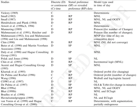
[image:7.544.44.500.114.473.2]

149 Both MNL and NL are special cases of the GEV model. The OGEV model allows for a 150 correlation parameter, for a pair of alternatives, which depends on the distance between the al-151 ternatives along some natural ordering, such as the clock time in time of day choice. The highest 152 correlation is expected to be found for adjacent alternatives. Alternatives at great distance from 153 each other will be independent as in the common MNL. In practice the number of free parameters

Table 1

Model types used in time of day studies

Studies Discrete (D)

or continuous (C) time

Stated preference (SP) or revealed preference (RP) data

Model type used in time of day

Vickrey (1969) C – Deterministic

Small (1982) D RP MNL

Small (1987) D RP MNL, NL and OGEV

Hendrickson and Plank (1984) D RP MNL

Arnott et al. (1990a,b, 1994) C – Deterministic

Mannering (1989) D RP Poisson (for number of Changes)

Mahmassani et al. (1991), Hatcher and Mahmassani (1992), Jou and Mahmassani (1994) and Liu and Mahmassani (1998)

D RP Poisson (for number of changes);

MNP (for time of day on consecutive days)

Chin (1990) D RP MNL (NL did not converge)

Bates et al. (1990) and Martin Voorhees Associates (1990)

D SP MNL

Daly et al. (1990) and Hague Consulting Group (1991)

D SP MNL

Polak and Jones (1994) D SP NL

Chin et al. (1995) D RP Incremental logit (MNL)

Accent and Hague Consulting Group (1995)

D SP MNL

Khattak et al. (1995) D SP Ordered probit (for changing)

De Palma and Rochat (1996) C RP Ordered probit (number of changes)

Wang (1996) C RP Weibull and log-logistic hazard

COWI et al. (1997) D SP NL

De Palma et al. (1997) D SP OLS & Tobit (for change in minutes)

Bhat (1998a) D RP MNL, NL and OGEV

Bhat (1998b) D RP MNL and EClogit

Bradley et al. (1998) D RP NL

Havnetunnelgruppen (1999) D SP NL and EClogit

van Vuren et al. (1999) and Hague Consulting Group et al. (2000)

C RP Deterministic, with segmentation;

partially endogenous

(8)

UNCORR

ECTED

PROO

F

154 needs to be reduced to allow maximum likelihood estimation (with non-standard software). The 155 simplest OGEV arises when all correlation parameters are equal and apply only to adjacent pairs 156 of alternatives. When Bhat (1998a) estimated a model with MNL for mode choice and OGEV for 157 time of day choice with two different correlation parameters (one more than in NL) he found that 158 the MNL–OGEV performed significantly better than the MNL and the NL model. He concluded 159 that the latter two specifications lead to biased level-of-service estimates and inappropriate 160 evaluations of policy measures.

161 An even more general model than OGEV was presented by Koppelman and Wen (1999): the 162 paired combinatorial logit (PCL) model. This model allows for a different correlation between 163 each pair of alternatives. This correlation does not depend on the distance between the alterna-164 tives as in OGEV. This could be a useful step forward for modelling time of day because not only 165 can we assume that time periods that follow shortly after other time periods will be correlated, but 166 also similar but faraway periods (e.g. busiest hour of morning and evening peak) could be highly 167 correlated. The OGEV is a special case of the PCL. Koppelman and Wen also use the PCL in 168 estimation (non-standard software), though not on time of day choice but mode choice.

169 PCL has limits, but there are further more general models, even within the GEV family (Daly, 170 2001). An even more general discrete choice model is the multinomial probit (MNP) which could 171 involve estimating a complete variance–covariance matrix for all alternatives. The major disad-172 vantage of MNP is that with many alternatives (meaning 3 or more), estimation is very cum-173 bersome due to the multiple integrals in the likelihood function. Therefore researchers have been 174 investigating the possibilities––with some success––of simulating the likelihood function or the 175 moments of the distribution by drawing from statistical distributions (e.g. Bolduc, 1999). Also the 176 number of free parameters in the variance–covariance matrix in most empirical work is reduced 177 considerably. Liu and Mahmassani (1998) used MNP for their time of day and route choice model 178 for consecutive days, without applying such simulation methods, but they have access to a Cray 179 supercomputer.

180 The EClogit or mixed MNL model has been known for some time (Cardell and Dunbar, 1980; 181 Ben-Akiva and Bolduc, 1991) and was put forward by several authors (e.g. McFadden and Train, 182 1997; Bhat, 1998b) in the late nineties as a highly flexible, yet practical, model type. It is no less 183 general than the MNP model in that it can also estimate a complete variance–covariance matrix. 184 Unlike MNP it can also handle asymmetric disturbances. EClogit can approximate the MNP; 185 MNP is the limiting case of EClogit. According to McFadden and Train (1997), EClogit can 186 approximate as closely as one pleases not only MNP but also any other discrete choice model 187 based on random utility maximisation, including OGEV and PCL. Therefore, although MNP, 188 OGEV and PCL are not special cases of EClogit, EClogit can serve as an approximation for these. 189 We therefore have chosen to use EClogit to model mode and time of day choice (also see Section 190 4).

191 The basic idea of any error components model is that it parameterises the variance–covariance 192 matrix, by adding components to the MNL model. The utility function in the MNL is:

Uk¼ X

r

(9)

UNCORR

ECTED

PROO

F

194 In which, Uk is the utility for decision-maker from alternative k; br is the parameter to be esti-195 mated forrth attribute; ek is the error term; follows extreme value type 1 distribution; xkr is the 196 measured attributer for alternative k.

197 In the EClogit model, the utility function becomes:

Uk ¼ X

r

b_rxkrþ X

s X

t

g_swk_stntþek ð3Þ

199 In Eq. (3) the following new components are added to MNL: n_t is the error component, dis-200 tributed fð0;1Þ, for which there can be several error components; g_s is the parameter to be es-201 timated;wk _{a general weighting matrix, based on data and/or fixed by the analyst, for alternative} 202 k, with rows s corresponding to the coefficients g and columns t corresponding to the error 203 componentsn.

204 If n and e follow the multivariate normal distribution, this model is MNP. In the EClogit 205 specification witheGumbel distributed however, the choice probabilitiesconditional on the error

206 componentstake the familiar MNL form. The unconditional choice probabilities are derived by 207 integration of the conditional MNL choice probabilities over the distribution of the error com-208 ponents. The latter distribution is usually evaluated using Monte Carlo simulation (drawing from 209 the distribution of n). The commonly used estimation method is called maximum simulated 210 likelihood. Different assumptions on the structure of the variance–covariance matrix for error 211 components can lead to different model specifications:

212 • _{MNL and NL are a special case of EClogit (NL by approximation).}

213 • _{The varying and random coefficients model can be written as EClogit models.}

214 • _{The model can be used for data sets with repeated measurements for the same individual (it is}

215 therefore an alternative to estimating thet-values using the Jack-knife method, providing we 216 know the structure of the interpersonal variation) by including individual-specific components; 217 the same specification can be used for panel data.

218 • _{It can approximate all other known discrete choice random utility models (e.g. MNP, OGEV}

219 and PCL).

220 3. The stated preference survey

221 The population from which respondents were recruited consists of persons travelling in the 222 extended peak periods (6.00–11.00 and 15.00–19.00 h during working days) as car drivers or train 223 passengers within The Netherlands. Respondents were recruited for participation in the actual 224 stated preference survey from an existing panel or from short recruitment interviews at train 225 stations and at a petrol station beside a motorway. The estimation sample contains information 226 on more than 1000 travellers.

(10)

UNCORR

ECTED

PROO

F

231 within a pre-specified mode and purpose combination. This information was used to customise 232 the stated preference experiments.

233 Three different stated preference questionnaires were developed:

234 (1) a questionnaire for home-based (HB) tours by car drivers (travel purposes can be home to 235 work, HB business or other, including education);

236 (2) a questionnaire for non-home-based (NHB) business trips by car drivers; and

237 (3) a questionnaire for HB tours by train travellers (purposes can be home to work, business, ed-238 ucation and other).

239 The stated preference questionnaires for car drivers (both the one for tours and the one for 240 trips) contain two choice experiments:

241 (1) a first experiment without road pricing focussing on the trade-off between departure time and 242 travel time (especially influenced by congestion); and

243 (2) a second experiment with peak pricing.

244 For the interviews with train passengers, a similar two-experiment structure was set up:

245 (1) the first experiment deals with choices using the present fare system; and

246 (2) the second experiment includes extra peak charges (also taking into account that there are re-247 duced fares for travel after 9.00 AM already).

248 In each of the stated preference experiments three or four alternatives were presented on the 249 same screen:

250 • _{The first alternative contains departure time options close to the observed departure times (the}

251 same or a little earlier/later).

252 • _{The second alternative contains departure times which are considerably earlier (in the road}

253 pricing experiments all travel in the morning takes place before the morning peak charging pe-254 riod; the car trips in the afternoon might coincide with the afternoon peak charges; in the train 255 peak charging experiments the travel takes place before the peak charging period, which refers 256 to the morning peak only).

257 • _{The third alternative contains departure times that are considerably later, to travel after the end}

258 of the morning peak charging (using the same rules as mentioned above for earlier departure 259 times).

260 • _{The fourth alternative refers to another mode than that observed (public transport for car}

trav-261 ellers and car for train travellers) and is presented only to travellers who state they could use the 262 alternative mode.

263 The attributes presented for these alternatives include:

(11)

UNCORR

ECTED

PROO

F

266 (3) departure time from destination;

267 (4) arrival time at home; 268 (5) tour travel time;

269 (6) duration of stay at destination;

270 (7) travel cost not including (extra) peak charge; 271 (8) peak charge (second experiment only); 272 (9) probability of a seat (train only); and 273 (10) frequency (train only).

274 The stated preference survey contains both relatively small (10–20 min) shifts in departure time 275 and large shifts (1 h or more).

276 By presenting the experiments this way, we have included the options that a respondent has in 277 reality (and thereby made the experiment look as much as possible like ÔrealityÕ) when facing 278 (severe) congestion or peak pricing: staying with the chosen mode at or close to the chosen de-279 parture times, travelling earlier, travelling later and changing mode (stop making this tour can 280 also be chosen). Furthermore, by presenting an alternative which is the same as the observed 281 situation, or close to it on each screen, the respondent is reminded of the present circumstances 282 with all the information on preferences and constraints that it contains, so that the choice will be 283 Ôtied to realityÕ. The number of screens per experiment is fixed at eight (giving eight choice ob-284 servations for the experiment without peak pricing and eight for the experiment with peak pricing 285 per respondent, all 16 screens with up to four alternatives per screen).

286 The four-alternatives-on-a-screen presentation departs from the standard presentation in 287 transport applications of stated preference with binary choices. Comparing four alternatives at the 288 same time is more difficult for the respondents, but recent experiments have shown that re-289 spondents are capable of giving consistent and plausible answers to complicated choice tasks 290 (Louviere and Hensher, 2000). In the pilot we tested whether respondents can cope with this task 291 of a four alternative comparison, and concluded that this was the case.

292 4. Estimation results

293 4.1. Model specification and estimation method

(12)

UNCORR

ECTED

PROO

F

303 (1) simultaneous models for time of day choice for both tour legs; and

304 (2) simultaneous models for time of day choice for the outward trip and activity duration, with 305 penalties for shorter or longer than preferred activity duration (following Polak and Jones, 306 1994).

307 Polak and Jones (1994) also used the tour concept for time-of-day choice instead of the 308 commonly used trip concept. In their paper they establish a link between the timing decision for 309 both legs of the tour and the activity scheduling, in which Ô. . . the timing of travel follows as a 310 consequence of the interplay between time varying patterns of destination utility and travel cost_Õ. 311 This concept was implemented in the APRIL (assessment of pricing of roads in London) model to 312 assess road pricing schemes in London.

313 These specifications did not lead to completely identical model results, presumably because of 314 slight inconsistencies in preferences for activity duration and arrival time at home. The second 315 category of models performed best for all four travel purposes, and was used in the models 316 presented below. The utility functions of the estimated models are based on the Vickrey–Small 317 utility functions (Eq. (1)), with scheduling penalty terms measured in minutes.

318 For a person observed making a car tour for some travel purpose, the utilityfunctions con-319 sidered in the estimations include:

U0¼aCARTIME0þboEARLY0þcoLATE0þbrREARLY0þcrRLATE0þdCARCOST0þ

U1¼aCARTIME1þboEARLY1þbrREARLY1þdCARCOST1þg1TIMDIF1n1þ

U2¼aCARTIME2þcoLATE2þcrRLATE2þdCARCOST2þg2TIMDIF2n2þ

U3¼aPTTIME3þboEARLY3þcoLATE3þbrREARLY3þcrRLATE3 þdPTCOST3þg3n3þ

ð4Þ

321 Many more variables (especially socio-economic attributes) have in practice been included, but 322 are not shown in this example to simplify the presentation. All utility functions include error terms 323 that follow the extreme value type I distribution.

324 The subscripts 0, 1, 2, 3 refer to the four alternatives presented on a screen in the stated 325 preference survey:

326 (1) observed mode and time of day; 327 (2) observed mode, considerably earlier; 328 (3) observed mode, considerably later; and 329 (4) different mode, observed time of day.

(13)

UNCORR

ECTED

PROO

F

337 LATE is the late schedule penalty for the outward leg: the difference in minutes between the 338 presented departure time and the preferred departure time, if presented departure time is after the 339 preferred departure time; otherwise zero; REARLY is the early schedule penalty for the return 340 leg: the difference in minutes between the preferred departure time and the presented departure 341 time, if presented departure time is before the preferred departure time; otherwise zero; RLATE is 342 the late schedule penalty for the return leg: the difference in minutes between the presented de-343 parture time and the preferred departure time, if presented departure time is after the preferred 344 departure time; otherwise zero;g1, g2 and g3 are the coefficients for the error components to be

345 estimated; TIMEDIF1 and TIMEDIF2 are the difference between presented time of day and

346 observed time of day in minutes; n1, n2 and n3 are error components drawn from a standard

347 normal distribution.

348 For a person observed making a tour by train the utility functions (again for the four alter-349 natives presented on a screen) could for example be:

U4¼aPTTIME4þboEARLY4þcoLATE4þbrREARLY4þcrRLATE4þdPTCOST4þ

U5¼aPTTIME5þboEARLY5þbrREARLY5þdPTCOST5þg1TIMDIF5n1þ

U6¼aPTTIME6þcoLATE6þcrRLATE6þdPTCOST6þg2TIMDIF6n2þ

U7¼aCARTIME7þboEARLY7þcoLATE7þbrREARLY7þcrRLATE7

þdCARCOST7þg3n3þ

ð5Þ

351 Finally for a person observed making a car trip (only for NHB business travel), the utility 352 functions are:

U8 ¼aCARTIME8þboEARLY8þcoLATE8þdCARCOST8þ

U9 ¼aCARTIME9þboEARLY9þdCARCOST9þg1TIMDIF9n1þ

U10¼aCARTIME10þcoLATE10þdCARCOST10þg2TIMDIF10n2þ

U11¼aPTTIME11þboEARLY11þcoLATE11þdPTCOST0þg3n3þ

ð6Þ

354 Here, CARTIME, CARCOST, PTTIME and PTCOST refer to a trip, not a tour.

355 Some respondents have a choice between three alternatives, because the alternative mode was 356 not available (e.g. if no public transport available, or train users without a driving licence). Be-357 cause we condition on car availability, we did not include a car availability measure, such as the 358 cars to licences ratio, in the utility functions.

359 Thevalue of time (VOT) is defined asa=d. This gives the VOT in guilders/minute. After mul-360 tiplying by 60 we obtain the VOT in guilders/hour. Furthermore we shall calculatetrade-off ratios

361 for the scheduling penalties versus the travel time coefficients:

362 (1) being early on outward leg (bo=a); 363 (2) being early on return leg (br=a); 364 (3) being late on outward leg (co₌_a_{); and}

(14)

UNCORR

ECTED

PROO

F

366 These ratios give the importance of being 1 min early or late in terms of a minute travel time. If 367 these ratios are between zero and one, a minute scheduling delay is not as bad as a minute travel 368 time.

369 The error components that were tested (the first three are represented in the above equations) are:

370 • _{A component that is proportional to the shift in departure time in the considerably earlier}

al-371 ternative (U1, U5,U9, using the notation as in the utility functions in Eqs. (4)–(6)); the greater

372 the shift, the lower the correlation between alternatives should be.

373 • _{A component that is proportional to the shift in departure time in the considerably later}

alter-374 native (U2,U6,U10); the greater the shift, the lower the correlation between alternatives should

375 be.

376 • _{A component for mode shift (U}₃_,_U₇_,_U₁₁_{); to test the hypothesis that shifting time is easier than}

377 shifting mode.

378 • _{A component that is proportional to the change in cost in the considerably earlier alternative}

379 (U1, U5, U9); the greater the shift, the lower the correlation between alternatives should be.

380 • _{A component that is proportional to the change in cost in the considerably later alternative (U}₂_,

381 U6, U10); the greater the shift, the lower the correlation between alternatives should be.

382 • _{A component that is proportional to the change in travel time in the considerably earlier}

alter-383 native (U1, U5,U9); the greater the shift, the lower the correlation between alternatives should

384 be.

385 • _{A component that is proportional to the change in travel time in the considerably later}

alterna-386 tive(U2,U6,U10); the greater the shift, the lower the correlation between alternatives should be.

387 Below is a selection of the best time of day models obtained for each of the four purposes. 388 Results are presented for models with Jack-knife 2and without (calledÔoriginal modelÕ) Jack-knife 389 estimation. The Jack-knife (see Cirillo et al., 2000) was used here to correct for the repeated 390 measurements bias, which leads to overstated t-ratios and may correct for other specification 391 errors as well. Future work may include using error components for this as well and comparing 392 the outcomes with those of the Jack-knife. The models were estimated using the discrete choice 393 model estimation software ALOGIT4. The error components are simulated from the normal 394 distribution using 1000 pseudo-random draws.

395 4.2. Estimation results for commuting

396 The estimation results for commuting are in Table 2. After the Jack-knife estimation, all the 397 estimated coefficients have the expected sign and are significant at the 95% confidence level, except 398 for the dummy for working at home regularly and one of the car cost coefficients. The latter 399 coefficient is significant at 90%. Younger persons, part-time workers and persons with a lower 400 education level have a lower likelihood of shifting to earlier or later periods. Single workers 401 travelling by train have an increased flexibility with regards to time of day choice.

2

(15)

UNCORR

ECTED

[image:15.544.41.498.111.638.2]

PROO

F

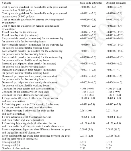
Table 2

Estimation results for commuting (t-ratios in brackets)

Variable Jack-knife estimates Original estimates

Cost by car (in guilders) for households with gross annual income below 60,000 guilders

)0.0130 ()1.7) )0.0143 ()7.5)

Cost by car (in guilders) for households with gross annual income above 60,000 guilders

)0.0111 ()2.6) )0.0100 ()5.8)

Cost by train (in guilders) for persons not compensated by employer

)0.0429 ()2.8) )0.0375 ()5.4)

Cost by train (in guilders) for persons compensated by employer

)0.0142 ()2.2) )0.0132 ()5.4)

Travel time by car (in minutes) )0.0141 ()5.2) )0.0139 ()13.2) Travel time by train (in minutes) )0.0162 ()3.6) )0.0155 ()12.7) Early schedule penalty (in minutes) for the outward leg

for persons with flexible working hours

)0.0153 ()5.7) )0.0159 ()14.9)

Early schedule penalty (in minutes) for the outward leg for persons without flexible working hours

)0.0166 ()5.9) )0.0172 ()14.2)

Late schedule penalty (in minutes) for the outward leg for persons with flexible working hours

)0.0191()3.3) )0.0210 ()15.6)

Late schedule penalty (in minutes) for the outward leg for persons without flexible working hours

)0.0290 ()6.6) )0.0304 ()15.7)

Increased participation time penalty (in minutes) for persons with flexible working hours

)0.0098 ()4.7) )0.0096 ()6.5)

Increased participation time penalty (in minutes) for persons without flexible working hours

)0.0071 ()2.6) )0.0074()4.7)

Decreased participation time penalty (in minutes) for persons with flexible working hours

)0.0041 ()4.2) )0.0038 ()3.6)

Decreased participation time penalty (in minutes) for persons without flexible working hours

)0.0055 ()4.0) )0.0063 ()4.5)

Constant for train earlier and later alternatives )1.05 ()6.6) )1.06 ()10.2) Constant for car alternative for train users )1.63 ()3.3) )1.64 ()9.9) Constant for train alternative for car users )1.15 ()2.5) )1.30 ()10.9) 1 if age under 40 years, 0 otherwise; for car earlier

and later alternatives

)0.510 ()5.8) )0.498 ()9.5)

1 if working part time (<32 h a week), 0 otherwise; for car and train earlier and later alternatives

)0.471 ()2.8) )0.447 ()5.3)

1 if single worker; 0 otherwise; for train earlier and later alternatives

0.761 (3.0) 0.771 (4.2)

1 if low education level; 0 otherwise; for car and train earlier and later alternatives

)0.895 ()5.5) )0.886 ()10.0)

1 if working home regularly; 0 otherwise; for car and train earlier and later and switch mode alternatives

)0.158 ()0.8) )0.139 ()1.9)

Error component: departure time difference between the peak and the earlier retimed alternative

0.0093 (5.0) 0.0089 (11.2)

Error component: departure time difference between the peak and the later retimed alternative

0.0117 (2.8) 0.0123 (10.1)

Rho-squared (0) 0.333 0.333

Rho-squared (c) 0.096 0.096

(16)

UNCORR

ECTED

PROO

F

402 To judge the estimation results for travel time, cost and delay, one can have a look at the values 403 of time and other trade-off ratios (see Section 4.1). In Table 3 are a number of trade-off ratios 404 derived from the commuting model in Table 2.

405 The values of time are clearly higher than the values used in The Netherlands for project 406 evaluation (about 17 guilders/h). 3This has been found for some other time of day models as well 407 and is also found for the other purposes in this study (except business). It appears that cost 408 differences are not as strong in persuading travellers to shift time as are time differences, perhaps 409 because the time differences already imply a change to activity schedules.

[image:16.544.52.504.112.436.2]

410 The scheduling trade-off ratio of 1.08 for car drivers with flexible working hours being early 411 (Jack-knife estimation) in Table 3 is the result of dividing the coefficient₎0.0153 from Table 2 by 412 the car travel time coefficient₎0.0141 (but at higher precision). This result implies that 1 min too 413 early is valued to be slightly worse than 1 min of travel time. Most of the ratios of the schedule 414 delay penalty coefficients, both for too early and too late, to travel time are between 1 and 1.5; half 415 an hour earlier or later at work gives the same disutility as 30–45 min travel time. In the previous

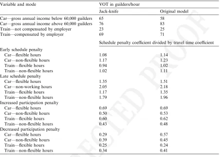
Table 3

Trade-off ratios for commuting

Variable and mode VOT in guilders/hour

Jack-knife Original model

Car––gross annual income below 60,000 guilders 65 58 Car––gross annual income above 60,000 guilders 76 83

Train––not compensated by employer 23 25

Train––compensated by employer 69 71

Schedule penalty coefficient divided by travel time coefficient

Early schedule penalty

Car––flexible hours 1.08 1.14

Car––non-flexible hours 1.17 1.23

Train––flexible hours 0.94 1.02

Train––non-flexible hours 1.02 1.11

Late schedule penalty

Car––non-working hours 2.05 2.18

Increased participation penalty

Decreased participation penalty

3

(17)

UNCORR

ECTED

PROO

F

416 1989 time of day stated preference survey in The Netherlands, these ratios were generally between 417 0.5 and 1 for commuting. Time of day shifting appears to be less sensitive now, perhaps because 418 many travellers have already shifted to less preferred time of day periods in response to increasing 419 congestion. The disutility from arriving early is now very similar to that of being late. The above 420 discussion referred to the outward leg. For the participation time decision, working too long or 421 too short is generally preferred to an equivalent amount of travel time.

422 The error components used in the best model for commuting are:

423 (1) a component that is proportional to the shift in departure time in the considerably earlier al-424 ternative: the greater the shift, the lower the correlation between alternatives will be; and 425 (2) a component that is proportional to the shift in departure time in the considerably later

alter-426 native the greater the shift, the lower the correlation between alternatives will be.

427 For both error components, the closer the coefficient is to zero, the higher the degree of sub-428 stitution. The sign of the error components is of no importance, but we would expect about the 429 same absolute size for both departure time shift error components. This is indeed what we find in 430 estimation. Error components proportional to the cost and travel time differences were tried as 431 well but did not significantly improve the models; nor did an error component for mode shift for 432 commuting. This finding implies that––all else equal––these models imply a greater elasticity for 433 mode shifting than for time shifting.

434 4.3. Estimation results for business travel

435 The estimation results for HB business tours and NHB business trips are in Table 4.

436 In the Jack-knife estimates of the business model, the coefficients for the early and late schedule 437 penalties for train are only significant at the 90% confidence level. Two participation time coef-438 ficients, the education dummy and one of the intercept terms are not significant at the 90% level. 439 The other coefficients are significant at 95% and have the expected signs. Again younger persons 440 are less likely to shift to off-peak. The trade-off ratios are in Table 5.

441 To calculate the VOT in these models, which used the log cost formulation, the ratio of the time 442 coefficient to the log cost coefficient is divided by the average time travelled. This gives an ap-443 proximate average VOT––in fact according to the model the VOT varies substantially among the 444 travelling population, proportionately to the journey cost.

445 The values of time are somewhat higher than the officially recommended values (almost 55 446 guilders, but also including the valuation by the employer). Again, several of the outward leg 447 scheduling penalty coefficients exceed the travel time coefficients, whereas for participation time, 448 the penalty coefficients are lower than those for travel time.

449 4.4. Estimation results for education tours

(18)

UNCORR

ECTED

PROO

F

Table 5

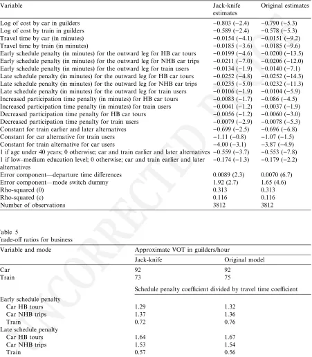
Trade-off ratios for business

Variable and mode Approximate VOT in guilders/hour

Car 92 92

Train 73 75

Car HB tours 1.29 1.32

Car NHB trips 1.37 1.36

Train 0.72 0.76

Car HB tours 1.64 1.67

Car NHB trips 1.53 1.54

Train 0.57 0.56

Increased participation penalty––car HB tours 0.54 0.57

[image:18.544.52.503.113.629.2]

Decreased participation penalty––train 0.43 0.42

Table 4

Estimation results for business (t-ratios in brackets)

Variable Jack-knife

estimates

Original estimates

Log of cost by car in guilders )0.803 ()2.4) )0.790 ()5.3) Log of cost by train in guilders )0.589 ()2.4) )0.578 ()5.3) Travel time by car (in minutes) )0.0154 ()4.1) )0.0151 ()9.2) Travel time by train (in minutes) )0.0185 ()3.6) )0.0185 ()9.6) Early schedule penalty (in minutes) for the outward leg for HB car tours )0.0199 ()4.6) )0.0200 ()13.5) Early schedule penalty (in minutes) for the outward leg for NHB car trips )0.0211 ()7.0) )0.0206 ()12.0) Early schedule penalty (in minutes) for the outward leg for train users )0.0134 ()1.9) )0.0140 ()7.1) Late schedule penalty (in minutes) for the outward leg for HB car tours )0.0252 ()4.8) )0.0252 ()14.3) Late schedule penalty (in minutes) for the outward leg for NHB car trips )0.0235 ()5.0) )0.0232 ()11.3) Late schedule penalty (in minutes) for the outward leg for train users )0.0106 ()1.9) )0.0104 ()5.9) Increased participation time penalty (in minutes) for HB car tours )0.0083 ()1.7) )0.086 ()4.5) Increased participation time penalty (in minutes) for train users )0.0041 ()1.2) )0.0037 ()1.9) Decreased participation time penalty for HB car tours )0.0056 ()1.2) )0.0060 ()3.0) Decreased participation time penalty for train users )0.0079 ()2.9) )0.0078 ()5.3) Constant for train earlier and later alternatives )0.699 ()2.5) )0.696 ()6.8) Constant for car alternative for train users )1.11 ()0.8) )1.07 ()1.5) Constant for train alternative for car users )4.00 ()3.1) )3.87 ()4.9) 1 if age under 40 years; 0 otherwise; car and train earlier and later alternatives )0.559 ()3.7) )0.553 ()7.8) 1 if low–medium education level; 0 otherwise; car and train earlier and later

alternatives

)0.174 ()1.3) )0.179 ()2.2)

Error component––departure time differences 0.0089 (2.3) 0.0070 (6.7)

Error component––mode switch dummy 1.92 (2.7) 1.65 (4.6)

Rho-squared (0) 0.313 0.313

(19)

UNCORR

ECTED

PROO

F

453 In the model presented for education, some of the scheduling variables were clearly not sig-454 nificant, even before Jack-knifing. These have been removed and the model has been re-estimated 455 without those variables. Persons with a low education level (going mostly to schools with fixed 456 school hours starting and ending in the peak periods) have a higher probability of selecting the 457 peak alternative.

458 The trade-off ratios for this travel purpose are in Table 7. The values of time for car are in line 459 with official recommendations, but those for train are particularly high. For education all 460 scheduling and participation penalty coefficients represent a lower disutility than travel time.

461 4.5. Estimation results for ‘other purposes’

462 Finally, the estimation results forÔother purposesÕare given in Table 8.

[image:19.544.42.505.112.300.2]

463 All the coefficients have the sign we expected and are significant at 95%, except for cost, two 464 alternative-specific constants and one of the participation time penalties for train. The departure

Table 6

Estimation results for education (t-ratios in brackets)

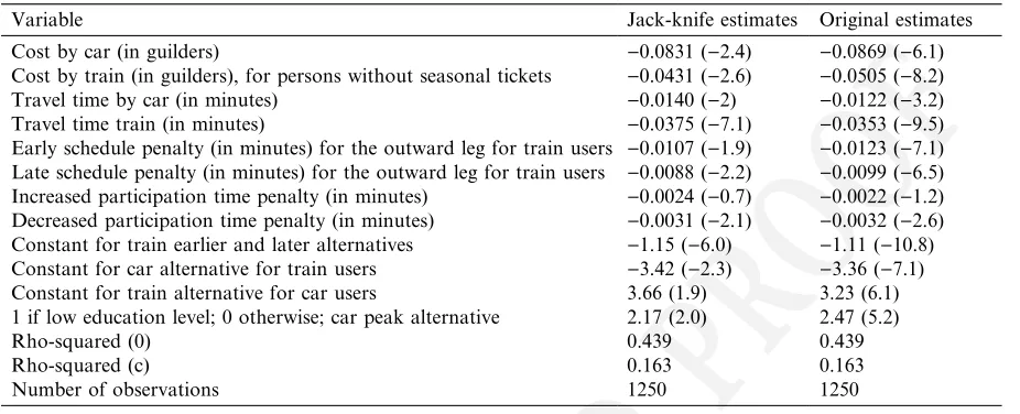
Variable Jack-knife estimates Original estimates

Cost by car (in guilders) )0.0831 ()2.4) )0.0869 ()6.1)

Cost by train (in guilders), for persons without seasonal tickets )0.0431 ()2.6) )0.0505 ()8.2) Travel time by car (in minutes) )0.0140 ()2) )0.0122 ()3.2) Travel time train (in minutes) )0.0375 ()7.1) )0.0353 ()9.5) Early schedule penalty (in minutes) for the outward leg for train users )0.0107 ()1.9) )0.0123 ()7.1) Late schedule penalty (in minutes) for the outward leg for train users )0.0088 ()2.2) )0.0099 ()6.5) Increased participation time penalty (in minutes) )0.0024 ()0.7) )0.0022 ()1.2) Decreased participation time penalty (in minutes) )0.0031 ()2.1) )0.0032 ()2.6) Constant for train earlier and later alternatives )1.15 ()6.0) )1.11 ()10.8) Constant for car alternative for train users )3.42 ()2.3) )3.36 ()7.1) Constant for train alternative for car users 3.66 (1.9) 3.23 (6.1) 1 if low education level; 0 otherwise; car peak alternative 2.17 (2.0) 2.47 (5.2)

Rho-squared (0) 0.439 0.439

Number of observations 1250 1250

Table 7

Trade-off ratios for education

Car 10 8

Train 52 42

Early schedule penalty––train 0.28 0.35

Late schedule penalty––train 0.23 0.28

Increased participation penalty––train 0.06 0.06

(20)

UNCORR

ECTED

PROO

F

465 time difference component coefficients have about the same size. A housewife has a lower prob-466 ability of being able to shift departure time (presumably because of time constraints at home). 467 Persons with a low education level have more difficulty in shifting departure time as well. 468 Trade-off values for other purposes are found in Table 9. The values of time are clearly higher 469 than the officially recommended values (about 11 guilders), but cannot be based on a significant 470 cost estimate. Three out of the four scheduling delay penalty coefficients exceed the travel time 471 coefficient and all the participation penalty coefficients are lower than the travel time coefficient.

472 4.6. Overview of estimation results

473 Many different specifications were tested for all four purposes, with the following results:

474 • _{EClogit generally outperformed MNL and NL, except for education tours.}

475 • _{A separate model for NHB business travel did not give acceptable coefficients (probably due to}

476 the limited number of observations); this was merged with HB business tours.

477 • _{For commuting, but not for all other purposes, quadratic scheduling penalties gave better}

re-478 sults than linear scheduling terms only (to get comparable values of time and other trade-off 479 values in the above tables we presented only linear models).

480 • _{For business travel, but not for the other purposes, logarithmic cost performed better than}

[image:20.544.48.504.113.385.2]

lin-481 ear cost.

Table 8

Estimation results for other purposes (t-ratios in brackets)

Variable Jack-knife

estimates

Original estimates

Cost (in guilders) )0.092 ()0.9) )0.0129 ()7.2)

Travel time by car (in minutes) )0.0157 ()2.6) )0.0156 ()11.2) Travel time by train (in minutes) )0.0170 ()4.4) )0.0179 ()12.4) Early schedule penalty (in minutes) for the outward leg for car users )0.0193 ()6.6) )0.0197 ()13.3) Early schedule penalty (in minutes) for the outward leg for train users )0.0121 ()3.1) )0.0094 ()5.5) Late schedule penalty (in minutes) for the outward leg for car users )0.0264 ()5.5) )0.0249 ()13.9) Late schedule penalty (in minutes) for the outward leg for train users )0.0174 ()2.9) )0.0124 ()5.2) Increased participation time penalty (in minutes) for car users )0.0056 ()3.1) )0.0059 ()4.0) Increased participation time penalty (in minutes) for train users )0.0077 ()3.3) )0.0090 ()5.5) Decreased participation time penalty (in minutes) for car users )0.0051 ()2.6) )0.0050()2.5) Decreased participation time penalty (in minutes) for train users )0.0057 ()1.6) )0.0056 ()3.2) Constant for train earlier and later alternatives )0.125 ()0.5) )0.265 ()2.7) Constant for car alternative for train users )0.689 ()1.2) )0.849 ()3.8) Constant for train alternative for car users )1.78 ()4.3) )1.76 ()10.6) 1 if housewife; 0 otherwise; car and train earlier and late alternatives )0.340 ()3.4) )0.342 ()4.2) 1 if low education level; 0 otherwise; car earlier and switch mode alternatives )0.624 ()3.5) )0.639 ()6.9) Error component: departure time difference, earlier alternative 0.0100 (6.0) 0.0104 (10.2) Error component: departure time difference, later alternative 0.0178 (3.3) 0.0107 (4.4)

Rho-squared (0) 0.262 0.262

(21)

UNCORR

ECTED

PROO

F

482 • _{Splitting the cost coefficients by income group did not produce satisfactory results, except for}

483 commuting tours.

484 • _{A cost of zero for holders of seasonal passes worked best for education and other purposes, not}

485 for commuting tours and business travel.

486 • _{For train commuters, cost coefficients that differentiate between employees receiving}

compen-487 sation and employees not receiving compensation gave plausible values and a significant im-488 provement in likelihood. Delay coefficients that differentiate between employees with and 489 without flexible work hours did the same for commuters by train and car.

490 5. Simulation results

[image:21.544.43.519.114.332.2]

491 To get a good impression of the substitution patterns in the models estimated (nearby versus 492 faraway periods, mode versus time of day alternatives), we carried out several simulation runs for 493 car and train commuters. Fig. 1 shows the effect of an increase in the AM peak travel time 494 (between 7:00 and 9:00) on the outward leg departure time (Ôout changeÕ in the graph), on the 495 return leg departure time (Ôback changeÕ) and on mode switching for commuters initially travelling 496 by car. For the other purposes, the results were mostly rather similar to those for commuting. On 497 the vertical axis are the percentage changes in the number of trips (car trips in Fig. 1 and train 498 trips in Fig. 2), using the estimation sample. The horizontal axis gives the distribution over the 499 time of day alternatives (aggregated to 11 time slices) during an entire 24-h day and the alternative 500 to switch mode. Note that only the points in the graph indicate a value, the lines are drawn to 501 improve readability.

Table 9

Trade-off ratios for other purposes

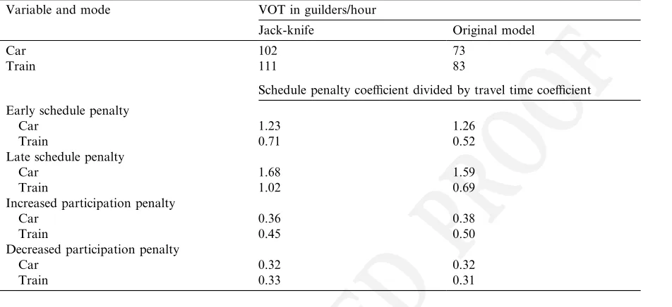
Car 102 73

Train 111 83

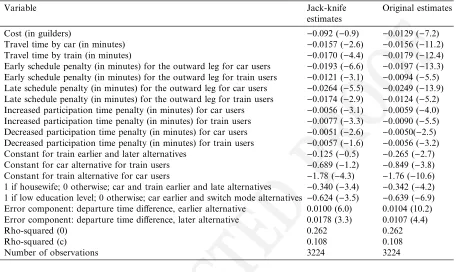
Car 1.23 1.26

Train 0.71 0.52

Car 1.68 1.59

Train 1.02 0.69

Increased participation penalty

Car 0.36 0.38

Train 0.45 0.50

Decreased participation penalty

Car 0.32 0.32

(22)

UNCORR

ECTED

PROO

F

502 Fig. 1 indicates that if the morning peak travel time increases, many commuters will change 503 their departure time for the outward leg. Instead of departing in the affected periods (7:00–9:00) 504 many will now depart during a neighbouring period, both of which increase by more than 4%. 505 One can also notice that quite a few make major shifts in outbound leg to 10:00–15:00 or 24:00– 506 6:00. As one could expect, this change has no impact on the travellers departing during the af-507 ternoon and the evening (15:00–24:00).

508 The effect on the return leg departure time is less important than on the outward leg, fewer 509 travellers are switching period. We can notice interesting changes in profiles both out and return, 510 e.g. small increases in returns between 6:00 and 7:00 and between 9:00 and 10:00 are presumably 511 people returning home in AM peak, while increases in returns between 15:00 and 16:00 and be-512 tween 19:00 and 24:00 are people affected on their outbound leg.

513 Some car commuters will also shift to the train. The number of train trips increases by 4%. 514 Given the small initial number of choices for train in the data base for this purpose, not as many

Fig. 1. Changes in time of day and mode choice (AM peak travel timeþ10%), car commuters only.

(23)

UNCORR

ECTED

PROO

F

515 go to the train as to neighbouring periods (of course this is also affected by the fact that the train is 516 also slowing down in the simulation).

517 Fig. 2 is similar to the previous one but deals with travellers initially using the train. Here the 518 car is much more important as an alternative relative to time shifts. One could assume that train 519 users are more scheduling-time constrained than car users and it is easier for them to change mode 520 than departure time. Also we should keep in mind when comparing the above two figures that 521 only for a limited number of trips where car (if available) is a good alternative there are good train 522 connections.

523 Shifts to neighbouring periods are even larger than on the previous chart for the outward leg as 524 well as for the return leg. No train users return in AM peak (night workers use cars), so all return 525 shifts are consequent on outward effect. One can note how these are earlier than for car users. 526 Many of those who change their choices switch to cars.

527 6. Conclusions and recommendations

528 A new stated preference survey into the time of day choice of travellers by car and train has 529 been carried out in The Netherlands. In this paper, these data have been used to estimate error 530 components models of time of day and mode choice.

531 In our estimation results, EClogit generally outperformed MNL and NL, except for education 532 tours. In the estimated models, for commuting, business and other purposes, arriving 30 min too 533 late or too early at the destination is valued to be worse than 30 min of travel time. For education 534 tours, the opposite is found. Longer than preferred activity participation time is generally valued 535 to be less important than an equivalent amount of travel time.

536 Simulation results with the estimated models show that for most purposes, the closer the two 537 time of day periods are in clock time, the greater will be the degree of substitution. If travel time or 538 cost in the peak increases, most travellers will shift to periods just before or after the peak. Many 539 train travellers will also shift to the car (more than will shift from car to train).

540 The new results indicate that time of day choice in The Netherlands is sensitive to changes in 541 peak travel time and cost and that policies that increase these peak attributes will lead to peak 542 spreading. However, the time of day sensitivities to travel time and cost changes in the (selective) 543 sample, in general seem to be lower than 10 years ago. 4

544 In this paper we applied the Jack-knife method to estimate coefficient values and standard 545 errors that do not suffer from the repeated measurements problem (multiple observations from the

4

(24)

UNCORR

ECTED

PROO

F

546 same individual, taken to be independent) of the stated preference data. An alternative method 547 would be to include individual-specific components, as are sometimes used in panel data models, 548 in the error components model. Further research is needed to compare these two ways of solving 549 the repeated measurement problem.

550 7. Uncited References

551 COWI et al. (1996), Daly (1999), Daly et al. (1998), Hague Consulting Group (1990), Kim and 552 Mannering (1992) and Polak et al. (1993).

553 References

554 Accent and Hague Consulting Group, 1995. The value of time on UK roads; Final report prepared for the Department

555 of Transport. Accent and HCG, London, The Hague.

556 Arnott, R., de Palma, A., Lindsey, R., 1990a. Departure time and route choice for the morning commute.

557 Transportation Research 24 (3), 209–228.

558 Arnott, R., de Palma, A., Lindsey, R., 1990b. Welfare effects of congestion tolls and heterogeneous commuters. Journal

559 of Transport Economics and Policy XXVIII-2, 139–161.

560 Bates, J.J., 1996. Time period choice modelling: a preliminary review. Final report for the Department of Transport––

561 HETA Division, John Bates Services.

562 Bates, J.J., Shepherd, N.R., Roberts, M., van der Hoorn, A.I.J., Pol, H.D.P., 1990. A model of departure time choice in

563 the presence of road pricing surcharges. In: PTRC 18th Summer Annual Meeting, Proceedings of Seminar H,

564 PTRC, London, pp. 215–226.

565 Ben-Akiva, M., Bolduc, M., 1991. Multinomial probit with autoregressive error structure. Cahier 9123, Department of

566 Economics, University Laval, Quebec.

567 Bhat, C., 1998a. Analysis of travel mode and departure time choice for urban shopping trips. Transportation Research

568 B 32 (6), 361–371.

569 Bhat, C., 1998b. Accomodating flexible substitution patterns in multi-dimensional choice modelling: formulation and

570 application to travel mode and departure time choice. Transportation Research B 32 (7), 455–466.

571 Bolduc, D., 1999. A practical technique to estimate multinomial probit models in transportation. Transportation

572 Research B 33, 63–79.

573 Bradley, M.A., Bowman, J.L., Shiftan, Y., Lawton K., Ben-Akiva, M.E., 1998. A system of activity-based models for

574 Portland, Oregon. Report prepared for the Federal Highway Administration Travel Model Improvement Program,

575 Washington, DC.

576 Cardell, N.S., Dunbar, F.C., 1980. Measuring the societal impact of automobile downsizing. Transportation Research

577 A 14 (5–6), 432–434.

578 COWI, Carl Bro, Hague Consulting Group, 1996. Updating of the Storebælt Traffic Model, Task 11––Analysis of

579 background time choice variables (passenger survey). CCH, Copenhagen.

580 COWI, Carl Bro, Hague Consulting Group, 1997. Updating of the Storebælt Traffic Model, Task 11––time choice

581 model results (passenger survey). CCH, Copenhagen.

582 Chin, A.T.H., 1990. Influences on commuter trip departure time decisions in Singapore. Transportation Research A 24

583 (5), 321–333.

584 Chin, K.K., van Vliet, D., van Vuren, T., 1995. An equilibrium incremental logit model of departure time and route

585 choice. In: PTRC 23rd European Transport Forum, Proceedings of Seminar F, PTRC, London. pp. 165–176.

586 Cirillo, C., Daly, A.J., Lindveld, K., 2000. Eliminating bias due to the repeated measurements problem. In: de Ortuuzar,

(25)

UNCORR

ECTED

PROO

F

588 Daly, A.J., 1999. The use of schedule-based assignments in public transport modelling. In: PTRC European Transport

589 Conference, Cambridge.

590 Daly, A.J., 2001. Recursive nested EV model. ITS Working Paper 559, University of Leeds.

591 Daly, A.J., Gunn, H.F., Hungerink, G.J., Kroes, E.P., Mijjer, P.H., 1990. Peak-period proportions in large-scale

592 modelling. In: PTRC 18th Summer Annual Meeting, Proceedings of Seminar H, PTRC, London. pp. 215–226.

593 Daly, A.J., Rohr, C., Jovicic, G., 1998. Application of models based on stated and revealed preference data for

594 forecasting passenger traffic between east and west Denmark. In: Meersman, H., van de Voorde, E., Winkelmans,

595 W. (Eds.), World Transport Research, Selected proceedings of the 8th World Conference on Transport Research,

596 vol. 3. Pergamon, Oxford.

597 De Palma, A., Rochat, D., 1996. Urban congestion and commuter behaviour: the departure time context. Revue

598 dÕEconomie Regionale et Urbaine 3, 467–488 (in French).

599 De Palma, A., Khattak, A.J., Gupta, D., 1997. CommutersÕ departure time decisions in Brussels. Transportation

600 Research Record, 1607.

601 Hague Consulting Group, 1990. De effecten van Rekening Rijden volgens het Landelijk Model, Rapport A: de

602 modelstructuur. HCG-rapport 027-2, Den Haag.

603 Hague Consulting Group, 1991. Stated Preference onderzoek: veranderingen in de vertrektijd onder invloed van

604 congestie. HCG-rapport 916, Den Haag.

605 Hague Consulting Group, Halcrow Fox, Imperial College, 1998. Modelling peak spreading and trip retiming––Phase

606 II––Assessment of current theory, operational models and assignment packages––Final version. Report for DETR

607 HETA, HCG-report 8013/2c, HCG-UK, Cambridge.

608 Hague Consulting Group, Halcrow Fox, Imperial College, 2000. Modelling peak spreading and trip retiming––Phase

609 II, Final Report. Report for DETR HETA, HCG-report 8013, HCG-UK, Cambridge.

610 Hatcher, S.G., Mahmassani, H.S., 1992. Daily variability of route and trip scheduling decisions for the evening

611 commute. TRB Annual Meeting.

612 Havnetunnelgruppen (Tetraplan, Hague Consulting Group, IFP-Trafikstudier), 1999. Copenhagen Eastern Harbour

613 Tunel project, passenger SP results. Havnetunnelgruppen, Kopenhagen.

614 Hendrickson, C., Plank, E., 1984. The flexibility of departure times for work trips. Transportation Research A 18 (1),

615 25–36.

616 Hyman, G., 1997. The development of operational models for time period choice. Department of the Environment,

617 Transport and the Regions, HETA Division, London.

618 Jou, R.C., Mahmassani, H.S., 1994. Day-to-day dynamics of commuter travel behaviour in an urban environment:

619 departure time and route decisions. In: 7th International Conference on Travel Behaviour, Valle Nevado, Chile.

620 Khattak, A.J., Schofer, J.L., Koppelman, F.S., 1995. Effect of traffic information on commutersÕpropensity to change

621 route and departure time. Journal of Advanced Transportation 29 (2), 193–212.

622 Kim, S.G., Mannering, F.L., 1992. Panel data and activity duration models: econometric alternatives and applications.

623 In: Conference on Panels in Transportation Planning, Lake Arrowhead, CA.

624 Koppelman, F.S., Wen, C.-H., 1999. The paired combinatorial logit model: properties, estimation and application.

625 Transportation Research B 34, 75–89.

626 Liu, Y.-H., Mahmassani, H.S., 1998. Dynamic aspects of commuter decisions under advanced traveler information

627 systems: modeling framework and experimental results. Transportation Research Record, 1645, Paper no. 98-0650,

628 pp. 111–119.

629 Louviere, J.J., Hensher, D.A., 2000. Combining sources of preference data. Resource paper for IATBR 2000, Gold

630 Coast Australia.

631 Mahmassani, H.S., Hatcher, S.G., Caplice, C.G., 1991. Daily variation of trip chaining, scheduling and path selection

632 behaviour of commuters. In: 4th IATB Conference, Quebec.

633 Mannering, F.L., 1989. Poisson analysis of commuter flexibility in changing routes and departure times. Transportation

634 Research B 23 (1), 53–60.

635 McFadden, D.L., 1981. Econometric models of probabilistic choice. In: Manski, C.F., McFadden, D.L. (Eds.),

636 Structural Analysis of Discrete Data, with Econometric Applications. The MIT Press, Cambridge, MA.

637 McFadden, D.L., 1978. Modelling the choice of residential location. In: Karlqvist, A. et al. (Eds.), Spatial Interaction

(26)

UNCORR

ECTED

PROO

F

639 McFadden, D.L., Train, K., 1997. Mixed MNL logit models for discrete responses. Working Paper, Department of

640 Economics, University of California at Berkeley.

641 The MVA Consultancy, 1990. Stated preference analysis for Rekening Rijden, final report prepared for the Projekteam

642 Rekening Rijden. The MVA Consultancy, Londen.

643 Paag, H., Daly, A.J., Rohr, C.L., 2000. Predicting use of the Copenhagen harbour tunnel. In: IATBR 2000, Gold

644 Coast, Australia.

645 Polak, J.W., Jones, P.M., 1994. A tour-based model of journey scheduling under road pricing. In: 73rd Annual Meeting

646 of the Transportation Research Board, Washington, DC.

647 Polak, J., Vythoulkas, P.C., Jones, P., Sheldon, R., Wofinden, D., 1993. TravellersÕchoice of time of travel under road

648 pricing. In: PTRC 21st Summer Annual Meeting, Proceedings of Seminar D (abstract only), PTRC, Londen.

649 Small, K.A., 1982. The scheduling of consumer activities: work trips. American Economic Review 72 (June), 467–479.

650 Small, K.A., 1987. A discrete choice model for ordered alternatives. Econometrica 55 (2), 409–424.

651 van Vuren, T., Carmichael, S., Polak, J., Hyman, G., Cross, S., 1999. Modelling peak spreading in continuous time. In:

652 PTRC European Transport Conference, Cambridge.

653 Vickrey, W.S., 1969. Congestion theory and transport investment. American Economic Review (Papers and

654 Proceedings) 59, 251–261.