Visualization notations, models and taxonomies

promoting access to White Rose research papers

White Rose Research Online

Universities of Leeds, Sheffield and York

http://eprints.whiterose.ac.uk/

White Rose Research Online URL for this paper:

http://eprints.whiterose.ac.uk/77898/

Paper:

Brodlie, KW and Mohd Noor, NF (2007)

Visualization notations, models and

taxonomies.

In: Lim, IS and Duce, D, (eds.) Theory and Practice of Computer

Graphics 2007, Eurographics UK Chapter Proceedings. Theory and Practice of

Computer Graphics 2007, 13-15 June 2007, University of Wales, Bath.

Visualization

Notations, Models and Taxonomies

Ken Brodlie and Nurul Mohd Noor

School of Computing, University of Leeds

Abstract

Visualization taxonomies are an important means of imposing some structure on a rather diverse field. We review some earlier work in this area, particularly work based on the use of a notation to label classes of visualization techniques that are appropriate to particular entities. We propose a new notation introducing it in the context of a new visualization reference model, one we hope will lead eventually to a means of describing visualizations in a clear and unambiguous way.

1. Introduction

There is a continuing interest in the development of taxonomies for visualization. A well-organised taxonomy can provide an important structuring of the field, grouping visualization techniques into classes according to some criteria. Moreover such a taxonomy can act as the basis for a much needed visualization ontology.

A good notation can help in the development of taxonomies, by providing a concise yet expressive description of the equivalence classes of visualization techniques. In this work-in-progress paper we chart the development of notations and taxonomies for visualization over the past twenty years, and relate this to work on reference models for visualization which provide an overall framework. We put forward a new reference model as an evolution of previous models, and suggest a new style of notation that may help develop a visualization taxonomy. Our long-term vision is an ability to describe visualizations in a clear and unambiguous manner, with a formal description that can be stored as metadata with a visualization for archival purposes.

2. Evolution of visualization taxonomies, notations, models and ontologies

One of the first proposals for a visualization taxonomy was put forward by Wehrend and Lewis (1990). They placed visualization problems and the associated techniques as the elements of a matrix whose rows are objects (such as scalars, directions, positions) and whose columns are operations (such as identify, locate, distinguish). Some 600 examples were classified by Wehrend in his MSc thesis according to this matrix scheme. Keller and Keller (1992) in their book “Visual Cues”, present a large variety of

visualization examples, each classified using Wehrend’s scheme. In addition, they distinguish the role of dependent and independent variables in the dataset to be visualized. However the classification is performed simply on examples, rather than being a systematic organisation of visualization techniques.

Brodlie (1992) takes the view that visualization is concerned with understanding the underlying field (or entity) from which a dataset has been sampled. Thus he aims to provide a taxonomy of entities expressed as a multivariate function of several independent variables. A notation, called the E-notation, is proposed, using a superscript to indicate the type of dependent variable and a subscript to indicate the type of dependent variable. Thus the superscript can take values S (scalar), V (vector), T (tensor), and the subscript is a number indicating the dimension – but using [] to indicate aggregation and {} to indicate an enumerated set. For example, a volumetric entity such as a temperature field in a cavity would be labelled as ES

3. This proved a useful means of classifying

techniques – that is, the notation acted as a label for equivalence classes of techniques which could be applied to visualize entities of that type. Thus the ES

3

notation acted as a label for volume visualization techniques such as isosurfacing and volume rendering, but did not attempt to distinguish between the two, quite different, approaches. Similar efforts were made in Brodlie (1993, 1994) and Gallop (1994), with further work by Wright (2005) in a new textbook on scientific visualization. While this approach does provide some structuring of techniques, and while Brodlie (1993) did try to label display techniques as well as entities, generally the approach lacks the ‘problem-oriented’ theme of Wehrend and Lewis, in which the user’s goal is incorporated into the classification process.

taxonomy with much broader scope, unifying the fields of scientific and information visualization. Their work is also notable for its underpinning by a reference model for visualization. In this model, they distinguish the data from the underlying object of study (similar to the entity in Brodlie, 1992), and show how visualizations are then derived on the basis of two models: the design model, in which the algorithm developer incorporates specific choices such as interpolation method, and the user model, in which the user selects the technique on the basis of their own mental model. Another important contribution is a clear definition of the datatypes involved in visualization, and we shall make use of this work later in this paper.

Work on reference models for visualization has proceeded in parallel to the efforts on taxonomies. A landmark contribution was the dataflow reference model proposed by Upson et al (1989) and Haber and McNabb (1990). This expressed the visualization process as a pipeline of elementary processes, each of type Filter (to refine the data), Map (to select a visualization idiom, turning numbers into geometrical representation) or Render (to display the geometry using computer graphics techniques). This model has served the community well: it acted as the basis for the development of Modular Visualization Environments (MVEs) in the late 1980s and early 1990s, and was extended to support collaborative visualization in the work of Wood et al (1997) and Duce et al (1998).

A different approach, first suggested by Duce, was proposed in Brodlie et al (2004). This saw visualization as a three layer process: a conceptual layer, in which a high level view of the required visualization is conceived; a logical layer, in which this view is refined in terms of specific pipelines of processes; and a physical layer, in which the pipeline is realised in terms of specific software and hardware resources. This can be seen in partnership with the Upson / Haber-McNabb model; and the conceptual layer has some affinity with the user model in the Tory – Moller work.

Ontologies provide a much broader structure to a subject than a simple classification or taxonomy. A visualization ontology will define the concepts involved in the subject and the relationship between them. A discussion of visualization ontologies is provided by Duke et al (2005). Work on notation and taxonomies can be a useful contribution to ontology research, and indeed Shu et al (2006) derive a visualization ontology starting from the E-notation mentioned earlier.

The work in this paper begins with a new look at reference models for visualization, since getting the framework correct is an important basis for subsequent work. This is covered in section 3. We then propose in section 4 a new notation – a development of the earlier E-notation. This is based on

the underlying entity, and therefore will correspond to the earlier taxonomies of Brodlie and Tory and Moller. Section 5 makes a brief mention of taxonomies and section 6 presents conclusions and the direction of our future work.

3. A Reference Model for Visualization

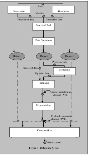
It is useful we believe to present any taxonomy in the context of a clear reference model. In this section we describe the model we are using; it is an evolution from the previous efforts described above. The model is shown in Figure 1. We distinguish data elements from processes that operate on data.

We start from the entity, or underlying field, we are trying to visualize. Our taxonomy will provide a notation to describe this in terms of its dependent and independent variables. The data to be visualized arises from a sampling by measurement of this field, or by a simulation process. We attach to this metadata

which will influence the visualization technique that is applied: for example, we might have metadata which specified that the underlying scalar field is everywhere positive, and so this can be incorporated in the interpolation process which recreates a model of the field for visualization.

The analytical task describes the goal of the user in carrying out the visualization. This is similar to the

operation of Wehrend and the user model of Tory and Moller. It is used to distinguish between different techniques that are applicable to a given entity. Essentially the description of the entity, the data, the metadata and the analytical task drive the route through the rest of the model – which itself is a variant on the Upson / Haber-McNabb model. The idea of including the analytical task is also motivated by the work of Tufte who has long argued that the design of a graphic must be driven by the mental task it is meant to support (see for example Zachary and Thralls, 2004).

The first process in the pipeline, Data Operations, applies necessary transformations to the data. This may include subsetting, or in the case of multivariate datasets, a splitting of the data into individual components. Thus the pipeline can fan out at this point.

Representation step, in which particular rendering attributes are added to create an RVE, or Realised Visualization Element. This separation of meaning from representation has its roots in the graphics standards work of the last century, when GKS for example, was defined in terms of a logical, workstation-independent, picture, and its subsequent representation on different workstations (see for example, Duce et al, 1983). Our thinking here is influenced also by Duce’s reference model for visualization, where the conceptual layer expresses a high level description of a visualization. Finally we

are also motivated by the potential use of the model for provenance and archiving of visualizations – we may wish to recreate the logical version exactly, but be unconcerned whether we reproduce the precise representation.

Finally we have a Composition step, in which the RVEs from the set of pipelines are combined in an appropriate way (often depending on the analytical task).

Observation

Data Operations

Modelling

Technique

Representation

Simulation

Abstract visualization element (AVE)

Realised visualization element (RVE) Observation data Simulation data

Processed data

Processed data

Equation data

Visualization Figure 1: Reference Model

Analytical Task

Dataset

1 Dataset2

DatasetN Entity

Metadata

4. Domino Notation

We now discuss a notation for describing the underlying field, or entity, that appears at the head of the reference model in Figure 1. We shall use the notation as a labelling for a visualization taxonomy.

We shall start from the earlier E-notation, but we shall aim to incorporate some of the improvements we can glean from the work of Tory and Moller, and others. Our guiding principles are:

• We wish to retain the separation into dependent and independent variables. • We wish to incorporate a better description

of datatypes.

• We wish to avoid redundancy in the notation (a criticism from Hopgood, c1993, of the E- notation was that the largest symbol, that is, E, is redundant!).

• We wish to find a distinctive and memorable idiom that will appeal to a wide community.

4.1 Datatypes for Dependent and Independent Variables

We shall simplify the earlier notation by using the same datatypes for dependent and independent variables – that is, the range and the domain. We shall consider four basic types: real (R); integer (Z) – with possibility of positive integers (Z+); and two categorical types, ordinal (O) where there is an ordering, and nominal (N) where there is not.

We see a need to distinguish the case where there is a single value, or a set of values – for example, an interval of real numbers rather than a single real number. We shall use the [] notation to indicate an interval. There is also increasing awareness in visualization that uncertainty may not just be expressed as a simple interval of values, but rather as a Probability Density Function (PDF) (see Love et al, 2005). At present we shall allow the [] notation to cover this case as well but it may be in the future that the two cases should be distinguished.

4.2 Dimensionality

We shall indicate the dimension of the independent variables as a multiplicative factor. Thus a three-dimensional volumetric domain would be designated RxRxR, or R3_{. This allows us also to have mixed type}

domains or ranges, for example, RxZ+_.

Multivariate data (i.e., type of dependent data) is indicated as an additive factor. Thus a CFD dataset of velocity, pressure and temperature would be designated as R3 _{+ R + R.}

4.3 Redundancy

To make the notation as compact as possible, we remove any symbol such as E that does not contribute identification information. Furthermore, we expect that in most instances we shall be dealing with a single value, rather than an interval or a PDF, and so we only include symbols (i.e. ‘[]’) if we wish to indicate an interval.

4.4 Metaphor

To make the notation memorable, we shall use a domino as the metaphor. The top indicates the dependent variable; the bottom the independent variable. Thus we have:

4.5 Simple Examples

A simple example is data representing values of a quantity measured at various points along an axis – for example, length of a bar measured at different temperatures and typically visualized as a 1-D graph. This would be represented as:

Another simple example but showing different datatypes is the following. Figure 2 shows a visualization of the range of temperature observed at Raleigh-Durham airport each day in December 1996. The entity here has a range that is an interval of real numbers, and a domain which is an ordinal variable – hence designated:

R

R

[R]

Figure 2 – Interval range and ordinal domain

4.6 A more complex visualization

The notation can also be used in more complex cases. For example, consider the situation where the visualization is of the population of the countries in the world. This would be an integer dependent variable, with a 2D ‘region’ independent variable, hence the notation:

However suppose the entity was the male-female split of population: then the dependent variable is another entity in itself, namely an integer dependent variable and a nominal independent variable (male, female). We can then nest the dominos as follows:

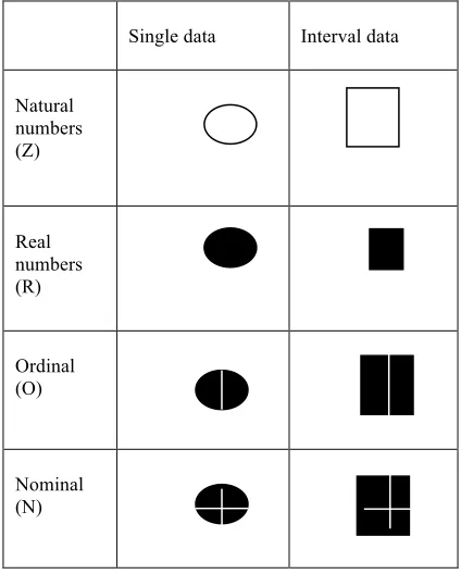
4.7 Another domino representation

We are also exploring different representations of the dominos. For example, rather than use letters as symbols, can we take the domino metaphor further and use dots. Here is a suggestion:

Single data Interval data

Natural numbers (Z)

Real numbers (R)

Ordinal (O)

Nominal (N)

Figure 3: Table showing a possible graphical representation of the notation

[R2_] N Z+

Z+

The data from Figure 2 would be designated as:

5. Taxonomies

The notation of section 4 will act as a basis for a taxonomy of visualization techniques, similar to that of Brodlie (1993) and Tory and Moller (2004).

In order to build up examples to populate this taxonomy we are creating a wiki, to which visualization scientists can add interesting examples. The wiki is being established at:

http://dominonotation.wikispaces.com/

6. Conclusions and Future Work

We are re-visiting the work on notations, models and taxonomies for visualization. Our focus has initially concentrated on notation where we have reflected on the E-notation from Brodlie (1992) and aimed to both simplify it and make it more expressive – proposing the domino notation. We have also suggested a variation on the Haber-McNabb reference model for visualization, in which we incorporate the concept of analytical task.

Our next step is to develop a language in which the analytical task can be expressed. To give a flavour of our thinking, consider a simple two variable scalar 1D dataset – that is, in our notation:

The analytical task might be to display the two variables, with an aim to compare by juxtaposing the graphs. This would then drive the subsequent path through the reference model: ‘compare’ drives the Data Operations process to separate the two variables so that each can be processed by a separate pipeline; ‘display’ selects the default choice of Modelling and Technique for this type of data; and finally ‘juxtapose’ drives the Composition stage to arrange the two graphs side-by-side.

Longer term we see our work contributing to a means of describing visualizations in a more rigorous and

precise way than is possible at present. This will have benefits in long term archiving of visualizations – so they can be recreated long after the software that generated them has expired – and in applications such as asynchronous collaborative visualization where a precise description is needed in order to exchange descriptions between collaborators.

References

Brodlie KW (1992), Visualization Techniques, in Scientific Visualization - Techniques and

Applications, edited by K.W. Brodlie, L.A. Carpenter, R.A. Earnshaw, J.R. Gallop, R.J. Hubbold, A.M. Mumford, C.D. Osland and P. Quarendon, Chapter 3, pp 37-86, Springer-Verlag.

Brodlie, KW (1993) A Classification Scheme for Scientific Visualization, in Animation and Scientific Visualization, edited by R. A. Earnshaw and D. Watson, pp 125-140, Academic Press.

Brodlie, KW (1994) A Typology for Scientific Visualization, in Visualization in Geographical Information Systems, edited by Hilary M. Hearnshaw and David J. Unwin, pp 34--41. Wiley.

Brodlie KW, Duce DA, Gallop JR, Sagar M, Walton JPRW, Wood JD (2004). Visualization in Grid Computing Environments. Proceedings of IEEE Visualization 2004, edited by Holly Rushmeier, Greg Turk and Jarke J. van Wijk, pp155-162. ISBN:0-7803-8788-0

Duce, D.A., Gallop, J.R., Johnson, I.J., Robinson, K., Seelig, C.D., and Cooper, C.S. (1998). Distributed Cooperative Visualization - The MANICORAL Approach. Proceedings of the Eurographics UK Conference, University of Leeds, 25-27 March 1998, ISBN 0-952 1097-7-8, pp.69-85.

Duke DJ, Brodlie KW, Duce DA and Herman I (2005). Do You See What I Mean? IEEE Computer Graphics and Applications, Vol 25, No 3, pp 6-9.

Gallop, JR (1994) State of the art in visualization software, in Visualization in Geographical Information Systems, edited by Hilary M. Hearnshaw and David J. Unwin, pp 42-47. Wiley.

Haber, RB and McNabb, DA. (1990) Visualization idioms: A conceptual model for scientific visualization systems. In: Nielson GM, Shriver,B Rosenblum, L (eds) Visualization in Scientific Computing. IEEE New York.

Hopgood FRA (c1993) Personal communication.

Keller, P and Keller, M. (1992) Visual Cues. IEEE Computer Society Press.

2R

Love A, Pang A and Kao D (2005) Visualizing spatial multivalue data. IEEE Computer Graphics and Applications, 25 (3):69-79.

Shu G, Avis NJ and Rana O (2006) Investigating visualization ontologies. Proceedings of UK E-Science All Hands Meeting, 2006.

Tory, M and Moller, T. (2004) Rethinking

visualization: A high level taxonomy. Proceedings of Information Visualization, 2004, pp 151-158.IEEE Computer Society Press.

Upson, C. et al. (1989) IEEE Computer Graphics and Applications, 9 (4) pp 30-42.

Wehrend, S and Lewis, C (1990) A problem-oriented classification of visualization techniques. Proceedings of IEEE Visualization 90, p 139-143. IEEE Computer Society Press.

Wood JD, Wright H and Brodlie KW, (1997) Collaborative Visualization, Proceedings of IEEE Visualization 1997 Conference, edited by R. Yagel and H.Hagen, pp 253--260, ACM Press.

Wright, H. (2005) Introduction to Scientific Visualization. Springer.