Bounded Approximations for Linear Multi-Objective Planning under Uncertainty
Diederik M. Roijers
1Joris Scharpff
2Matthijs T. J. Spaan
2Frans A. Oliehoek
1Mathijs de Weerdt
2Shimon Whiteson
1{d.m.roijers, f.a.oliehoek, s.a.whiteson}@uva.nl
1University of Amsterdam, The Netherlands
{j.c.d.scharpff, m.t.j.spaan, m.m.deweerdt}@tudelft.nl
2Delft University of Technology, The Netherlands
Abstract
Planning under uncertainty poses a complex problem in which multiple objectives often need to be balanced. When dealing with multiple objectives, it is often assumed that the relative importance of the objectives is known a priori. How-ever, in practice human decision makers often find it hard to specify such preferences, and would prefer a decision sup-port system that presents a range of possible alternatives. We propose two algorithms for computing these alternatives for the case of linearly weighted objectives. First, we pro-pose an anytime method,approximate optimistic linear sup-port(AOLS), that incrementally builds up a complete set of -optimal plans, exploiting the piecewise-linear and convex shape of the value function. Second, we propose an approx-imate anytime method, scalarised sample incremental im-provement(SSII), that employs weight sampling to focus on the most interesting regions in weight space, as suggested by a prior over preferences. We show empirically that our meth-ods are able to produce (near-)optimal alternative sets orders of magnitude faster than existing techniques.
1
Introduction
Many real-world problems involve parallel scheduling of activities of uncertain duration, while considering multiple objectives (Alarcon-Rodriguez et al. 2009; Mouaddib 2004; Calisi et al. 2007). For example, a factory that produces on demand wants to minimise orders delays while keeping pro-duction costs in check. This is difficult because, although planning a tight schedule might improve the efficiency and hence decrease costs, it leaves little room for dealing with setbacks and thereby increases expected delay.
Planning problems that deal with uncertain actions and multiple objectives can be naturally expressed using the
multi-objective Markov decision process(MOMDP) frame-work (Roijers et al. 2013). The presence of multiple objec-tives does not necessarily require specialised solution meth-ods; when the problem can be scalarised, i.e., translated to a single objective problem using a predefined scalarisa-tion funcscalarisa-tion, single objective methods can be applied. How-ever, defining the scalarisation function requires specifying weights for each objective that are often hard to quantify without prior knowledge of the trade-offs inherent to the
Copyright c2014, Association for the Advancement of Artificial Intelligence (www.aaai.org). All rights reserved.
problem. When such knowledge is not available, solving an MOMDP requires computing the set of solutions optimal for all possible weights.
When policies are deterministic and the scalarisation function is monotonically increasing in all objectives, then this solution set is the Pareto front. However, this set can be large and difficult to compute.1 Fortunately, it is often not necessary to compute the Pareto front. If the scalarisa-tion funcscalarisa-tion is linear, theconvex coverage set(CCS) suf-fices. In addition, when policies can be stochastic, optimal policies for every monotonically increasing scalarisation can be constructed by mixing policies from the CCS (Vamplew et al. 2011). Many examples of MOMDPs with either lin-ear scalarisation or stochastic policies can be found in the MOMDP survey by Roijers et al. (2013).
When we apply linear scalarisation to MOMDPs, we can define an optimal value function as a function of the scalar-isation weights. Due to the linearity, this is a piecewise lin-ear and convex (PWLC) function. Existing methods, such asoptimistic linear support (OLS) (Roijers, Whiteson, and Oliehoek 2014), exploit this shape in order to guarantee an optimal solution for each weight while solving only a finite number of scalarised problems. However, in order to do this, OLS requires an exact single objective method as a subrou-tine. In the stochastic planning domain this corresponds to solving Markov decision processes(MDPs), which is pro-hibitively expensive when the state space is large and renders this approach infeasible for many realistic planning prob-lems.
Typically, we would therefore consider using approximate single-objective algorithms for large MOMDPs. However, without an exact algorithm to evaluate single-objective solu-tions, OLS can no longer bound the number of weights it has to consider. To address this, we present approximate OLS
(AOLS), which converges to an approximation of the CCS when an approximate MDP solver is used as a subroutine. Moreover, we prove that when the MDP solver is-optimal, i.e., produces a solution that has a value of at least 1−
times the optimum, AOLS guarantees an-optimal solution for every weight. Like OLS, AOLS is ananytimealgorithm,
1
i.e., at every iteration AOLS produces an intermediate re-sult, for which maximum the error in scalarised value goes down with every iteration. Unlike OLS however, AOLS does not converge to the optimal solution, but to an-optimal so-lution, due to the usage of-approximate single-objective algorithms as subroutines.
In addition to AOLS, we present scalarised sampling in-cremental improvement (SSII), a different anytime approx-imation algorithm that is expected to perform better when some information about the weights is available in the form of a prior distribution over weights, e.g. “objective 1 is defi-nitely more important than objective 2”. The SSII algorithm draws samples from this prior and distributes its available runtime over these samples, thereby iteratively improving these samples. By focusing on these samples, it is likely to find a better solutionin the region that corresponds to the prior.
We experimentally compare the algorithms we propose against the optimal OLS algorithm on moderately sized in-stances of themaintenance planning problem(Scharpff et al. 2013). For all algorithms we analyse the runtime and ap-proximation quality versus the optimal solution set. We find that both AOSL and SSII are able to produce (near-)optimal solutions within minutes, whereas the exact method requires several hours. Moreover, we establish evidence that the SSII algorithm performs slightly better when a prior is specified.
2
Background
In this section, we first discussMarkov decision processes
(MDPs) and the multi-objective variant MOMDP, which we use to model the problem of planning under uncertainty. We then discuss an algorithm to solve MOMDPs exactly given a linear scalarisation function.
2.1
Markov Decision Processes
We model the planning problem as aMarkov decision pro-cess(MDP) (Bellman 1957a). An MDP is a model for se-quential decision-making under uncertainty in which an au-tonomous agent interacts with its environment. An MDP is a tuplehS,A, T, Ri, whereSis the set of states,Ais the ac-tion space,T :S × A × S →[0,1]is the transition function andR:S × A × S → <is a real-valued reward function.
The agent aims to compute apolicyπ:S ×t→ A(where
tindicates time) that optimises theexpected return, orvalue function, defined by the Bellman equation for MDPs:
Vπ(s, t) =
X
s0∈S
T(s, π(s, t), s0)(R(s, π(s, t), s0) +Vπ(s0, t+ 1)).
We can determine a state-independent value Vπ by fixing
t= 0and marginalising over an initial state distributionµ0. For convenience we consider only a finite-horizon setting.
Finding optimal policies can be done via standard stochastic solving techniques such as SPUDD (Hoey et al. 1999). SPUDD uses algebraic decision diagrams to repre-sent values and states compactly, and finds the optimal pol-icy through a modified version of structured value iteration
(maximising the above equation). Since exact MDP solu-tion methods suffer from the infamous curse of dimension-ality, we have to rely on approximate methods for large MDPs. In this work we consider the UCT* algorithm (Keller and Helmert 2013), which evaluates states in a Monte-Carlo fashion and outputs partial policies, i.e., an (estimated) best action for each state-time pair it has evaluated.
2.2
MOMDP
Amulti-objective Markov decision process(MOMDP) (Roi-jers et al. 2013) is a tuplehS,A, T,Ri, whereS,AandT
are specified as before, butR : S × A × S → <d is ad
-dimensional vector-valued reward function. In this case the Bellman equation specifies a multi-objective value function:
Vπ(s, t) =
X
s0∈S
T(s, π(s, t), s0)(R(s, π(s, t), s0) +Vπ(s0, t+ 1)).
As before, we can obtain the state-independent value of a policyVπby marginalising over the initial state distribution, and filling int= 0.
The presence of multiple objectives does not necessar-ily mean that special solution methods are required. If the problem can bescalarised, i.e., converted to a problem with a scalar reward function Rso, the problem may be
solv-able with existing single-objective methods. Ascalarisation functionfconverts a payoff vector (either rewardRor value
Vπ) to a scalar, using parameterwthat expresses the
rela-tive importance of each objecrela-tive. In order to scalarise an MOMDP to an MDP, the valuesVπ
so(s, t)of the scalarised
problem must be consistent with the scalarised value of the original problem,f(Vπ(s, t),w)for all policiesπ, statess
and time stepst. To achieve this, the reward function needs to be scalarised to a single objective rewardRso:
Vsoπ(s, t) =f(Vπ(s, t),w) =
X
s0∈S
T(s, π(s, t), s0) (Rso(s, π(s, t), s0) +Vsoπ(s
0, t+ 1)).
This equation holds only if f distributes over the sum of rewards, which is true only iff is linear, i.e.,f(Vπ,w) =
w·Vπ, where ‘·’ denotes the inner product:
Vsoπ(s, t) =f(Vπ(s, t),w) =
X
s0∈S
T(s, π(s, t), s0) (w·R(s, π(s, t), s0)+w·Vπ(s0, t+1)).
After scalarisation with a specificw, the problem becomes a regular MDP and can be solved using the previously men-tioned methods to find (approximately) optimal policies.
algorithm alternative policies
user
selection schedulesingle
execution phase MOMDP
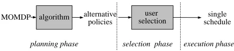
[image:3.612.54.289.53.105.2]selection phase planning phase
Figure 1:Decision support for MOMDPs
element of this set would be most preferred (Clemen 1997). Such a scenario is called decision support, i.e., the actual val-ues for alternativesVπ are input to the discussion between human decision makers (Clemen 1997), as illustrated in Fig-ure 1. In this case, we need an MOMDP method that returns the best possible valueVπfor each possiblew, from which
in theselection phasehuman decision makers can select one to execute.
The solution to an MOMDP for linear scalarisations is called the convex coverage set (CCS)2,3
CCS=nVπ:∃w∀π0w·Vπ≥w·Vπ0o.
We assume that all objectives are desirable, i.e., all weights are positive. And, because only relative importance between the objectives is important when computing optimal solu-tions, we assume without loss of generality that the weights lie between0and1and sum to1. To compute the CCS we can thus restrict ourselves to weights on a simplex (see Fig-ure 2).
In order to find the CCS we can make use of specialised algorithms. One such method is optimistic linear support
(Roijers, Whiteson, and Oliehoek 2014) which was origi-nally proposed for multi-objective coordination graphs but can be applied to MOMDPs as well. OLS requires a sub-routine that solves a linearly scalarised version of a problem exactly. We first explain OLS and known MDP techniques that we use to form an MOMDP method.
2.3
Optimistic Linear Support
Roijers, Whiteson, and Oliehoek (2014) propose a CCS al-gorithm calledoptimistic linear support(OLS), that works by computing the exact solution to weighted MDPs for specifically chosen weights by scalarising a multi-objective decision problem and running a single-objective solver. They show that the single-objective method only needs to be called for a finite number of weights in order to obtain the exact CCS. In order to see why only a finite number of weights are necessary to compute the full CCS, we first need to define the scalarised value function:
VCCS∗ (w) = max
Vπ∈CCSw·V
π,
and note that this is apiecewise-linear and convex(PWLC) function. Note that we only need to define this function on the weight simplex. We plot the PWLC functionVCCS∗ of
2
The convex coverage set is often called theconvex hull. We avoid this term because it is imprecise: the convex hull is a superset of the convex coverage set.
3
The CCS is a subset of the Pareto front. Please refer to (Roijers et al. 2013) for an extensive discussion on both.
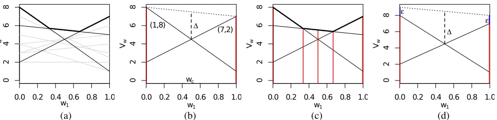
a two-objective problem as a function of the weight for the first objective in Figure 2a. Because the scalarisation is lin-ear, the value of a policy becomes a line. The functionV∗
CCS
is indicated by the bold line segments.
OLS builds the CCS incrementally from an initially empty partial CCS, S, adding vectors that are optimal for specific weights on the weight simplex. In order to find the optimal solution for a specific weight, OLS runs an ex-act single objective solversolveMDPon an instance of the MOMDP scalarised usingw.S contains the known value vectors, i.e., the vectors we know are definitely in the CCS. The scalarised value function overS is defined similarly as the one for the complete CCS:VS∗(w) = maxVπ∈Sw·Vπ,
and again, is PWLC.
OLS starts by looking at the extrema of the weight sim-plex. Figure 2a shows the two value vectors found at the ex-trema of the weight simplex of a 2-objective example. The weights at which the vectors are found are indicated with bold red vertical lines. The area above the functionVS∗(w)
is a polyhedron (Bertsimas and Tsitsiklis 1997) whose ver-tices correspond to unique weights called corner weights. Using only the corner weights, OLS can find the exact CCS. This is possible due to a theorem by Cheng (1988) that states that there is a corner weight ofVS∗(w)that maximises
∆(w) = VCCS∗ (w)−VS∗(w), i.e., the maximal improve-ment ofS that can be made by adding a value vector to it, with respect to the true CCS, is at one of the corner weights. This results from two observations: the values at the cor-ner weights of VS∗(w) are smaller than or equal to those of VCCS∗ (w)by definition and S ⊆ CCS. Therefore the maximal error can only be in a region for which the op-timal vector is not in S. Under this region the difference
VCCS∗ (w)−VS∗(w)is a concave function, with identical cor-ner weightsVS∗(w)that hence necessarily specify the unique maximum for these regions.
Because of Cheng’s theorem, if all the corner points are checked and no improvement has been found, the residual error must be zero. OLS checks the corner weights of S, prioritising on maximal possible improvement. As the ex-act CCS is unknown, OLS measures the maximal possi-ble improvement with respect to the most optimistic hypo-thetical CCS,CCS, that is still consistent withS, and the valuesVS∗(w)at the weights where the vectors in S have been found (at these weights OLS knows that VS∗(w) = VCCS∗ (w) =V∗
CCS(w)).
(a) (b) (c) (d)
Figure 2: (a) All possible value vectors for a 2-objective MOMDP. (b) OLS finds two payoff vectors at the extremaw= (0,1)
andw= (1,0), a new corner weightwc = (0.5,0.5)is found, with maximal possible improvement∆.CCSis shown as the
dotted line. (c) OLS finds a new vector at(0.5,0.5), resulting in two new corner points which do not result in new vectors, makingS=CCS=CCS. (d) AOLS computes the priorities using an adjusted optimistic CCS.
3
Approximate Optimistic Linear Support
OLS can find the exact CCS only when we can find exact solutions for all weights. This is an important limitation, be-cause it is often computationally infeasible to compute exact solutions for the (often large) MDPs used to model stochas-tic planning problems. In this section, we propose approx-imate OLS(AOLS), which does not require an exact MDP solver. Because AOLS employs approximate MDP solvers, the so-called corner weights need to be recomputed every-time we find a new value vector, which is not necessary in OLS. Furthermore, the computation of maximal possible er-ror and the next weight for which to call the MDP solver are different from OLS. We establish both a convergence guar-antee and show that AOLS provides a bounded approxima-tionover all weights.
First, we assume that instead of an exact algorithm for
solveMDPwe have an- approximate algorithm.
Definition 1. An-approximate MDP solveris an algorithm that produces a policy, whose expected value is at least(1− )V∗, whereV∗is the optimal value for the MDP and≥0.
Given an-approximate MDP solver we can compute a set of policies for which the scalarised value for each possi-blewis at most a factoraway from the optimum (-CCS). In Section 3.2 we show that AOLS can still be applied even without this assumption, though with weaker guarantees.
AOLS, shown in Algorithm 1, takes as input an MOMDPM, and a single objective MDP solversolveMDP
that is-approximate. AOLS maintains the set of value vec-tors and associated policies in a setS(initialised on line 1). It keeps track of the tuples of weights already searched with their corresponding scalarised values (initialised on line 2). AOLS starts by selecting the first extremum (the unit vec-tore1, e.g.(0,1)or(1,0)in the two-objective case) of the weight simplex with an infinite maximal possible improve-ment (line 3 and 4). Until there is no corner weight with a maximal relative improvement of at least left (line 5), AOLS scalarises the MOMDP M with weightwmax and
computes an -optimal policy π(line 6). AOLS then uses policy evaluation to determine the expected value of said policy (line 7) (Bellman 1957b). This evaluation step can be expensive, but is usually much less expensive than finding an
Algorithm 1:AOLS(M,solveMDP, ) Input: An MDP
1 S← ∅//partial CCS
2 W Vold← ∅//searched weights and scalarised values
3 ∆max← ∞
4 wmax←e1
5 while∆max> ∧ ¬timeOutdo
6 π←solveMDP(scalarise(M,wmax))
7 Vπ←evaluatePolicy(M,π)
8 W Vold=W Vold∪ {(wmax, wmax·Vπ)}
9 ifVπ6∈Sthen 10 S←S∪ {Vπ}
11 W ←recompute corner weightsVS∗(w) 12 (wmax,∆max)←calcOCCS(S, W Vold, W, )
13 end 14 end
15 returnS,∆max
(-)optimal policy. After computing the value, the searched weight and corresponding scalarised value is added to the setW Vold(line 8), which is necessary to compute the
opti-mistic CCS.
If the vectorVπfound atwmaxis new, i.e., not inS, it is
added to this solution set (line 10). However, because these values are approximate values, it is not certain that they are optimal anywhere. Therefore, contrary to OLS, we need to test whether any of the vectors inS∪ {Vπ}is dominated,
and recompute all the corner weights accordingly (line 11). This recomputation can be done by solving a system of lin-ear equations. For all corner weights, we compute the max-imal possible improvement∆(w) = V∗
CCS(w)−V
∗
S(w).
This happens in Algorithm 2, in which for each corner weight,∆(w)is evaluated, using a linear program.
The definition of the optimistic CCS is different than the CCS used in OLS because it incorporates the possibility of being -wrong, shifting the scalarised value V∗
CCS(w)
upwards (as shown in Figure 2d). The maximal scalarised value of V∗
CCS(w)for a givenwcan be found by solving
the linear program given on line 6 in Algorithm 2. This lin-ear program is different than that of OLS, because of the
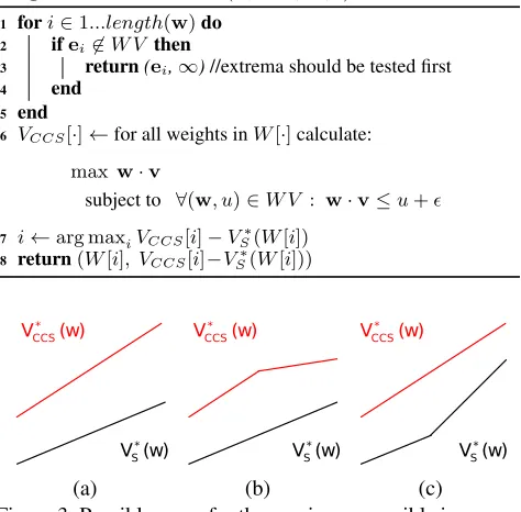
[image:4.612.69.553.56.173.2]Algorithm 2:calcOCCS(S, W V, W, ) Input: An MDP
1 fori∈1...length(w)do 2 ifei6∈W V then
3 return(ei,∞)//extrema should be tested first
4 end 5 end
6 VCCS[·]←for all weights inW[·]calculate:
max w·v
subject to ∀(w, u)∈W V : w·v≤u+
7 i←arg maxiVCCS[i]−VS∗(W[i])
8 return(W[i], VCCS[i]−VS∗(W[i]))
[image:5.612.56.293.69.302.2](a) (b) (c)
Figure 3: Possible cases for the maximum possible improve-ment ofSwith respect to theCCS.
anytime algorithm, i.e., the highest value of∆(w)is the cur-rentof an-CCS.
3.1
Correctness
We now establish the correctness of AOLS. Because the scalarised value ofV∗
CCS(w)(as computed by Algorithm 2)
obtained through using theof the approximatesolveMDP
is no longer identical toVS∗(w), we need to make an adjust-ment to Cheng’s theorem.
Theorem 1. There is a corner weight ofVS∗(w)that max-imises:
∆(w) =VCCS∗ (w)−VS∗(w),
whereSis an intermediate set of value vectors computed by AOLS.
This theorem is identical in form to Cheng’s, but, becauseS
is no longer a subset ofCCS, the proof is different.
Proof. ∆(w)is a PWLC function because it is constructed as the difference between two PWLC functions. To max-imise this function, we have three possible cases, shown in Figure 3: (a) the maximum is at a weight that is neither a corner point ofV∗
CCS(w), nor ofVS∗(w); (b) it is at a corner
point ofVCCS∗ (w)but not ofVS∗(w); or (c) it is at a corner point ofVS∗(w).
Case (a) only applies if the slope of∆(w)is 0, and there-fore the value is never higher than the value at the corner points where this slope changes. Case (b) can never occur, because if w is a corner point of CCS, and not of S, and
VCCS∗ (w)−VS∗(w)is at a maximum, thenVCCS∗ (w)must be at a maximum atw. IfVCCS∗ (w)is at a maximum at a weightw then it cannot be a PWLC function, leading to a contradiction. Therefore, only case (c) remains.
Because the maximum possible improvement is still at the corner points of S, even though S now contains
-approximate solutions, the original scheme of calling
solveMDPfor the corner weights still applies.
AOLS terminates when the maximal possible improve-ment is smaller than or equal to ·V∗
CCS(w), i.e., corner
weights with a possible improvement less than that are no longer considered.
Theorem 2. AOLS terminates after a finite number of calls to an-approximate implementation ofsolveMDPand pro-duces an-CCS.
Proof. AOLS runs until there are no corner points left in the priority queue to check, and returns S. Once a corner point is evaluated, it is never considered again because the established value lies within(1−)V∗
CCS(w). AOLS thus
terminates after checking a finite number of corner weights. All other corner weights have a possible improvement less thanVCCS∗ (w). ThereforeSmust be an-CCS.
3.2
Unbounded Approximations
When thethatsolveMDPguarantees is known, Theorem 1 guarantees an-CCS. WhensolveMDPuses an approximate implementation where is not known beforehand, AOLS still converges on some approximation of the CCS. but, sinceis unknown, it cannot prioritise which corner weight to check first. Therefore, ∆max cannot be computed, and
AOLS selects a random yet unchecked corner weight. In this case. AOLS cannot guarantee a certain . In Section 5, we use such an implementation (PROST) and determine the
empirically by comparing against an exact implementation ofsolveMDP(SPUDD).
4
Scalarised Sample-based Incremental
Improvement
If no a priori information about the weights is known, the AOLS algorithm can successfully approximate the CCS for all possible weights and, when the single-objective subrou-tine is bounded, AOLS provides an-CCS. However, deci-sion makers can often provide an indication as to the prefer-ences they might have. We can expression this information using a prior distribution over the weights that we can ex-ploit, e.g., if they cannot exactly specify the economic im-pact of delay but instead know a distribution over its poten-tial impact cost.
In such scenarios, AOLS might not be the best approach since it distributes its planning effort equally over the cor-ner weights (which might not be in the right region), i.e., the allowed time budget for the single objective planner for each corner weight is the same. Approximate single objec-tive methods such as UCT* provide better approximations when given more time. If we can focus on important weights we may be able to establish a betterin the regionswhere it matters most, and as a result discover more relevant avail-able trade-offs than possible without a prior.
Algorithm 3:SSII(M,solveMDP, pr, N, timeOut) Input: An MOMDPM, a priorprover the weights, an
number of samplesN
1 weightsList←sampleNweights frompr 2 fori∈[1...N]do
3 ti←minimum runtimesolveMDP
4 vectorList[i]←runsolveMDP(m, weightsList[i], ti)
5 end
6 while¬timeOutdo
7 (wmax,∆max)←
calcOCCS(vectorList, weightsList, )
8 getifor whichwmax=weightsList[i]and increaseti
9 vectorList[i]←cont.solveMDP(M, weightsList[i], ti)
10 end
11 returnvectorList
most interesting regions. The algorithm takes as input the MOMDPM, an anytime single objective solversolveMDP, a prior distribution over weights pr, the number of sam-plesN, and a timeouttimeOut; it produces an optimistic CCS.
For each weightwsampled from the prior distributionpr, the algorithm quickly computes an initial approximate pol-icy and associated value vectorVˆπw(lines 1-5). After
deter-mining this initial set of value vectors, it improves on the ex-pected reward by incrementally allowing the anytime solver more runtime to improve the solution for one sample at a time (lines 6-10). Note that we abuse the notation of the call tocalcOCCS, the argumentW V is composed ofvectorList
andweightsList, and S is justvectorListandW is just
weightsList.
The incremental improvement per sample is guided by a procedure that prioritises these weight samples. At each it-eration, one sample is selected, and SSII will continue to improve until a specified time limit has been reached for the runtime of the single objective MDP solver (line 9). Improv-ing on one of vectors by runnImprov-ingsolveMDPdoes not require a full rerun; insteadsolveMDPsaves its state and resumes from there. In UCT*, we can preserve the search tree and continue from there if an improvement of the same sample weight is required.
Selecting which sampled weight w to improve can be done in various ways, yielding different anytime and final solutions. Our implementation of SSII prioritises the sam-ples based on their improvement∆(w)as defined in the pre-vious section. Intuitively, this will focus the SSII algorithm on samples with the highest potential improvement.
5
Experiments
In this section, we present an empirical analysis of the per-formance of the AOLS and SSII algorithms in terms of both runtime and quality of the CCS. In order to illustrate the run-time difference with exact methods, we compare against the exact OLS/SPUDD algorithm. Both AOLS and SSII use the UCT* algorithm to approximate policies. Because we can-not let UCT* run until all states have been evaluated, we can only obtain a partial policy. In our experiments we ‘repair’ partial policies, i.e., supplement these policies by taking a conservative action; in the problems we consider this means inserting no-ops and corresponding result states (see next
section), thereby not changing the expected value of the pol-icy. Note that one could use any heuristic to supplement the partial policies.
Our experiments are performed on themaintenance plan-ning problem(MPP) (Scharpff et al. 2013). Using generated instances of this problem, we measure the error with respect to the exact CCS. The experiments use a JAVA implemen-tation that calls the SPUDD and PROST packages.4All ex-periments were conducted on an Intel i7 1.60 GHz computer with 6 GB memory.
5.1
Maintenance Planning
Themaintenance planning problemconsists of a set of con-tractors, i.e. the agents, N and a period of discrete time stepsT = [t1, t2, . . . , th]wherehis the horizon length.
Ev-ery agenti ∈N is responsible for a setAi of maintenance
activities. The main goal in this problem is to find a contin-gent maintenance schedule that minimises both the cost as well as the traffic hindrance.
The maintenance activities a ∈ Ai are defined by
tu-pleshw, d, p,dˆiwherew ∈ R+ is the payment upon com-pletion of the task, d ∈ Z+ is the number of consecutive time steps required to complete the task,p∈[0,1]the prob-ability that a task will delay and dˆ ∈ Z+ the additional duration if the task is delayed. Each agent also has a cost functionci(a, t)that captures the cost of maintenance (e.g.
personnel, materials, etc.) for all of its activitiesa∈Aiand
every time stept ∈T. Agents are restricted to executing at most a single maintenance activity and they can only plan activities if they are guaranteed to finish them within the plan horizon. The utility of an agent is defined by the sum of payments minus the costs for every completed activity and therefore depends on the executed maintenance schedulePi.
When we assume thatPicontains for each time stept∈T
the activity that was executed we can write this utility as
ui=Pai∈Piwai− P
t∈Tc(Pi(t), t).
The impact of maintenance on the network throughput is given by the function `(At, t), expressed in traffic time lost (TTL). In this function, At is used to denote any
combination of maintenance activities being performed at timet, by one or more agents. This function allows us to employ arbitrary models, e.g., extrapolated from past re-sults, obtained through (micro-)simulation or computed us-ing heuristic rules.
We model the MPP as an MOMDP in which the state is defined as the activities yet to be performed, the time left to perform them, and the availability of the individual agents. Because the agents arecooperative we can treat the set of agents as a single agent: the actions at each time step are the possible combinations of actions that could be started at that time step, i.e., the Cartesian product of the possible actions for each agent. The activities have an uncertain completion time, as maintenance activities can run into delays, result-ing in a stochastic transition function. The reward is of the formP
i∈Nui−
P
t`(A t, t)
4
These can be found at www.computing.dundee.
ac.uk/staff/jessehoey/spudd/ and prost.
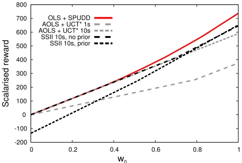
Figure 4:Typical example of solution sets found by AOLS, SSII and OLS/SPUDD, using different runtimes.
For our experiments, we generated many instances of the problem with various sizes. All of them arefully coupled, i.e., for each pairai ∈Ai, aj ∈ Aj there exists a network
cost`(ai, aj)>0.
5.2
CCS Quality Metrics
The error of the coverage sets obtained through AOLS and SSII is defined with respect to the actual CCS (ob-tained through OLS/SPUDD). We describe the output sets of AOLS or SSII as S, and the actual CCS asCCS. We define two error metrics: maximal and expected error.
The maximal error εmax is a conservative measure that
specifies the maximal scalarised error over all possiblew. This measure does not include any prior information over the weights:
εmax(S, VCCS∗ ) = max
w V
∗
CCS(w)−VS∗(w).
Note that this metric is absolute rather than relative. The expected error incorporates the prior distribution overw,prin order to give a larger penalty to errors in more important regions:
εexp(S, VCCS∗ ) =
Z
w
pr(w)(VCCS∗ (w)−VS∗(w))dw.
5.3
Comparison of Algorithms
In order to test the performance of AOLS and SSII in terms of runtime and solution quality, we apply these algorithms to the MPP domain. We take moderately sized instances so that it is possible to find the exact CCS for compari-son. To compute the exact CCS, we apply OLS with ex-act solutions found by SPUDD (Hoey et al. 1999) as the exact single-objective MDP solver subroutine. The approxi-mation of policies for both AOLS and SSII is done using the UCT* algorithm from the PROST toolbox (Keller and Eye-rich 2012). UCT* is an anytime algorithm which is expected to perform better when it is given more time to compute ap-proximate solutions. Therefore, we test AOLS and SSII with various settings for the allowed runtime for UCT*. For SSII we ran both experiments with and without prior knowledge
about weights. We use limited information of the form “costs are more important than TTLs” leading to a uniform prior in a limited range of weights,[0.5,1]for the cost weight (and hence[0,0.5]for the TTL weight).
To develop an intuition on the quality of the solution sets found by AOLS and SSII for varying runtimes, we first test them on a single test problem, with two maintenance compa-nies and three activities each, and visualise the resulting so-lution setsSby plottingVS∗(w), as shown in Figure 4. SSII was given a uniform prior on the interval [0.5,1]. For low runtimes we observe that AOLS is better than SSII where the prior has probability mass 0, i.e.,w1 <0.5, but SSII is better in the region it focuses on. For higher runtimes, AOLS and SSII both happen to find a good vector for the left side of the weight space, and both methods find the same value forw1= 0.5.
Neither AOLS nor SSII achieves the value of the exact CCS with their solution sets. However, much less runtime was used compared to finding the optimum. OLS/SPUDD used around 3 hours, while AOLS used close to 6 minutes, and SSII just over 7 minutes, both with10sallowed for the single objective solver.
In order to test the error with respect to the CCS numer-ically, we averaged over 12 MPP instances with 2 mainte-nance companies with 3 activities each with randomly (uni-formly) drawn horizons between 5 and 15. Table 1 shows the average performance per algorithm, expressed in terms ofεmax,εexpand the fraction of instances solved optimally.
The exact solver was run once for each problem, whereas the AOLS and SSII algorithms were run 5 times on the same problem to compute the average performances and runtimes, because UCT* is a randomised algorithm.
These results show a striking difference between the ex-act and approximation runtimes. Whereas the average run-time required to find the optimum CCS is in the range of hours (the longest took 3.5 hours), SSII and AOLS require time in the order of seconds to a few minutes to find an op-timistic CCS. Moreover, our experiments confirm that the maximal and expected errors decrease when more runtime is given. Also very interesting is that both AOLS and SSII are able to find a (near-)optimal CCS in many cases, where OLS takes hours to do the same, and that SSII is competitive with AOLS.
In order to demonstrate that prior information on the dis-tribution over the weight can be exploited, we ran SSII with two different sample ranges. ‘SSII no prior’ used 5 evenly distributed samples over the entire region, i.e., assuming no prior information is available. The ‘SSII prior’ algorithm, also distributed its samples evenly, but only in the range
[0.5,1]. Note that any CCS found with samples in this range is also a CCS for the full weight range, although not likely to be close to optimal outside the sample range. The results in the last three columns show the errors for only the range of the prior, illustrating that both the maximal error, expected error and even the percentage of optimal solutions found
[0,1] [0.5,1]
Algorithm Runtime |CCS| εexp εmax %OPT εexp εmax %OPT
OLS + SPUDD 2390.819 9.250 - - -
[image:8.612.91.525.51.191.2]-AOLS + UCT* 0.01s 8.612 3.389 0.701 325.354 0.000 0.692 325.025 0.000 AOLS + UCT* 1s 19.940 4.111 0.119 65.668 0.167 0.117 65.426 0.167 AOLS + UCT* 10s 65.478 4.528 0.084 56.439 0.333 0.091 56.381 0.333 AOLS + UCT* 20s 165.873 5.694 0.044 38.667 0.417 0.048 38.627 0.417 SSII 1s, no prior 18.795 4.306 0.118 70.244 0.167 0.116 70.195 0.167 SSII 10s, no prior 59.336 3.889 0.061 51.800 0.333 0.068 51.747 0.333 SSII 1s, prior 17.892 3.944 0.221 95.189 0.000 0.125 61.667 0.167 SSII 10s, prior 59.154 4.083 0.141 71.290 0.083 0.057 43.006 0.333
Table 1: Comparison of averaged performance of the algorithms presented in this paper for various parameters, shown for two regions of the scalarised reward space. Runtimes are in seconds, the expected errorεexpand maximum errorεmaxare relative
to the optimum CCS and %OPT denotes the fraction of instances that were solved optimally.
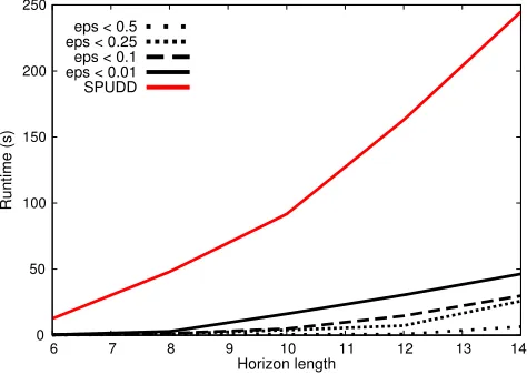
Figure 5:Average runtime for UCT* to attain variouslevels and the runtime required to compute the optimal policy using SPUDD.
5.4
UCT* approximation quality
Although the UCT* algorithm does not provide a guarantee on the resulting policy value, we establish empirically that, given sufficient runtime, it can produce-approximations for various values of. Using the same instances as before, we determine the average runtime that is required to obtain such approximation levels. For each instance, we run the UCT* algorithm 10 times, where we iteratively increase the al-lowed runtime in each run until a solution of the required quality is obtained. Figure 5 shows the average runtimes in seconds required to obtain various compared to the run-time of SPUDD, for different horizon lengths. From the fig-ure we can see that UCT* obtains at least half of the optimal value within mere seconds. Interestingly, UCT* is also able to produce near-optimal solutions within a minute for these problem instances (sometimes the optimum is found, see Ta-ble 1). Unfortunately, we do not know whether these results translate to larger problem sizes, as a comparison with exact solutions is computationally infeasible for bigger problems.
6
Related Work
Several other methods exist for computing the CCS MOMDPs. Viswanathan, Aggarwal, and Nair (1977)
de-vise a linear programming method for episodic MOMDPs; Wakuta and Togawa (1998) use a policy iteration based method and Barrett and Narayanan (2008) extend value iter-ation with CCS computiter-ations in the back-up phase to form convex hull value iteration (CHVI). However, unlike our ap-proach, all these methods assume the state space is small enough to allow exact solution. Moreover, they deal with the multiple objectives on a low level, deep inside the algo-rithms. In contrast, we deal with the multiple objectives in a modular fashion, i.e., both AOLS and SSII have an outer loop to deal with the multiple objectives and call approxi-mate single-objective MDP solvers as a subroutine. We can thus easily replace these subroutines with any future method. The closest MOMDP method to our work is Li-zotte, Bowling, and Murphy (2010)’s finite-horizon multi-objective value iteration algorithm for continuous state-spaces, and its extended version (Lizotte, Bowling, and Mur-phy 2012). This method plans backwards from the plan-ning horizon, computing a point-based (i.e., using sampled weights) value backup for each timestep until t = 0 is reached. However, their approach is infeasible in our setting because of the large number of reachable end states. Instead, UCT* performs a forward Monte-Carlo tree search starting att= 0, reducing the number of end states visited.
7
Conclusions and Future Work
Solving MDPs with multiple objectives is challenging when the relative importance of objectives is unclear or impossi-ble to determine a priori. When MOMDPs can be linearly scalarised, we should find the set of alternatives – the con-vex coverage set – which for each choice of weight span the maximal achievable expected rewards. Finding the exact convex coverage set is however often not feasible, because finding exact solution of a (single-objective) MDP is already polynomial in the number of states, and the number of states in many problems is huge. In this work we therefore focused on methods to approximate the CCS for MOMDPs.
[image:8.612.55.292.239.408.2]an approximation method to compute the multi-objective value at corner weights (Theorem 1). Moreover, when an
-approximation algorithm is used, we can bound the loss in scalarised value of the resulting approximate CCS.
Although AOLS is generally applicable, it cannot exploit prior information on the distribution of weights. When such a prior is available we want to focus most of our attention to the regions of the CCS that correspond to this distribution. Instead, SSII samples weights from this prior for which it it-eratively tries to improve the policy, prioritising the samples that are the furthest away from the best known CCS.
We compared the performance of the approximate algo-rithms proposed in this paper with the optimal algorithm in terms of runtime, expected CCS error and maximum CCS error, on problems from the maintenance planning domain (Scharpff et al. 2013). These experiments show that both al-gorithms can compete with the exact algorithm in terms of quality, but require several orders of magnitude less runtime. When a prior is known, our experiments show that SSII has a slight advantage over AOLS.
In this paper, we assume that it is feasible to perform exact evaluation ofVπ, i.e., the multi-objective value. In MPP this
assumption appears valid. In general, however, this also be-comes an expensive operation for large problems. An impor-tant direction of future research, therefore, is to investigate if it is possible to extend our results to the case of approximate evaluation ofVπ.
Another direction for future work is to combine the two main ideas presented in this work for cases when no single objective solver with a knownbound is available. We are interested in improving the performance of AOLS by apply-ing a heuristic exploitapply-ing a prior on the weights to decide on which corner point to evaluate.
This work assumes that the agents are fully cooperative, but many problems exists where this is not the case. For in-stance in the MPP domain, when agents are self-interested they will not likely give up profits in favour of traffic hin-drance reduction unless they are explicitly motivated to do so. A mechanism design approach, similar to (Scharpff et al. 2013), could help to extend this work to the wider class of non-cooperative planning problems.
Acknowledgements
This research is supported by the NWO DTC-NCAP
(#612.001.109), Next Generation Infrastructures/Almende BV and NWO VENI (#639.021.336) projects.
References
Alarcon-Rodriguez, A.; Haesen, E.; Ault, G.; Driesen, J.; and Belmans, R. 2009. Multi-objective Planning Frame-work for Stochastic and Controllable Distributed Energy Re-sources.IET Renewable Power Generation3(2):227–238. Barrett, L., and Narayanan, S. 2008. Learning All Optimal Policies with Multiple Criteria. InProc. of the International Conference on Machine Learning, 41–47. New York, NY, USA: ACM.
Bellman, R. E. 1957a. A Markov Decision Process.Journal of Mathematical Mechanics6:679–684.
Bellman, R. E. 1957b. Dynamic Programming. Princeton, NJ: Princeton University Press.
Bertsimas, D., and Tsitsiklis, J. 1997.Introduction to Linear Optimization. Athena Scientific.
Calisi, D.; Farinelli, A.; Iocchi, L.; and Nardi, D. 2007. Multi-objective Exploration and Search for Autonomous Rescue Robots.Journal of Field Robotics24(8-9):763–777. Cheng, H.-T. 1988. Algorithms for Partially Observable Markov Decision Processes. Ph.D. Dissertation, UBC. Clemen, R. T. 1997. Making Hard Decisions: An Intro-duction to Decision Analysis. South-Western College Pub, 2 edition.
Hoey, J.; St-Aubin, R.; Hu, A.; and Boutilier, C. 1999. SPUDD: Stochastic Planning Using Decision Diagrams. In
Proc. of the Fifteenth conference on Uncertainty in artificial intelligence, 279–288.
Keller, T., and Eyerich, P. 2012. PROST: Probabilistic Plan-ning Based on UCT. InProc. of the International Confer-ence on Automated Planning and Scheduling.
Keller, T., and Helmert, M. 2013. Trial-based Heuristic Tree Search for Finite Horizon MDPs. In Proc. of the Interna-tional Conference on Automated Planning and Scheduling. Lizotte, D. J.; Bowling, M.; and Murphy, S. A. 2010. Effi-cient Reinforcement Learning with Multiple Reward Func-tions for Randomized Clinical Trial Analysis. In27th Inter-national Conference on Machine Learning, 695–702. Lizotte, D. J.; Bowling, M.; and Murphy, S. A. 2012. Linear Fitted-Q Iteration with Multiple Reward Functions. Journal of Machine Learning Research13:3253–3295.
Mouaddib, A.-I. 2004. Multi-objective Decision-theoretic Path Planning. InProc. of the International Conference on Robotics and Automation, volume 3, 2814–2819. IEEE. Roijers, D. M.; Vamplew, P.; Whiteson, S.; and Dazeley, R. 2013. A Survey of Multi-Objective Sequential Decision-Making. Journal of Artificial Intelligence Research47:67– 113.
Roijers, D. M.; Whiteson, S.; and Oliehoek, F. 2014. Linear Support for Multi-Objective Coordination Graphs. InProc. of the Autonomous Agents and Multi-Agent Systems confer-ence.
Scharpff, J.; Spaan, M. T. J.; Volker, L.; and de Weerdt, M. 2013. Planning Under Uncertainty for Coordinating Infras-tructural Maintenance. Proc. of the International Confer-ence on Automated Planning and Scheduling.
Vamplew, P.; Dazeley, R.; Berry, A.; Issabekov, R.; and Dekker, E. 2011. Empirical Evaluation Methods for Mul-tiobjective Reinforcement Learning Algorithms. Machine Learning84(1-2):51–80.
Viswanathan, B.; Aggarwal, V. V.; and Nair, K. P. K. 1977. Multiple Criteria Markov Decision Processes.TIMS Studies Management Science6:263–272.
Wakuta, K., and Togawa, K. 1998. Solution Procedures for Markov Decision Processes. Optimization: A Journal of Mathematical Programming and Operations Research