Three Dimensional Electrical Impedance Tomography

This is a repository copy of Three Dimensional Electrical Impedance Tomography. White Rose Research Online URL for this paper:

http://eprints.whiterose.ac.uk/424/

Article:

Metherall, P., Barber, D.C., Smallwood, R.H. [r.smallwood@shef.ac.uk] et al. (1 more author) (1996) Three Dimensional Electrical Impedance Tomography. Nature, 380 (6574). pp. 509-512. ISSN 0028-0836

https://doi.org/10.1038/380509a0

eprints@whiterose.ac.uk https://eprints.whiterose.ac.uk/

Reuse

Unless indicated otherwise, fulltext items are protected by copyright with all rights reserved. The copyright exception in section 29 of the Copyright, Designs and Patents Act 1988 allows the making of a single copy solely for the purpose of non-commercial research or private study within the limits of fair dealing. The publisher or other rights-holder may allow further reproduction and re-use of this version - refer to the White Rose Research Online record for this item. Where records identify the publisher as the copyright holder, users can verify any specific terms of use on the publisher’s website.

Takedown

If you consider content in White Rose Research Online to be in breach of UK law, please notify us by

Three-dimensional electrical impedance tomography

Metherall, P.; Barber, D. C.; Smallwood, R. H.; Brown, B. H.

Abstract

The electrical resistivity of mammalian tissues varies widely (1-5) and is correlated with physiological function (6-8). Electrical impedance tomography (EIT) can be used to probe such variations in vivo, and offers a non-invasive means of imaging the internal conductivity distribution of the human body (9-11). But the computational complexity of EIT has severe practical limitations, and previous work has been restricted to considering image

reconstruction as an essentially two-dimensional problem (10,12). This simplification can limit significantly the imaging capabilities of EIT, as the electric currents used to determine the conductivity variations will not in general be confined to a two-dimensional plane (13). A few studies have attempted three-dimensional EIT image reconstruction (14,15), but have not yet succeeded in generating images of a quality suitable for clinical applications. Here we report the development of a three-dimensional EIT system with greatly improved imaging capabilities, which combines our 64-electrode data-collection apparatus (16) with customized matrix inversion techniques. Our results demonstrate the practical potential of EIT for clinical applications, such as lung or brain imaging and diagnostic screening (8).

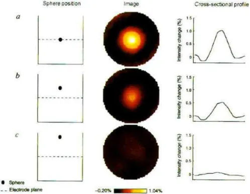
Our methodology of two-dimensional (2D) EIT has been described in detail previously (10,12,17). Electrodes are positioned with equal spacing around the body to be imaged, thus defining a plane through the object. Voltage profiles are collected for all drive and receive electrode-pair combinations, and images are reconstructed as though the data were from a 2D object. In practice objects are three-dimensional (3D) and figure 1 shows 2D images obtained from such an object. These demonstrate that there are significant contributions to the image from off-plane conductivity changes. This means that, unlike 3D X-ray images which can be constructed from a set of independent 2D images, for 3D EIT it is necessary to reconstruct images from data collected over the entire surface of the object volume (12).

Figure 1. Images showing how off-plane conductivity changes affect the reconstructed image in 2D EIT. As the conductivity change is moved further away from the electrode plane, its intensity in the image plane falls. But changes at distances equal to the tank (phantom) radius can still be resolved in the image plane. Radially offset changes show a similar effect, but with the further complication that off-plane changes are also shifted towards the centre of the image (13). All three images are displayed using the colour scale shown. The maximum values of conductivity change, expressed as a percentage, are given. METHODS. The images were produced using a 16-electrode system with interleaved drive and receive electrodes (16). Current is driven through a pair of electrodes into the body and potential differences are measured between the other electrode pairs. The current drive pair is then rotated and another set of voltage measurements is

-1) and a reference (gref) voltage profile was collected. A small electrically insulating sphere of diameter 20 mm

was then positioned as follows: a, in the electrode plane; b, at a distance of half the phantom radius from electrode plane; and c, at a distance of the phantom radius from electrode plane. Data sets (g) were recorded for each position, and the boundary voltage profile is then given by Delta gn = (g - gref)/gref.

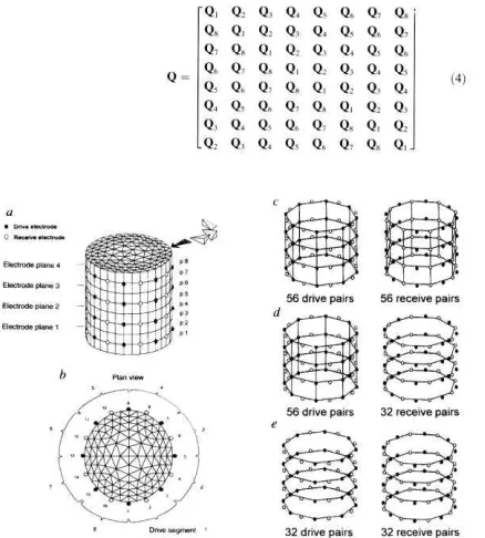
In this work we have taken a sample of the boundary surface using 64 electrodes placed around the object (32 independent current drive and 32 voltage receive channels), figure 2. Current is driven between pairs of adjacent drive electrodes. For each drive pair, a set of voltage measurements are recorded from receive electrode pairs. Three data collection strategies have been studied to investigate the performance of image reconstruction with different boundary voltage data set sizes. These sequences were derived from knowledge of limitations in the data collection instrumentation (16) and are shown in figure 2.

Figure 2. Three-dimensional mesh, electrode position and pair configuration. To generate the reconstruction algorithm, a model representing the object volume is divided into 4,608 tetrahedral elements. These are configured as eight planes of 576 elements (a). On nodes at the surface of the cylinder, the electrode positions are shown. This is based on a 64-electrode data collection system with 32 independent current drive and voltage

measurement (receive) electrodes. They are arranged in four planes of 16, with an interleaved configuration. METHODS. Three data collection sequences were studied with different data set sizes. The first (c) includes 56 drive and 56 receive pairs, formed between electrodes in the same plane and between adjacent planes (Delta gn = 3,136

elements); the second (d) has only 32 in-plane receive pairs (Delta gn = 1,792 elements) and the

third (e) has 32 drive and 32 receive pairs (Delta gn

= 1,024 elements). The ordering of the data collection sequence is configured so that we have rotational symmetry. Current is first driven sequentially between pairs on all planes

corresponding to drive segment 1, with a full set of voltage measurements collected for each drive pair. Current is then driven between pairs in segment 2, but the order of voltage measurements is shifted so that the

geometrical relationship between the receive pairs and the drive pairs is identical for each segment (b).

In order to generate the reconstruction algorithm, we have split the volume of interest into 4,608 tetrahedral elements. A sensitivity matrix, based on the theorem by Geselowitz (18,19), can be derived which relates the magnitude of small changes in conductivity, Delta c = c - cref,

and the resulting changes in potential differences Delta g = g - gref, on the boundary of the

object, by equation 1. Although the sensitivity matrix S changes with the conductivity distribution and is therefore nonlinear, for small changes in c this can be ignored (12). We have argued elsewhere (20) that it is preferable to replace the perturbed data Delta g by a set of potential differences normalized to the reference vector gref and in this case equation (1)

becomes equation 2 where Delta gn is the normalized change in boundary voltages and Delta

cn is the normalized change in conductivity.

Equation 1

Matrix F is now the normalized sensitivity matrix in which the coefficient corresponding to a particular drive/receive pair and tetrahedral element is normalized by the sum of coefficients for the same drive/receive pair over all the elements. Although F is no better conditioned than S, it is less dependent on the requirements of a circular boundary shape and accurate electrode positioning (12,20). This is essential for clinical imaging applications, where a subject's profile does not match the model used to generate the sensitivity matrix and accurate placement of electrodes is difficult.

Inverting the above relationship (equation 2) allows us to reconstruct the internal change in conductivity, Delta cn, from measured boundary data. Sensitivity coefficients, S, are formed

for each tetrahedral element and for all drive/receive electrode-pair combinations. Del phid is

the potential gradient that is generated within a tetrahedral element (e) when a unit current is driven between the drive pair electrodes. Del phir is the potential gradient which would be

generated in the same element if unit current were driven through the receive pair. The sensitivity coefficient for each element and electrode pair combination is given by equation 3 where the integral is over the elemental volume. As in the 2D case, we calculate the

sensitivity matrix assuming that the conductivity distribution is uniform (12,19). A full solution of the potential field phi is difficult (10), so in this preliminary work we additionally assume the potential at a point in the object volume is given by (21) phi = (r1) sup -1 - (r2) sup

-1 where r1 and r2 are the distances of the point to the two electrodes forming the pair. The

next step is to find the inverse matrix F sup -1. Considering the largest data set, the sensitivity matrix will have 3,136 by 4,608 elements, and pseudo-inversion of this large rectangular matrix poses a formidable challenge. This can be achieved, however, by utilising the Moore-Penrose pseudo-inverse (22) so that the reconstruction algorithm becomes Delta cn = Ft Qdagger

Delta gn where Q is (FFt). (Here t denotes the matrix transpose and dagger the

pseudo-inverse.) Inversion of Q is still difficult although it is smaller than F and is a square matrix. If we collect the data from the cylindrical object in a strictly rotationally symmetric order, matrix Q will have the form: Equation 4. Sub-matrix Qk corresponds to all the data collected

with current driven between electrode pairs in the kth drive segment (figure 2). To obtain this rotational symmetric format, the order of the receive pair measurements with respect to the drive pair is such that the geometry is identical for each drive segment apart from the required rotational shift. If, for example, the first receive pair for segment 1 drive pairs is between electrodes 2 and 4, the first receive pair for drive segment 2 will be between 4 and 6 (figure 2). The circular symmetric matrix Q can be transformed to a block diagonal matrix D which has the form Di,j = Di deltai,j (i,j = 1, 2, . . . 8), by taking the fast Fourier transform (FFT). If

matrix F is order (m by n), the resulting Di sub-matrices will be order (m/8 by m/8), as we

have eight orders of rotational symmetry. These are pseudo-inverted independently using a method such as truncated singular value decomposition (23,24). The inverse (FFt₎dagger _{matrix is}

then formed when the inverse FFT is taken of the recombined inverted sub-matrices.

Equation 3

To compare the performance of the three data collection configurations, computer simulations have been carried out. Given a known distribution of conductivity change we can generate a simulated voltage profile, Delta gn, using equation 2. We can then reconstruct back to observe

These demonstrate the improvement gained in axial resolution with 3D imaging. For the 2D case, we can see a similar result as shown in figure 1 where the effects of 3D Delta cn changes

propagate into neighbouring planes. This phenomenon is reduced considerably for the 3D reconstructions and can be quantified by measuring the response of a point object source in image space along an axially oriented axis.

Figure 3. Image sets for each data collection configuration are shown for comparison against the original conductivity change distribution from which the simulated boundary data set is calculated. This distribution represents two volumes of conductivity change positioned at different heights within the model. Each block spans two mesh planes. 2D images that correspond to the four separate electrode planes are also shown. These indicate increased spread into neighbouring planes, thus demonstrating the resolution improvement gained with

3D imaging. This is quantified in the point spread function (PSF) which indicates the performance between the different methods (increased PSF gradient corresponds to an improvement in axial resolution). The radially offset PSF is measured at a distance of two-thirds the simulated phantom radius from the central axis, and shows that image resolution is not uniform. METHODS. To display the internal conductivity changes, the cylinder (see Figure 2(a)) has been split into its eight constituent planes and a plan view of each is given. A triangle in the figure thus represents a wedge containing three tetrahedral elements. The original image is generated by defining the conductivity change Delta cn in the required elements to 10% (white). All other

elements (black) have no associated change. A simulated voltage profile is generated by multiplying the original Delta cn by the sensitivity matrix, equation (2). This is then reconstructed to give the images shown. Image sets

are displayed using the colour scales given below each, with the maximum percentage conductivity change. The PSF is generated by changing the conductivity of the element block shown in the lowermost plane (p1) only. Corresponding element intensities are measured for all eight mesh planes (p1-p8) in the reconstructed image and normalized to the first plane value.

Ideally a point object source will result in a corresponding point in the image, but inevitably some blurring will occur. This distribution is termed a point spread function (PSF) and figure 3 shows the PSF for each of the reconstruction methods in a central and radially offset position. As expected, the largest data set (Delta gn = 3,136 measurements) gives the best

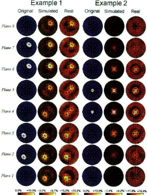
Figure 4. Comparison of simulated and real images. The original images, of change in conductivity Delta cn,

give a representation of nylon cylindrical blocks (diameter 50 mm, length 60 mm) positioned in a saline-filled (sigma = 4 mS cm sup -1) phantom. Example 1 corresponds to two blocks located at different heights and radial positions within the phantom. Example 2 corresponds to a single block positioned in the centre of the phantom. Simulated 3D images based on a 1,024 data set give a close representation of the original conductivity distribution with only limited Delta cn changes being

propagated into adjacent planes. Real images, reconstructed from data collected from the phantom, are less well defined but the nylon blocks can still be identified. METHODS. Simulated images are as described in figure 3. Real data were collected using a phantom with the same geometrical proportions as the 3D mesh offigure 2, using the Sheffield MK3b Electrical Impedance Tomographic

Spectroscope (EITS) (16). This 64-electrode system applies current at eight frequencies over the range 9.6 kHz to 1.2 MHz, and acquires a complete data set in 60 ms. A reference data set was collected from a saline-filled phantom with uniform conductivity. Nylon blocks were then submerged at positions represented by the simulated forward Delta cn image, and

another voltage measurement data set was collected. These are normalized to form the boundary data set Delta gn and reconstructed. Images are displayed with colour scales showing the maximum

values of percentage conductivity change.

Although the spatial resolution of 3D EIT (about 10% of image diameter in the cross-sectional plane and 12.5% in the axial plane) is worse than that of other imaging techniques such as magnetic resonance imaging and X-ray computed tomography, it does have several distinct advantages over existing medical imaging methods. These include safety, portability, long-term monitoring, cost, and the inherent ability to image physiological function. We are currently implementing a clinical trial to investigate the feasibility of using 3D EIT to detect pulmonary emboli. If the trial is successful, 3D EIT will provide an important alternative to the established radionuclide imaging technique.

ACKNOWLEDGEMENTS.

This work was supported by Action Research and EPSRC.

REFERENCES

1. Geddes, L. A. & Baker, L. E. Med. Biol. Engng 5, 271-293 (1967).

5. McAdams, E. T. & Jossinet, J. Physiol. Meas. A16, A1-A14 (1995). 6. Dawids, S. G. Clin. Phys. Physiol. Meas. A8, 175-180 (1987). 7. Dijkstra, A. M. et al. J. med. Engng Technol. 17, 89-98 (1993).

8. Holder, D. S. & Brown, B. H. in Clinical and Physiological Applications of Electrical Impedance Tomography (ed. Holder, D. S.) 47-60 (University College London Press, London, 1993). 9. Barber, D. C., Brown, B. H. & Freeston, I. L. Electron. Lett. 19, 933-935 (1983).

10. Barber, D. C. & Brown, B. H. J. Phys E: Sci. Instrum. 17, 723-733 (1984).

11. Barber, D. C. in Clinical and Physiological Applications of Electrical Impedance Tomography (ed. Holder, D. S.) 47-60 (University College London Press, London 1993).

12. Barber, D. C. & Brown, B. H. in Inverse Problems in Partial Differential Equations (eds. Colton, D., Ewing, R. Rundell, W.) 151-164 (Soc. for Industrial and Applied Mathematics, Philadelphia, 1990).

13. Rabbani, K. S. & Kabir, A. M. B. H. Clin. Phys. Physiol. Meas. 12, 393-402 (1991).

14. Morucci, J. P., Granie, M., Lei, M., Chabert, M. & Marsili, P. M. Physiol. Meas. A16, A123-A128 (1995). 15. Goble, J., Chenney, M. & Isaacson, D. Appl. Comput. Electromagn. Soc. J. 7, 128-147 (1992).

16. Brown, B. H. et al. (spec. iss. 1) Innov. Tech. Biol. Med. 15, 1-8 (1994). 17. Brown, B. H. & Seagar, A. D. Clin. Phys. Physiol. Meas. A8, 91-97 (1987). 18. Geselowitz, D. B. IEEE Trans. biomed. Engng 18, 38-41 (1971).

19. Kotre, C. J. Clin. Phys. Physiol. Meas. 10, 275-281 (1989). 20. Barber, D. C. Clin. Phys. Physiol. Meas. 10, 368-370 (1989). 21. Witsoe, D. A. & Kinnen, E. Med biol. Engng 5, 239-248 (1967).

22. Albert, A. Regression and the Moore-Penrose Pseudo-inverse (Academic, New York, 1972). 23. Golub, G. H. & Reinsch, C. Numer. Math. 14, 403-420 (1970).