The Effect of Rail Journey Time Improvements: Some Results and Lessons of British Experience Relevant to High Speed Rail Forecasting.

This is a repository copy of The Effect of Rail Journey Time Improvements: Some Results and Lessons of British Experience Relevant to High Speed Rail Forecasting..

White Rose Research Online URL for this paper: http://eprints.whiterose.ac.uk/2185/

Monograph:

Wardman, M. (1993) The Effect of Rail Journey Time Improvements: Some Results and Lessons of British Experience Relevant to High Speed Rail Forecasting. Working Paper. Institute of Transport Studies, University of Leeds , Leeds, UK.

Working Paper 388

eprints@whiterose.ac.uk https://eprints.whiterose.ac.uk/ Reuse

See Attached Takedown

If you consider content in White Rose Research Online to be in breach of UK law, please notify us by

White Rose Research Online

http://eprints.whiterose.ac.uk/

Institute of Transport Studies University of Leeds

This is an ITS Working Paper produced and published by the University of Leeds. ITS Working Papers are intended to provide information and encourage discussion on a topic in advance of formal publication. They represent only the views of the authors, and do not necessarily reflect the views or approval of the sponsors.

White Rose Repository URL for this paper: http://eprints.whiterose.ac.uk/2185/

Published paper

Wardman, M. (1993) The Effect of Rail Journey Time Improvements: Some Results and Lessons of British Experience Relevant to High Speed Rail

Forecasting. Institute of Transport Studies, University of Leeds. Working Paper 388

Working Paper 388

February

1993

THE EFFECT OF RAIL JOURNEY TIME

IMPROVEMENTS: SOME RESULTS AND

LESSONS OF BRITISH EXPERIENCE

RELEVANT TO HIGH SPEED RAIL

FORECASTING

M

Wardman

UNIVERSITY OF LEEDS

Institute for Transport Studies

ITS Working Paper 388

February 1993

THE EFFECT OF RAIL JOURNEY TIME

IMPROVEMENTS: SOME RESULTS AND LESSONS OF

BRITISH EXPERIENCE RELEVANT TO HIGH SPEED

RAIL FORECASTING

M Wardman

ITS Working Papers are intended to provide information and encourage discussion on a topic in advance of formal publication. They represent only the views of the authors, and do not

CONTENTS

Page

ABSTRACT

1.INTRODUCTION 1

2.OBJECTIVES 1

3.BACKGROUND: BRITISH FORECASTING PROCEDURE 2

4.AGGREGATE ECONOMETRIC MODELS 3

4.1Background 3

4.2Advantages of the method 4

4.3Drawbacks of the method 4

4.4Results from British experience 5

5.STATED PREFERENCE MODE CHOICE MODELS 10

5.1Background 10

5.2Advantages of stated preference 12

5.3Drawbacks of stated preference 12

5.4Results from British experience of stated preference 14

6.LESSONS FROM BRITISH EXPERIENCE 18

ABSTRACT

WARDMAN, M. (1993) The effect of rail journey time improvement: some results and lessons of British experience relevant to high speed rail forecasting. ITS Working Paper 388, Institute for Transport Studies, University of Leeds, Leeds.

This paper discusses the British experience of forecasting the effect of journey time reductions on the demand for rail travel. Its purpose is to discuss results and methodologies from the British context which may be appropriate to other contexts, and particularly to forecasting the demand for new high speed rail services. Two areas of research are selected for discussion: aggregate econometric models of rail demand and Stated Preference choice models. It is concluded that the results derived from one context may not be as transferable as one might wish to some other situation and that it is important to obtain a better understanding of the factors influencing journey time elasticities. Both of the demand analysis methodologies discussed could contribute to an improved understanding whilst an attraction of the Stated Preference approach is that it lessens the need to transfer results from one context to another.

KEY WORDS: Rail travel demand; journey time elasticities; high speed rail; stated preference.

THE EFFECT OF RAIL JOURNEY TIME IMPROVEMENTS: SOME

RESULTS AND LESSONS OF BRITISH EXPERIENCE RELEVANT TO

HIGH SPEED RAIL FORECASTING

1.

INTRODUCTION AND BACKGROUND

In the light of the new high speed rail service between Madrid and Seville, and with plans for other high speed rail services in Spain and continued strong interest in high speed rail elsewhere in Europe, the Spanish Railway Foundation and the Spanish Ministry of Transport organised a conference in Madrid on 2-3 December 1992 on the subject of the demand and regional effects of high speed rail. Researchers from Belgium, France, Italy, Germany, Great Britain and Spain presented evidence on the impact of high speed rail or of improvements to existing inter-urban rail services. This provided an insight into the various demand forecasting methodologies used in different contexts and into the experience of the actual impacts of those high speed services which have so far been introduced. This paper was presented at this conference and discusses evidence of the British experience of analysing the effects of gradual improvements in rail journey times.

Rail routes in Great Britain have generally been the subject of gradual improvements, with some lines upgraded to a maximum speed of 200 kph, short term possibilities to increase this to 225 kph, and longer terms plans for high speed rail links to the Channel Tunnel and substantial improvements to the West Coast Main Line (current maximum 175 kph) linking London with Birmingham, Manchester and Glasgow. Whilst there is no British experience of high speed rail operation, there is, however, a wealth of evidence and experience amassed over many years from numerous studies of the responsiveness of demand to variations in service quality and fares. Indeed, it is fair to say that the application of some methodologies to analyse travel demand (eg, stated preference) has been pioneered in the British context.

2. OBJECTIVES

The aims of this paper are:

i)to discuss results and methodologies from the British context which are appropriate for other contexts, and particularly high speed rail

ii)to highlight important lessons which have been learnt from British modelling experience

From amongst the large number of studies, using a variety of techniques and examining a wide range of issues, we have selected for discussion two areas of research which are most appropriate: a)Aggregate Econometric Models of Rail Demand

b)Stated Preference Choice Models.

This paper does not provide a comprehensive account of the application of these methods to inter-urban rail demand analysis in Britain. The reported studies have been selected to highlight the application of a particular methodology or, more importantly, because their results have implications for demand forecasting in the context of high speed rail. The paper focuses on improved rail services brought about by journey time reductions.

The current British Rail approach to forecasting journey time reductions employs a variable termed generalised time (GT) which represents the train quality of service aspects of journey time, interchange and frequency. It is calculated as:

INT i + FREQ p + JT =

GT (1)

where JT is station to station journey time, FREQ is the service frequency and INT denotes the number of interchanges required. The parameters p and i denote time penalties which convert the frequency and interchange terms into equivalent time units. The forecast of demand after some change in GT is simply calculated as:

V ) GT / GT ( =

V2 2 1 1

β

(2)

where 1 and 2 are the before and after time periods, V is the volume of rail demand and is the elasticity to GT. A value of -0.9 is used for . This value was taken from studies of high speed train introduction in Great Britain (OR, 1985b and see section 4 below) and has been substantiated in a number of subsequent studies. However, these studies generally used the constant elasticity form at the expense of allowing the elasticity to vary with relevant factors.

It can be shown that the elasticity to JT is not constant even though the elasticity to GT is. The relationship between the JT elasticity ( JT) and the GT elasticity ( GT) is:

η

η_{JT GT}

GT JT

= (3)

Thus if JT forms 90% of GT, the implied JT elasticity is -0.81, whereas it is only -0.45 if JT is 50% of GT. However, the elasticity variation which occurs within this forecasting procedure is simply the outcome of the formulation used and is not necessarily that which best explains actual behavioural responses. Moreover, the JT elasticity will be the same regardless of other relevant factors, such as the level of competition and the base level of JT, if the ratio of JT to GT is the same.

Constant elasticities are more appropriate for small changes in journey times associated with gradual improvements. Where larger changes are envisaged, in which case the limitations of the constant elasticity approach are recognised, specific studies are conducted, for example, for the Channel Tunnel (MVA 1988a) and plans to considerably upgrade the West Coast Main Line (MVA 1988b and see section 5)

Whilst the expense of such schemes justifies studies specific to the scheme, nonetheless the extent to which the results from TGV operation have been used to forecast other high speed rail schemes requires that a satisfactory understanding of the factors affecting demand and the journey time elasticity is obtained in order that the results can be confidently transferred to the particular circumstances of some other high speed rail project.

4. AGGREGATE

ECONOMETRIC

MODELS

4.1 BACKGROUND

Aggregate econometric models are based on measures of ticket sales, and are hence termed Revealed Preference methods since they are based on actual behaviour. They aim to explain variations in the volume of rail demand as a function of variations in relevant variables such as journey time, cost, the level of economic activity and, in some cases, generation and attraction factors. We are here concerned with models which aim to explain rail demand and not market share models of mode choice.

Fortunately, ticket sales data is available for a large number of station-to-station flows in Britain and it has supported a large amount of analysis over many years (eg, Evans, 1969; Fowkes et al., 1985; Jones and Nichols, 1983; OR, 1985b, 1989, 1991; Owen and Phillips, 1987; Tyler and Hassard, 1973; Wardman et al., 1992). The introduction of computerised ticket machines in the early and mid 1980's has meant that British Rail's ticket sales data is now regarded as providing a reliable account of the volume of travel between two points; it certainly compares very favourably with data sources which are used for other travel demand analysis purposes. The analysis can be based on:

i) pure time series data (One flow for many years) ii) pure cross-sectional data (Many flows for one year) iii) pooled time series and cross-sectional data.

The aggregate models which will be discussed here are based on pooled time series and cross-sectional data; more specifically, they are based on the analysis of changes in demand between two points in time across a large number of flows.

To illustrate the method, assume that rail demand is simply a function of rail generalised cost and that we can specify a simple demand function relating rail volume (V) and rail generalised cost (GCR) between any two points (i and j) in time period t as:

ijt GCR ijt k = ijt

V

β

where kijt represents the generating potential of origin i and the attracting potential of destination j in time period t. Expressing this as a ratio of demand in time periods 1 and 2 (for example, before and after a new high speed rail service) and assuming that the generation and attraction factors are constant over time, yields:

ij1 GCR

ij2 GCR =

ij1 V

ij2 V

β

β

(5)

which can be transformed for estimation of the unknown parameter by multiple regression:

ij1 GCR

ij2 GCR =

ij1 V

ij2 V

ln

ln

β

6 where ln denotes natural logarithm.

This basic model can be extended to include time trends, separate terms for the cost, time, frequency and interchange components of generalised cost, a range of other variables (eg, economic activity, competing modes) and also to allow generation and attraction factors to vary over time. More complicated functional forms can be used which, to varying extents, depart from the constant elasticity position.

4.2 ADVANTAGES OF THE METHOD

i) The method is relatively cheap and straightforward to undertake if measures of rail demand, fares and service quality are routinely collected and hence readily available.

ii) The method is regarded to provide a reliable indication of the effect of service characteristics and fare on demand since it is based on observations of actual changes. The degree of consistency between the results obtained from a number of applications in the British context is high.

iii) Examining changes in demand across a large number of routes is considered to avoid the worst excesses of simultaneity bias which is apparent in pure cross-sectional models. The latter have difficulty in distinguishing between whether, say, low frequency is the cause or consequence of low demand

iv) Since observations are taken across numerous routes, the data will exhibit more variation than a pure time series model. This increases the range of issues which can be examined and can contribute to more precise parameter estimates.

v) More data is obtained, able to support more detailed analysis and yielding more precise estimates, than if the data is a pure time series or cross-section.

4.3 DRAWBACKS OF THE METHOD

i) As with all aggregate methods, it is not possible to undertake certain disaggregated analysis of the data, for example, according to journey purpose or time of travel.

ii) It is limited to actual events. Clearly, high speed rail journey times cannot be examined if high speed rail does not exist.

iii) The data may suffer collinearity problems, whereupon there will be difficulties in discerning between the separate effects of correlated variables and the standard errors will be higher than otherwise. There may still also be problems of limited variation in some variables of interest (eg, car journey time changes over time).

7 accurately as possible.

4.4 RESULTS FROM BRITISH EXPERIENCE

We here present results from British experience of such (pooled time series and cross section) aggregate econometric models of rail travel demand which have examined the elasticity to journey time for inter-urban travel. We commence the discussion of the results of actual studies by reporting the main findings of a comparative analysis of the impact of the British high speed train (HST) and the French TGV Sud-Est. Analysis of the impact of these two rail services was undertaken by the Operational Research Division of British Rail (OR, 1985a, 1985b). Although the analysis was based on rather limited sample sizes, some interesting results emerged.

Data for before and after TGV Sud-Est introduction was supplied by SNCF for 26 Paris based flows and generalised speed (Q) measures consistent with those used by British Rail were calculated. The analysis of HST was based on 25 flows, 12 of which were London based. In the before year, the Q values were fairly similar on the two sets of flows. However, the post TGV values of Q were in the range 60-110 mph but the post HST values of Q had a range of somewhat lower speeds of 30-80 mph.

A range of models were estimated to the data. For the preferred constant elasticity model, the elasticity to Q for HST for London based flows was 0.91 but it was somewhat higher at 1.26 for the TGV flows. This higher elasticity for TGV could have arisen because:

i) TGV involved larger changes in Q;

ii)the French flows experienced much more competition from air than the British flows and hence there is a greater market from which rail can capture travellers;

iii)the journey distances were somewhat higher and the fares per distance somewhat lower for French flows.

Further analysis was undertaken of the French flows according to whether there was air competition or not. TGV flows which had no air competition were estimated to have elasticities of 1.17, still somewhat higher than for the HST flows. Although a model for TGV flows with airline competition was not reported, an elasticity of 1.37 would be consistent with the other TGV results.

Further evidence of TGV experience is consistent with the journey time elasticity varying with the size of the change in journey time and with the amount of air traffic to be captured. It is our understanding that after the opening of the first (Northern) section of TGV Sud-Est, the elasticity appeared to be 1.6 for a journey time reduction of around 30%, with an elasticity of not more than -1.1 for a journey time reduction of around 25% on the opening of the second (Southern) section. This was because the transfer from air had largely been completed in the first phase.

Care must always be taken in transferring or comparing results across different contexts, because there may be other relevant factors which have not been accounted for. However, these results do provide some evidence, admittedly of a tentative nature, to suggest that the degree of airline competition and the size of the journey time reduction affect the rail journey time elasticity.

More recent analysis using this method, which has focused on the impact of competition on rail demand and elasticities and on how rail elasticities with respect to some variable X might vary with the level of variable X, has been conducted at the Institute for Transport Studies (Wardman et al., 1992; Wardman 1992a).

For 119 observations of flows to and from London, the elasticity to (generally small) journey time changes estimated from a constant elasticity model was -0.66 with a rather large 95% confidence interval of ±85% of the central estimate. However, it was possible to obtain a statistically superior fit from a model possessing a journey time elasticity of:

D JT = JT β

η (7)

where D is distance. The journey time elasticity is proportional to the journey time per mile. Table 1 shows the implied point elasticities for a selection of flows in the data set.

Table 1: London time point elasticities

JT/D Elasticity

YORK-LONDON 0.71 -0.48

EDINBURGH-LONDON 0.76 -0.52

LEEDS-LONDON 0.81 -0.55

MANCHESTER-LONDON 0.88 -0.60

BIRMINGHAM-LONDON 0.92 -0.63

HULL-LONDON 1.05 -0.72

IPSWICH-LONDON 1.10 -0.75

NORWICH-LONDON 1.19 -0.81

ELY-LONDON 1.36 -0.93

As the journey time per mile increases, the journey time elasticity increases, and the variation across flows is quite considerable. There may be competitive effects at work here, but it is clear that the benefits of improving poorer services would be understated if the average journey time elasticity was used. We also tested a function which implied a larger elasticity for larger changes in journey time (JT). This could not provide an explanation which was as good as the constant elasticity model, but it is unlikely that the model could detect any effect which did exist because the journey time variations were low.

Although the 340 observations of Non-London flows in our data set are somewhat different in nature to flows upon which high speed rail services operate or are planned, the results for similar analysis of this data are illuminating. We have used a generalised time (GT) term for these flows,

since there were substantial combined improvements in time, frequency and interchange as a result of the introduction of many completely new cross-country services. The constant elasticity model produced an elasticity to GT of -0.99, which is similar to the value of -0.9 used by British Rail, and this had a relatively low confidence interval of ±16% of the central estimate. However, the model which best fit the data had an elasticity of:

D GT + GT =

GT β λ

η (8)

The GT elasticity varies with the absolute level of GT and the level of GT per mile (both and were negative). The implied elasticities for a selection of flows are given in Table 2.

Table 2: Non-London gt point elasticities

GT GT/D Elasticity

NORWICH-BIRMINGHAM 752 2.17 -1.58

LIVERPOOL-SHEFFIELD 488 3.32 -1.21

MANCHESTER-CARDIFF 756 2.23 -1.60

PORTSMOUTH-CARDIFF 574 2.11 -1.25

LEEDS-LIVERPOOL 345 2.34 -0.86

LEEDS-NEWCASTLE 372 1.76 -0.85

NEWCASTLE-IPSWICH 852 1.55 -1.71

SHEFFIELD-BIRMINGHAM 267 1.71 -0.66

BRADFORD-MANCHESTER 217 2.68 -0.65

Again, there is a considerable degree of variation in elasticities across routes and, if these elasticities provide a more reliable guide than the constant elasticity model, there may be significant errors in forecasting if the elasticity variation is ignored. The GT elasticity was also allowed to vary according to the size of the change in GT. This gave a fit as good as the constant elasticity model but not as good as equation 8.

Research is currently being undertaken at the Institute for Transport Studies on the effect of competition from car, air and coach on rail demand and elasticities for inter-urban travel. Very little is currently known in Britain about these effects. It is expected that rail elasticities and cross-elasticities of rail demand with respect to changes in the service characteristics and fares of competing modes will increase as rail market share falls. Some interesting results have so far emerged from our analysis.

In the first stage of our work, we examined the competition between rail, car and coach (it should be noted that there is a comprehensive network of deregulated coach services in Britain which provide competition to rail of varying strengths).

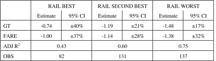
Generalised cost indices were calculated, using the data which had been collected on the service and cost characteristics of each mode, to provide measures of the relative attractiveness of the different modes. These measures are used since data on the market shares of each mode on each flow is not available. A data set of 350 flows were categorised according to whether rail was best (least generalised cost), worst (highest generalised cost) or second best (generalised cost lower than car or coach but not both). The elasticities, and 95% confidence intervals expressed as a proportion of the central estimate, are presented in Table 3. A strong relationship was found between rail elasticities, particularly that for GT, and the competitive position.

Table 3: Models segmented by relative generalised cost

RAIL BEST RAIL SECOND BEST RAIL WORST

Estimate 95% CI Estimate 95% CI Estimate 95% CI

GT -0.74 ±40% -1.19 ±21% -1.48 ±17%

FARE -1.00 ±37% -1.14 ±28% -1.38 ±32%

ADJ R2 0.43 0.60 0.75

OBS 82 131 137

More recently, we have examined the impact of airline competition on rail demand and elasticities. We were able to obtain plausible, and in some cases statistically significant, cross-elasticities of rail demand with respect to the time, frequency, interchange (which exists on some domestic UK air routes) and fare of air. More importantly, rail's own elasticities were found to vary with the degree of competition. However, due to the commercially confidential nature of the results, we are only able to quote orders of magnitude of the estimated effects. These are presented in Table 4 for flows where there was no air competition (NONE), weak air competition and strong air competition. The strength of competition is defined according to the level of accessibility to the air network. A distinction is made between London and Non-London flows because of possible different results due to the different mix of travellers (eg, business and leisure). A single category is used for weak competition since all but 26 of these were Non-London flows. The form of the estimated model is:

F F + e + A A + T T + P P + GT GT + = V V a1 a2 6 ) I -I ( a1 a2 4 a1 a2 3 1 2 2 1 2 1 0 1

2 _{5 a2 a1}

ln ln

ln ln

ln

ln β β β β β β β (9)

P denotes rail fare, and Ta, Aa, Ia and Fa denote the levels of travel (flight) time, adjustment time, interchange and fare for air. Ia denotes the number of interchanges involved and is specified in exponential form since it can be, and very often is, zero. However, some air services in Britain involve an interchange between two other services. Variations in Ia to some extent cause the variations in Ta although the statistical correlation between the two is not high. The adjustment time for air travel represents the difference between when travellers want to depart and can actually depart, weighted across a profile of desired actual departure times across the day. It therefore represents frequency effects.

11 Table 4: Elasticities and strength of airline competition

None Non-London None London Weak Strong Non-London Strong London GT X1 (±33%) X1+94% (±56%) X1+19% (±60%) X1+40% (±57%) X1+43% (±131%) FARE X2 (±32%) X2+21% (±67%) X2+43% (±40%) X2+159% (±23%) X2+157% (±53%)

TIME-AIR n/a n/a * X3

(±84%)

*

ADJ-AIR n/a n/a * X4

(±53%)

*

INT-AIR n/a n/a n/a X5 (±215%)

n/a

FARE-AIR n/a n/a * X6

(±155%)

*

OBS 529 127 199 171 84

ADJ R2 0.44 0.38 0.40 0.50 0.31

Notes: The figures in brackets denote 95% confidence intervals for the estimated coefficient. * denotes the 95% confidence interval exceeds ±250%. n/a denotes not applicable, either because there is no airline competition or else the variable exhibits zero variation.

All the GT and Fare elasticities, with the exception of the GT elasticity for London flows with strong air competition, are statistically significant. The London and Non-London flows with strong competition have similar own elasticities which are higher than for the flows with weak competition. In turn, with the exception of the GT elasticity for London flows with no air competition, the flows with weak competition have higher own elasticities than the flows with no air competition. It is not clear why the GT elasticity for London flows with no air competition is so high. The own-elasticities therefore exhibit the relationship with the degree of competition which we would hypothesise to exist.

These results are encouraging. However, the definition of competition used has an element of arbitrariness about it. In order to give the analysis a more objective basis, data was collected on the access times to and egress times from airports. This access and egress time, for a round trip, is termed accessibility (A). A large number of models were estimated which allowed the elasticities and cross-elasticities to vary according to the level of A. This was only done for Non-London flows because of the poor cross-elasticity results for London flows and the very limited variation in A on London flows.

In order to keep the analyis within manageable proportions, each variable was constrained to vary with A in the same manner (the combination of different functional forms and variables is very large). The model which was found to provide the best fit to the data was:

A = X

=

V β/ A η_X β

(10)

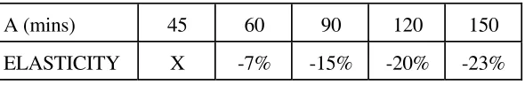
where X is any variable except Ia which was specified in exponential form to allow a similar effect from the level of A. This function implies that the elasticities fall as A increases, which is consistent with our theoretical expectations, and that the rate at which they fall diminishes. The variation is the same for all the elasticities and is depicted in Table 5 for a range of A which cover the levels of A which existed in the data set.

The degree of elasticity variation, and the absolute elasticities which were obtained, appear very plausible. The research is continuing, and will extend the definition of the competition variable to include whether rail allows a round trip to be made in a day, relative door-to-door journey time and relative generalised cost. In addition, further data has been collected with which to assess the effect of competition from car and coach.

Table 5: Elasticities and accessibility

A (mins) 45 60 90 120 150

ELASTICITY X -7% -15% -20% -23%

5.

STATED PREFERENCE MODE CHOICE MODELS

5.1 BACKGROUND

An alternative estimation and forecasting methodology is provided by what is termed the Stated Preference approach. Its most common application has been to mode choice, although it has also been applied in other contexts such as route choice, destination choice, departure time (eg, train service) choice and frequency of travel choice.

In practice, individuals choose between modes, say rail and air, on the basis of relevant variables such as journey time, cost, frequency, interchange and access/egress time. Revealed Preference mode choice modelling collects information on these characteristics and on the choices made by

individuals. It develops statistical models to explain the relationships between relevant variables and choice and hence is in a position to forecast the effect on choice of some change to travel circumstances, such as the introduction of a high speed rail service. The most commonly used model is the logit model which, for the choice between n alternatives, takes the form:

e e = P _U n U 1 n 1

∑ (11)

where P1 is the probability of choosing or the market share of mode 1. The utility associated with any mode i (Ui) is related to the k observable variables which influence choice:

) X , ( f =

Ui

α

The unobserved elements of choice enter the error term which in turn influences the absolute values of the estimates of the ik. It is the assumptions regarding the form of the error term which determine the particular model which is derived. Assuming the errors associated with each alternative to be independently and identically distributed and to follow a type I extreme value distribution yields the familiar logit model. At least in the British context, such models are disaggregate, that is, they are based on individuals' discrete (0-1) choices, rather than on market share information, and the model is estimated using maximum likelihood. Fowkes and Nash (1991) provide further details of the method in the context of rail demand.

The method of Stated Preference differs from that of Revealed Preference only in terms of the form of the data which is used to develop the model. The latter is based on actual choices and actual travel characteristics which exist in the market place. Stated Preference instead offers individuals a series of hypothetical travel scenarios to be evaluated. Thus we would obtain data on a number (typically between 9 and 16) of choices between, say, rail and air, each with specific travel characteristics. Models are developed to explain these choices in an entirely analagous fashion to Revealed Preference data. Whilst the levels of the travel variables for each mode and across each comparison are specified to have the features required by the analyst (eg, zero correlations between variables, high speed rail travel times), they must nevertheless be plausible and exhibit required relationships between modes if individuals are to provide sensible answers.

There are a number of issues relating to the design of Stated Preference experiments and to data collection. We shall not discuss these here but the interested reader is referred to a special edition of the Journal of Transport Economics and Policy (January 1988) which covers a whole range of issues related to the use of Stated Preference methods in transport.

The method has been widely used in Britain, both for urban and inter-urban travel, and has been applied to all modes of transport, although particularly to rail. In the case of inter-urban rail travel, it has been used to forecast choices between rail and air for business travellers (Steer Davies Gleave et al., 1989; Wardman, 1992b), between rail, coach and car for leisure travellers (TPA, 1992; TSU, 1989) and for studies related to the Channel Tunnel (Euromap, 1989; Harris et al. 1990). It has been widely used to value rail attributes. Examples include the valuation of interchange (MVA, 1985), departure time variations (Wardman and Fowkes, 1987), crowding (MVA et al., 1989a; Wardman and Fowkes, 1987), station facilities (MVA, 1988c), reliability and frequency (Steer Davies Gleave, 1981; MVA et al., 1989b), and stock type and on-train facilities (MVA, 1986). Stated Preference has been widely used for these variables because of the limitations of Revealed Preference methods in these areas, but more reliance is placed on Revealed Preference evidence for price elasticity

14

effects, and particularly variables such as car ownership and economic activity which Stated Preference is not well suited to examine.

5.2 ADVANTAGES OF STATED PREFERENCE

Stated Preference is of use where a mode does not exist and hence where Revealed Preference models cannot be developed. High speed rail may fit into this category. Whilst revealed preference mode choice models can be based on, for example, the choices between conventional train, car, air and coach, they cannot model the response to the low journey times offered by high speed rail. More data is collected since individuals make multiple choices between alternatives rather than the single observation of Revealed Preference. Data collection is therefore cheaper for a given level of precision or the estimates are more precise for a given number of individuals contacted.

Revealed Preference data may be deficient in several respects. It may contain large correlations between variables or else some variables of interest may exhibit insufficient variation. In contrast, Stated Preference experiments can largely control, within the bounds of realism, the level of correlation and variation.

Unlike methods based on ticket sales data, Stated Preference is essentially a disaggregate approach. It therefore allows more disaggregated analysis, such as examining how relative values (eg, the value of time), elasticities and demand forecasts vary according to socio-economic factors such as journey purpose, income level, age, sex and social class.

5.3 DRAWBACKS OF STATED PREFERENCE

The main advantages of Stated Preference stem from an ability to control the independent variables. In contrast, Revealed Preference methods are based on what people do, rather than what they say they will do, and the main criticisms of Stated Preference relate to its dependent variable, that is there are concerns as to the reliability of the choices stated by individuals.

The responses supplied by individuals may not accurately reflect what they would do in particular circumstances. There may be error of a random nature, such as that arising from misunderstanding, response fatigue or an uncertainty as to which mode is preferred. What is more serious is systematic error or bias in responses. The literature identifies several forms of bias which may affect Stated Preference responses (Mitchell and Carson, 1989; Wardman, 1991). In addition, the coefficient estimates of discrete choice models are scaled relative to the residual deviation, and error which enters Stated Preference responses but which would not affect actual choices is allowed to influence the coefficients and hence forecasts. This is termed the scale factor problem (Bates, 1988). However, evidence on the degree of correspondence between valuations and forecasts derived from Stated and Revealed Preference methods is encouraging (Fowkes, 1992; Wardman, 1988, 1991), whilst rescaling is possible relative to data on revealed preferences or by reference to some 'known' elasticity.

15

5.4 RESULTS FROM BRITISH EXPERIENCE OF STATED PREFERENCE

We will discuss some results from relevant Stated Preference studies which have examined the impact of rail travel time savings in the context of inter-urban travel.

In July 1991, electrification of the East Coast Main Line reduced the journey time between Edinburgh and London from around 4 hours 30 minutes to 4 hours. In March 1991, we undertook a Stated Preference experiment in order to forecast the response of business travellers from Edinburgh to London to the journey time reduction (Wardman, 1992b). In addition, we examined their responses to hypothetical journey times of 3 hours 40 minutes and 3 hours 20 minutes. The latter would imply an average speed of 190kph.

The Stated Preference experiment offered each business traveller 12 choices between the following options:

i) Air iv) Sleeper First Class

ii) Rail First Class v) Sleeper Standard Class iii) Rail Standard Class

The variables used to define each option were:

i) Access/Egress Time (All Options) iii) Cost (All Options) ii) Travel Time (Daytime Rail Only) iv) Idle Time (Sleeper Only)

In addition, half of the questionnaires specified a Pullman service in first class. Air flight time and sleeper time were both held constant at their current levels since it was considered unrealistic to vary them and indeed there was no need to do so. However, the implied level of idle time involved in using the sleeper, defined as the difference between the time of the meeting and the time of having to depart the Sleeper berth minus the egress time, entered the estimated model.

Responses were obtained from 53 business travellers with 550 usable observations for modelling. A multinomial logit model was developed, since the results from a hierarchical logit model showed the latter to be equivalent to the former (logsum parameter close to 1). Statistically significant values were obtained for journey time, access/egress time and idle time, although they were similar and insignificantly different and hence a single combined time term was used instead.

Table 6: Actual (sample) market shares

AIR DAY 1ST DAY STD SLEEPER 1ST SLEEPER STD

80% 7% 3% 8% 2%

The information on each individual's reported times and costs for rail and air were entered into the logit model estimated on the Stated Preference data. This produces for each individual a probability of choosing each option and the aggregate market shares are estimated as the weighted sum of individuals' choice probabilities. The estimated market share are reported in Table 7.

Table 7: Market shares predicted by SP model

AIR DAY 1ST DAY STD SLEEPER 1ST SLEEPER STD

77% 6% 3% 11% 3%

The SP market shares correspond very closely with the actual market shares. This is encouraging with respect to the validity of using the model to forecast changes in rail market share as a result of journey time reductions.

The incremental form of the logit model was used to forecast. This model takes the form:

e P

e P =

S _U

n n

U 1 1

n 1

∆ ∆

∑

where S1 is the market share of alternative 1 after the change, Pn is the market share for alternative n in the before situation, and Un is the change in the utility of alternative n between the two situations. Since we are only interested in changes in journey time, the utility difference can be simply calculated as the product of the time difference and the time coefficient. The only other input required is the base market share of each alternative and for this purpose we have used the market share estimates based on the actual choices of our sample (Table 6). We have forecast the revised market shares for each option for daytime rail journey times of 4 hours, 3 hours 40 minutes and 3 hours 20 minutes, all other variables remaining unaltered. These journey times are in relation to the base of the current 4 hours 30 minutes. The forecasts are given in Table 8.

The rail journey time reductions do not greatly alter air's dominance in the market but do lead to large proportionate increases from the low base daytime train demand. However, this gain is offset by switching from the more expensive sleeper alternatives to daytime train.

Table 8: Forecasts for rail journey time reductions

Air Day 1st Day Std Sleeper 1st Sleeper Std

Base 80.0% 7.0% 3.0% 8.0% 2.0%

4 Hours 77.3% 9.2% 3.9% 7.7% 1.9%

3 Hours 40 75.0% 10.9% 4.7% 7.5% 1.9%

3 Hours 20 72.5% 12.9% 5.5% 7.3% 1.8%

The elasticities implied by a logit model will, amongst other things, depend on the market share of rail. The logit model's point elasticity of rail demand with respect to rail journey time is:

) P -(1 JT

= r r

point

α

η

where is the time coefficient, JTr is the journey time of rail and Pr is the probability of choosing rail. However, we are not concerned here with marginal changes in journey time and hence the journey time elasticities have been calculated on the basis of the arc-elasticity defined as:

. JT -JT V -V = 1 2 1 2 ln ln ln ln arc

η (15)

The arc-elasticities implied are given in Table 9, and reflect the proportionate changes in rail volume from the base situation, including the Sleeper market share in the overall measure of rail demand.

Table 9: Journey time elasticities

JT % JT Elasticity

4hrs 30m - 4hrs 00m -11% -1.08

4hrs 30m - 3hrs 40m -19% -1.08

4hrs 30m - 3hrs 20m -26% -1.06

There is no need to allow for generation since this is expected to be negligible for business travel. These journey time elasticities are higher than are used in practical forecasting. This may be due to the sample being solely of business travellers or distance effects, although we are unable to determine the relative effect of each. However, they are lower than the elasticities which appear to be used for high speed rail project forecasts in Europe, even though the elasticities here relate only to business travellers.

A study was undertaken in 1988 (Steer Davies Gleave et al, 1989) which was primarily concerned with the price elasticity of demand of business travellers but which also estimated journey time elasticities. A Stated Preference experiment was presented to business travellers by train offering them a series of choices between rail and the reported best alternative mode. The modes were

18

described in terms of travel time and cost. The choices open to respondents were first class rail, full fare standard class rail, discount standard class rail, best competing mode and not travel.

Four hundred and thirty seven business travellers were interviewed, spread fairly evenly between the following five routes with the associated strength of competition from other modes.

i) Swindon-London Strong Competition (Car) ii) Cardiff-London Weak Competition

iii) Manchester-London Strong Competition (Air and Car) iv) Newcastle-London Medium Competition (Air) v) Edinburgh-London Very Strong Competition (Air)

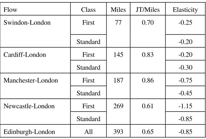
The interviews confirmed that the car was strongly favoured for shorter distance journeys but was considered inappropriate for longer distance journeys where air became the main competitor to rail. The journey time elasticities obtained, for 20% increases in journey time, are given for each class of travel in Table 10.

The elasticities, in general, are somewhat less than recommended values, even for relatively large changes in journey time but, as might be expected, they tend to be higher for first class travellers. Although Swindon has a low elasticity despite strong competition from car, it may be that it is difficult for rail to attract from car on such short distance journeys.

Whilst there seems to be a tendency for the elasticity to be higher where there is stronger competition, there also seems to be a distance related effect which appears to be larger than that estimated by the aggregate model reported in Table 1. The Edinburgh elasticity is not directly comparable with those in Table 9 since it relates only to sleeper travel. However, the London to Newcastle flow, which involves the next longest distance and experiences quite strong airline competition, has elasticities in line with those of Table 9.

Table 10: Business travel time elasticities

Flow Class Miles JT/Miles Elasticity

Swindon-London First 77 0.70 -0.25

Standard -0.20

Cardiff-London First 145 0.83 -0.20

Standard -0.30

Manchester-London First 187 0.86 -0.75

Standard -0.45

Newcastle-London First 269 0.61 -1.15

Standard -0.85

19

Finally, we discuss the results of research (MVA, 1988b) which was commissioned in the light of plans to upgrade the West Coast Main Line between London and Manchester and London and Birmingham to provide substantial time savings (around 40% on the former route and 25% on the latter). Again a Stated Preference experiment was used, because there are no actual cases of substantial improvements in journey time which could be monitored. It involved two components, one relating to mode switching behaviour and the other relating to the frequency of trip making and hence including generation effects.

The mode choice Stated Preference experiment involved trade-offs between journey time, fare, frequency of service and punctuality, the latter defined in terms of the late arrival time of one in ten trains. The frequency exercise was based on journey time, fare and punctuality. The journey times presented varied from current levels to levels consistent with 300kph operation. The study involved both business and leisure travellers.

Forecasts were obtained for 10%, 25% and 35% journey time reductions, with the reported values being central estimates. The journey time elasticities are given in Table 11. Again the elasticities are higher for first class travellers. In general, however, these journey time elasticities are low. Indeed they are not only lower than those relating to TGV, but the estimates for the Manchester flow are lower than current British conventions. There are two reasons why they might be underestimates.

i)Frequency change Stated Preference experiments are more difficult than those for mode choice. Respondents may not fully appreciate the increased journey opportunities facilitated by high speed rail

ii) Generation of totally new trips was not asked of those who undertook the mode choice experiment.

However, there are arguments which would suggest that the journey time elasticities derived from such an exercise could be too high. Bias which operates to overstate usage in response to journey time reductions, either because of an overenthusiasm about the scheme or else deliberately distorted answers which aim to increase the chances that the scheme is implemented, would both lead to higher elasticities. Thus it is by no means certain that the elasticities derived are underestimates, particularly since point ii) is unlikely to have led to a large underestimate of usage.

Table 11: High speed elasticities

ROUTE TICKET TYPE ELASTICITY

Manchester First -0.57

Full Standard -0.40

Discount Standard -0.31

Birmingham First -1.56

20

Discount Standard -0.48

6.

LESSONS FROM BRITISH EXPERIENCE

Although there is no British experience of operating rail services in excess of 200kph, the analysis of improvements to existing services using measures of changes in ticket sales and of hypothetical journey time improvements using Stated Preference data provide some interesting results.

i)The results derived from one context (eg, TGV introduction) may not be as transferable as we might wish to some other context. The British experience from a number of studies, using both Revealed and Statetd Preference data and including studies which have examined speeds consistent with high speed rail operation, is that journey time elasticities are somewhat lower than appear to be used (around -1.3) in high speed rail project appraisal in Europe.

ii)It is therefore important to obtain an understanding of the factors influencing the journey time elasticity. For example, we have reported in this paper results which show the time elasticity to vary according to the journey time per unit of distance and according to the level of competition from air, car and coach, as well as according to class of travel.

iii)The method of Stated Preference could contribute to an understanding of the journey time elasticities which are applicable to a particular context. Its importance relates to its ability to examine services such as high speed rail which might not yet exist and to account for the competitive environments in which rail journey time improvements are made. This ability to examine high speed rail on a particular route reduces the need to be able to transfer results from one context to another.

7.

REFERENCES

BATES, J.J. (1988). Econometric issues in stated preference analysis. Journal of Transport Economics and Policy22, pp.59-69.

BONNAFOUS, A. (1987). The regional impact of the TGV. Transportation18, pp. 127-137.

EUROMAP (1989). Business travel on the cross channel route. Prepared for SNCF, BR, SNCB and DB. Unpublished.

EVANS, A. (1969). InterCity travel and the LM electrification. Journal of Transport Economics and Policy.

FOWKES, A.S. (1992). How reliable is stated preference. Working Paper 377, Institute for Transport Studies, University of Leeds

21

FOWKES, A.S., Nash, C.A. and Whiteing, A.E. (1985). Understanding trends in intercity rail traffic in Great Britain. Transport Planning and Technology, 10 pp. 65-80.

HARRIS RESEARCH, ACCENT RESEARCH and HAGUE CONSULTING GROUP (1990). Channel Tunnel leisure study. Prepared for BR, DB, NS, SNCB and SNCF.

JONES, I. and NICHOLS, A. (1983). Demand for Inter-City rail travel. Journal of Transport Economics and Policy.

MITCHELL, R.C. and CARSON, R.T. (1989). Using surveys to value public goods: the contingent valuation method. Resources for the Future, Washington DC.

MVA CONSULTANCY (1985). Interchange. Prepared for British Railways Board, Unpublished.

MVA CONSULTANCY (1986). Evaluation of intercity rolling stock improvements. Prepared for InterCity, British Railways Board, Unpublished.

MVA CONSULTANCY (1988a). Channel Tunnel forecasts. Prepared for BRB, Unpublished.

MVA CONSULTANCY (1988b). West coast main line: market research. Prepared for InterCity, British Railways Board, Unpublished.

MVA CONSULTANCY (1988c). Station modernisation priorities and pay-offs. Prepared for British Railways Board, Unpublished.

MVA CONSULTANCY and INSTITUTE FOR TRANSPORT STUDIES, UNIVERSITY OF LEEDS (1989a). Provincial overcrowding study. Prepared for Provincial Railways, Unpublished.

MVA CONSULTANCY and INSTITUTE FOR TRANSPORT STUDIES, UNIVERSITY OF LEEDS (1989b). Network SouthEast quality of service study. Prepared for Network SouthEast, British Railways Board, Unpublished.

OR - OPERATIONAL RESEARCH DIVISION, BRITISH RAIL (1985a). Analysis of TGV service elasticities. Memo 10102/M1

OR - OPERATIONAL RESEARCH DIVISION, BRITISH RAIL (1985b). Further analysis of HST and TGV Results. Memo 10102/M2

OR - OPERATIONAL RESEARCH DIVISION, BRITISH RAIL (1989). Estimation of the elasticity to changes in fare. Memo 10329/M2, Unpublished.

OR - OPERATIONAL RESEARCH DIVISION, BRITISH RAIL (1991). Sprinter introduction on the Midland express. Memo 10344/M1, Unpublished

OWEN, A. and PHILLIPS, G.D. (1987). The characteristics of railway passenger demand. Journal of Transport Economics and Policy.

22

STEER DAVIES GLEAVE, HAGUE CONSULTING GROUP, ACCENT RESEARCH (1989). InterCity business travel price elasticity research. Prepared for InterCity, Unpublished.

TPA CONSULTANCY (1992). TransPennine rail study. Warrington, UK. Unpublished.

TSU - TRANSPORT STUDIES UNIT, UNIVERSITY OF OXFORD (1989). Rail price elasticities in the long distance leisure market. Prepared for InterCity, British Railways Board.

TYLER, J. and HASSARD, R. (1973). Gravity/elasticity models for the planning of the inter urban rail passenger business" PTRC Summer Annual Meeting.

WARDMAN, M. (1988). A comparison of revealed preference and stated preference models of travel behaviour" Journal of Transport Economics and Policy22, pp.71-91.

WARDMAN, M. (1991). Stated preference methods and travel demand forecasting: an examination of the scale factor problem. Transportation Research25A, pp.79-89.

WARDMAN, M. (1992a). Competitive modelling study: analysis of outliers, stock type and functional form. Technical Note 299, Institute for Transport Studies, University of Leeds.

WARDMAN, M. (1992b). An analysis of the mode choice behaviour of business travellers between Edinburgh and London. Technical Note 304, Institute for Transport Studies, University of Leeds.

WARDMAN, M. and FOWKES, A.S. (1987). The values of overcrowding and departure time variations for InterCity rail travellers. Technical Note 229, Institute for Transport Studies, University of Leeds.

WARDMAN, M., BRISTOW, A. and FOWKES, A.S. (1992). Competitive modelling of inter-urban rail demand" Technical Note 300, Institute for Transport Studies, University of Leeds.