Baryon and lepton numbers in particle physics
beyond the standard model
Thesis by
Jonathan M. Arnold
In Partial Fulfillment of the Requirements for the Degree of
Doctor of Philosophy
California Institute of Technology Pasadena, California
2014
Abstract
The works presented in this thesis explore a variety of extensions of the standard model of particle physics which are motivated by baryon number (B) and lepton number (L), or some combination thereof. In the standard model, both baryon number and lepton number are accidental global symmetries violated only by non-perturbative weak effects, though the combinationB −Lis exactly conserved. Although there is currently no evidence for considering these symmetries as fundamental, there are strong phenomenological bounds restricting the existence of new physics violatingBorL. In particular, there are strict limits on the lifetime of the proton whose decay would violate baryon number by one unit and lepton number by an odd number of units.
The first paper in this thesis explores some of the simplest possible extensions of the standard model in which baryon number is violated, but the proton does not decay as a result. The second paper extends this analysis to explore models in which baryon number is conserved, but lepton flavor violation is present. Special attention is given to the processes of µ to e conversion and µ → eγ which are bound by existing experimental limits and relevant to future experiments.
Contents
Acknowledgments iv
Abstract v
1 Introduction 1
2 Simplified models with baryon number violation but no proton decay 6
2.1 Introduction . . . 6
2.2 The models . . . 8
2.3 Phenomenology of model 1 . . . 15
2.3.1 Neutron-antineutron oscillations . . . 15
2.3.2 LHC, flavor and electric dipole moment constraints . . . 18
2.3.3 Baryon asymmetry . . . 20
2.4 Conclusions . . . 22
Appendices 24 2.A Vacuum insertion approximation . . . 24
2.B Down quark edm . . . 25
2.C K0-K¯0mixing . . . 28
2.D Absoptive part ofX2 decay . . . 29
3.2 Models . . . 33
3.3 Phenomenology . . . 35
3.3.1 Naturalness . . . 35
3.3.2 µ→eγ decay . . . 36
3.3.3 µ→econversion . . . 38
3.3.4 Electron EDM . . . 43
3.4 Baryon number violation and dimension five operators . . . 45
3.5 Conclusions . . . 47
Appendices 49 3.A Calculation ofµ→eγ . . . 49
4 Supersymmetric Dark Matter Sectors 53 4.1 Introduction . . . 53
4.2 Supersymmetric Dark Sector . . . 55
4.3 Dark Matter Relic Density . . . 59
4.4 Predictions for DM Direct Detection . . . 62
4.5 Conclusions . . . 65
5 B and L at the SUSY Scale, Dark Matter and R-parity Violation 67 5.1 Introduction . . . 67
5.2 Spontaneous Breaking ofB andL . . . 69
5.2.1 Symmetry Breaking and Gauge Boson Masses . . . 71
5.2.2 Spontaneous R-parity Violation . . . 74
5.3 Dark Matter Candidates . . . 75
5.4 Conclusions . . . 79
Chapter 1
Introduction
the standard model, and both are observed to be extremely good symmetries of nature. The proton, for example, is known to have a lifetime of at least∼ 1034years. However, there is no fundamental symmetry guaranteeing its absolute stability in the same way that, for example, electromagnetic gauge invariance guarantees the stability of the electron. In fact, it is known that both baryon and lepton numbers are violated by non-perturbative weak pro-cesses. This is due to the fact that, in the standard model, each of these global symmetries is anomalous. That is, they are classical symmetries of the standard model, but each is broken by non-perturbative quantum effects. Although these effects are small enough to be negli-gible in laboratory experiments, they can be important in studying the early universe when temperatures were much higher. Indeed, the standard modern cosmological models rely on a violation of baryon number to explain the matter asymmetry observed in the universe – a violation ofB is one of the three Sakharov conditions necessary for baryogenesis. A violation of lepton number is another popular ingredient in early universe cosmology since a lepton asymmetry can generate a baryon asymmetry viaB- andL-violating sphalerons – a mechanism known as leptogenesis. In any case, there is a tension between the apparent necessity for baryon and lepton number violation in models of early universe cosmology and the strict bounds placed on the violation of these symmetries generated by laboratory experiments. It is this tension, in part, which has motivated the works included in this thesis.
strongly constrained by both flavor physics and limits on the electric dipole moment of the neutron. We explore the parameter space of one model in particular to show that it can be in agreement with current experimental bounds, but still have measurable effects in the next generation of neutron oscillation experiments.
In Chapter 3, we use a very similar approach to model building, this time with the goal of exploring simple extensions of the standard model which include lepton flavor violation. In this case, models with (perturbative) baryon number violation in the Yukawa sector are ignored, and only models with a single additional scalar field are considered. Only two such models exist, one of which is characterized by an unusual enhancement to the lepton flavor violating processµ→ eγ proportional to the top quark mass. The phenomenology of this model is investigated in detail, including a careful calculation of theµ → eγ decay rate, theµ→econversion rate, and the constraints coming from the electric dipole moment of the electron. We find that the model could have measurable effects in the charged lepton sector which would be observed at the MEG experiment (µ → eγ) and at the prospective Mu2e experiment (µ→e).
The last two chapters of this thesis were motivated by the second half of the tension mentioned earlier – the strict limits on the structure of new physics coming from mea-sured bounds on baryon and lepton number violating processes in laboratory experiments. These works focus on the possibility that these symmetries are not simply accidental global symmetries of the low energy theory, but rather relics of some more fundamental sponta-neously broken symmetry related to these numbers. In addition, the models are built into the minimal supersymmetric standard model (MSSM) in part because of the new gauge symmetries’ ability to replace R-parity, usually included in the MSSM to avoid dangerous
B- andL-violating terms in the superpotential.
Chapter 4 develops an extension of the MSSM which includes a spontaneously broken
introducingB−Las a spontaneously broken gauge symmetry is that it eliminates the need for an ad-hoc R-parity, usually introduced to explain away the existence of baryon and lepton number violating terms in the MSSM superpotential. In the model we introduce in Chapter 4, the MSSM is endowed with an extended gauge sector includingU(1)B−L. The
gauge symmetry is broken by the vacuum expectation value of the right-handed sneutrino, which then communicates this breaking via the D-term to a dark sector charged under
B−L. This process breaks supersymmetry in the dark sector and introduces a mass splitting among the new fields. The lightest of these particles is a good dark matter candidate. One interesting feature of this model is that, although R-parity is broken in the visible sector, no discrete symmetry is needed to guarantee the stability of the dark matter candidate. We show that the dark matter in this model is capable of reproducing the measured thermal relic abundance while still escaping the experimental bounds set by Xenon100.
In Chapter 5, we take a similar approach to extending the MSSM, this time by intro-ducing an extended gauge sector includingU(1)B⊗U(1)L. This gauge group has the
ad-vantage of eliminating non-renormalizable terms in the superpotential likeQˆQˆQˆL/ˆ Λand ˆ
ucuˆcdˆceˆc/Λ. These terms, which appear for example inSU(5)extensions of the MSSM, do
not violate either R-parity orB−L. However, bounds on proton decay limit the scaleΛto be greater than1027GeV – an enormous suppression that warrants theoretical grounding. Because these terms violateBandLseparately, gauging these symmetries provides a sim-ple possible mechanism for explaining this suppression. However, in the MSSM, U(1)B
and U(1)L are anomalous symmetries and so cannot be gauged without introducing new
particle content to cancel anomalies in this new gauge sector. In this chapter, we introduce a set of superfields we call leptoquarks with bothB andLquantum numbers that do just that, as well as the minimal new field content necessary to spontaneously break these local symmetries. We find that the breaking scale of U(1)B ⊗U(1)L and supersymmetry are
Chapter 2
Simplified models with baryon number
violation but no proton decay
2.1
Introduction
The standard model has non-perturbative violation of baryon number (B). This source of baryon number non-conservation also violates lepton number (L), however, it conserves baryon number minus lepton number (B −L). The violation of baryon number by non-perturbative weak interactions is important at high temperatures in the early universe, but it has negligible impact on laboratory experiments that search for baryon number viola-tion and we neglect it in this paper. If we add massive right-handed neutrinos that have a Majorana mass term and Yukawa couple to the standard model left-handed neutrinos, then lepton number is violated by two units,|∆L|= 2, at tree-level in the standard model.
Motivated by Grand Unified Theories (GUT) there has been an ongoing search for proton decay (and bound neutron decay). The limits on possible decay modes are very strong. For example, the lower limit on the partial mean lifetime for the modep→e+π0is 8.2×1033yrs[46]. All proton decays violate baryon number by one unit and lepton number by an odd number of units. See Ref. [71] for a review of proton decay in extensions of the standard model.
and discussing some of their phenomenology. We include all renormalizable interactions allowed by theSU(3)×SU(2)×U(1) gauge symmetry. In addition to standard model fields these models have scalar fields X1,2 that couple to quark bilinear terms or lepton bilinear terms. Baryon number violation either occurs through trilinear scalar interactions of the type (i) X2X1X1 or quartic scalar terms of the type (ii) X2X1X1X1. The cubic scalar interaction in (i) is similar in structure to renormalizable terms in the superpotential that give rise to baryon number violation in supersymmetric extensions of the standard model. However, in our case the operator is dimension three and is in the scalar potential. Assuming no right-handed neutrinos there are four models of type (i) where each of the
X’s couples to quark bilinears and has baryon number−2/3. Hence in this case theX’s are either color3 or¯6. There are also five models of type (ii) whereX1 is a color3 or¯6 with baryon number −2/3that couples to quark bilinears and X2 is a color singlet with lepton number−2that couples to lepton bilinears.
We analyze one of the models in more detail. In that model theSU(3)×SU(2)×U(1) quantum numbers of the new colored scalars areX1 = (¯6,1,−1/3)andX2 = (¯6,1,2/3). The nn¯ oscillation frequency is calculated using the vacuum insertion approximation for the required hadronic matrix element and lattice QCD results. For dimensionless coupling constants equal to unity and all mass parameters equal, the present absence of observednn¯ oscillations provides a lower limit on the scalar masses of around500 TeV. If we consider the limitM1 M2then forM1 = 5 TeVthe next generation ofnn¯oscillation experiments will be sensitive toM2masses at the GUT scale.
There are three models that havenn¯mixing at tree-level without proton decay. In these models, constraints on flavor changing neutral currents and the electric dipole moment (edm) of the neutron require some very small dimensionless couplings constants if we are to have both observablenn¯oscillations and one of the scalar masses approaching the GUT scale.
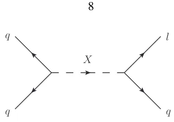
X q
q
l
[image:14.612.216.388.69.190.2]q
Figure 2.1:∆B = 1and∆L= 1scalar exchange.
d e
X
u
c s
W
e
ν
Figure 2.2: Feynman diagram that contributes to tree-level p → K+e+e−ν¯ from
(3,1,−4/3)scalar exchange.
concluding remarks are given in Section 2.4.
2.2
The models
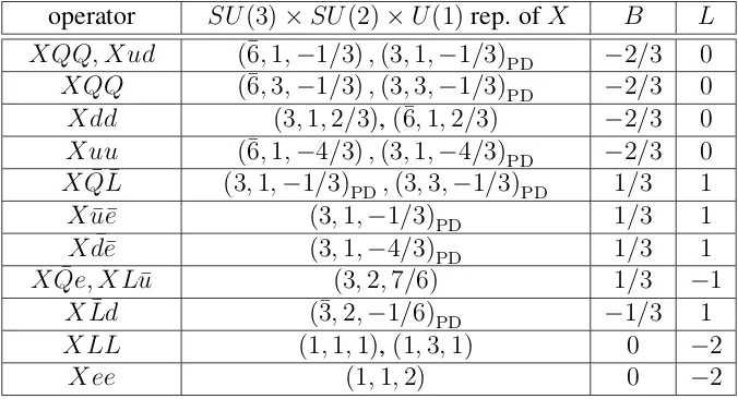
[image:14.612.225.381.248.346.2]ex-change to get proton decay (Fig. 2.2) since the Yukawa coupling to right-handed charge 2/3 quarks is antisymmetric (for a detailed discussion see [6]). The remaining possible scalar representations and Yukawa couplings are listed in Table 2.1. We have assumed there are no right-handed neutrinos (νR) in the theory.
operator SU(3)×SU(2)×U(1)rep. ofX B L XQQ, Xud (¯6,1,−1/3),(3,1,−1/3)PD −2/3 0
XQQ (¯6,3,−1/3),(3,3,−1/3)PD −2/3 0
Xdd (3,1,2/3),(¯6,1,2/3) −2/3 0
Xuu (¯6,1,−4/3),(3,1,−4/3)PD −2/3 0
XQ¯L¯ (3,1,−1/3)PD,(3,3,−1/3)PD 1/3 1
Xu¯e¯ (3,1,−1/3)PD 1/3 1
Xd¯e¯ (3,1,−4/3)PD 1/3 1
XQe, XL¯ u¯ (3,2,7/6) 1/3 −1
XLd¯ (¯3,2,−1/6)PD −1/3 1
XLL (1,1,1),(1,3,1) 0 −2
[image:15.612.137.475.181.364.2]Xee (1,1,2) 0 −2
Table 2.1: Possible interaction terms between the scalars and fermion bilinears along with the correspond-ing quantum numbers andBandLcharges of theX field. Representations labeled with the subscript “PD” allow for proton decay via either tree-level scalar exchange (Fig. 2.1) or 3-scalar interactions involving the Higgs vev (Fig. 2.4).
None of these scalars induces baryon number violation on their own, so we consider minimal models with the requirement that only two unique sets of scalar quantum num-bers from Table 2.1 are included, though a given set of quantum numnum-bers may come with multiple scalars.
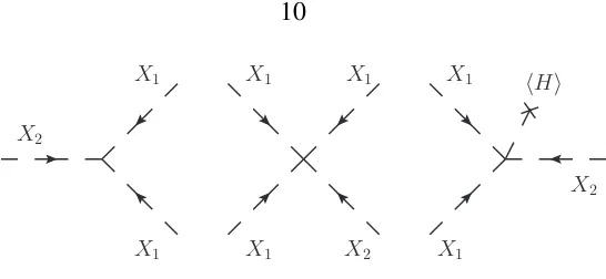
Baryon number violation will arise from terms in the scalar potential, so we need to take into account just the models whose scalar quantum numbers are compatible in the sense that they allow scalar interactions that violate baryon number. For scalars cou-pling to standard model fermion bilinears there are three types of scalar interactions which may violate baryon number: 3-scalarX1X1X2, 4-scalarX1X1X1X2, and 3-scalar with a HiggsX1X1X1H or X1X1X2H, where the Higgs gets a vacuum expectation value (vev) (Fig. 2.3).
hHi
X2
X1
X1
X1
X1
X1
X2
X1
X1
[image:16.612.174.447.70.196.2]X2
Figure 2.3: Scalar interactions which may generate baryon number violation.
X1
X1
X1
d e+
¯
ν
d ν¯
d
hHi
Figure 2.4: Interaction which leads to proton decay, p → π+π+e−νν, for X 1 = (¯3,2,−1/6).
X1X1X1H includes just one new scalar (¯3,2,−1/6), but it gives proton decay via p →
π+π+e−νν (Fig. 2.4). Note that a similar diagram withhHi replaced byX
2 allows us to ignore scalars with the same electroweak quantum numbers as the Higgs and coupling to
¯
QuandQd¯ ,X2 = (1,2,1/2)and(8,2,1/2), as these will produce tree level proton decay as well. The other two baryon number violating models with an interaction termX1X1X2H are: X∗
1 = (3,1,−1/3), X2 = (¯3,2,−7/6)and X1 = (3,1,−1/3), X2∗ = (¯3,2,−1/6). As argued earlier, such quantum numbers forX1also induce tree-level proton decay, so we disregard them.
[image:16.612.240.365.249.366.2]but only the first three models contribute to nn¯ oscillations at tree-level due to the sym-metry properties of the Yukawas. Note that a choice of normalization for the sextet given by,
(Xαβ) =
˜
X11 X˜12/√2 X˜13/√2 ˜
X12/√2 X˜22 X˜23/√2 ˜
X13/√2 X˜23/√2 X˜33
(2.1)
leads to canonically normalized kinetic terms for the elementsX˜αβ and the usual form of
the scalar propagator with symmetrized color indices. Unless otherwise stated, we will be using 2-component spinor notation. Parentheses indicate contraction of 2-component spinor indices to form a Lorentz singlet.
Model 1. X1 = (¯6,1,−1/3), X2 = (¯6,1,2/3)
L = −gab
1 X
αβ
1 Q
a Lα Q
b Lβ
−gab
2 X
αβ
2 (d
a Rαd
b Rβ)
−g0ab
1 X
αβ
1 (u
a Rαd
b
Rβ) +λX αα0
1 X
ββ0
1 X
γγ0
2 αβγα0β0γ0 (2.2)
Model 2. X1 = (¯6,3,−1/3), X2 = (¯6,1,2/3)
L = −gab
1 X
αβA
1 (QaLα τAQbLβ)−gab2 X
αβ
2 (daRαdbRβ)
+λXαα0A
1 X
ββ0A
1 X
γγ0
2 αβγα0β0γ0 (2.3)
Here the matrix τA is symmetric. Because the first and second terms have symmetric
color structures, g1 and g2 must be symmetric in flavor. The weak triplet X1 has com-ponents which introduce bothK0-K¯0 andD0-D¯0 mixing. As in model 1, the interaction involvingg2will introduceK0-K¯0 mixing viaX2 exchange.
Model 3. X1 = (¯6,1,2/3), X2 = (¯6,1,−4/3)
L = −gab
1 X
αβ
1 (d
a Rαd
b
Rβ)− g ab
2 X
αβ
2 (u
a Rαu
b Rβ)
+λXαα0
1 X
ββ0
1 X
γγ0
2 αβγα0β0γ0 (2.4)
Both terms have symmetric color structures and no weak structure, so g1 andg2 must be symmetric in flavor. In this model, the interactions involving g1 and g2 each have the po-tential to introduce neutral meson-antimeson mixing. For example, theg1 interaction will induceK0-K¯0mixing whileg
2 will induceD0-D¯0mixing.
Model 4. X1 = (3,1,2/3), X2 = (¯6,1,−4/3)
L = −gab
1 X1α daRβd b Rγ
αβγ
−gab
2 X
αβ
2 (u
a Rαu
b Rβ)
+λX1αX1βX2αβ (2.5)
symmet-ric and so we will get D0-D¯0 mixing as in model 3. Although this model does not have
nn¯ oscillations, there are still baryon number violating processes which would constrain this model – for example, the process pp → K+K+. This has been searched using the Super-Kamiokande detector looking for the nucleus decay16O→ 14CK+K+[7]. Had we includedνR, model 4 would have been excluded by tree-level scalar exchange.
Now, a similar line of reasoning applies to the case where we have a quartic scalar inter-action termX1X1X1X2. The only models violating baryon number which don’t generate proton decay (or bound neutron decay) are discussed briefly below. These last five models have dinucleon decay to leptons, but don’t contribute to tree-levelnn¯oscillations by virtue of their coupling to leptons.
Model 5. X1 = (¯6,1,−1/3), X2 = (1,1,1)
L = −gab
1 X
αβ
1 Q
a Lα Q
b Lβ
−gab
2 X2(LaLL b L)
−g0ab
1 X
αβ
1 (u
a Rαd
b Rβ)
+λXαα0
1 X
ββ0
1 X
γγ0
1 X2αβγα0β0γ0 (2.6)
Similar arguments to those for the previous models tell us thatg1 andg2 must be antisym-metric in flavor.
Model 6. X1 = (¯6,3,−1/3), X2 = (1,1,1)
L = −g1abX
αβA
1 (Q
a Lα τ
A
QbLβ)− g ab
2 X2(LaLL b L)
+λX1αα0AX
ββ0B
1 X
γγ0C
1 X2ABCαβγα0β0γ0 (2.7)
Model 7. X1 = (¯6,3,−1/3), X2 = (1,3,1)
L = −gab
1 X
αβA
1 (QaLα τAQbLβ)−g2abX2A(LaLτALbL)
+λXαα0A
1 X
ββ0B
1 X
γγ0C
1 X2Dαβγα0β0γ0
×(δABδCD+δACδBD+δADδBC) (2.8)
Once again, as in model 2, we have a symmetricg1. The couplingg2 must be symmetric in flavor as well.
Model 8. X1 = (¯6,1,2/3), X2 = (1,1,−2)
L = −gab
1 X
αβ
1 (d
a Rαd
b Rβ)−g
ab
2 X2(eaRe b R)
+λXαα0
1 X
ββ0
1 X
γγ0
1 X2αβγα0β0γ0 (2.9)
As in model 1,g1 must be symmetric. The couplingg2must also be symmetric in flavor.
Model 9. X1 = (3,1,2/3), X2 = (1,1,−2)
L = −gab
1 X1α(daRβd b Rγ)
αβγ
−gab
2 X2(eaRe b R)
+λX1αX1βX1γX2αβγ (2.10)
By comparison with model 4, we see thatg1must be antisymmetric in flavor. The coupling
2.3
Phenomenology of model 1
In this section we present a detailed analysis of model 1. The corresponding calculations for the other models can be performed in a similar manner. Our work is partly motivated by the recently proposednn¯ oscillation experiment with increased sensitivity [8]. In addition to
nn¯ oscillations, we also analyze the cosmological baryon asymmetry generation in model 1 as well as flavor and electric dipole moment constraints. A brief comment on LHC phenomenology is made.
2.3.1
Neutron-antineutron oscillations
The topic ofnn¯oscillations has been explored in the literature in various contexts. For some of the early works on the subject see [9, 10, 11, 12]. Recently, a preliminary study of the required hadronic matrix elements using lattice QCD has been carried out [13]. Reference [14] claims that a signal ofnn¯oscillations has been observed.
The scalar content of model 1 we are considering is similar to the content of a unified model explored in [15]. The transition matrix element,
∆m=hn¯|Heff|ni, (2.11)
leads to a transition probability for a neutron at rest to change into an antineutron after time
tequal toPn→n¯(t) = sin2(|∆m|t).
Neglecting the couplingg1in the Lagrangian (2.2) (for simplicity) the effective|∆B|= 2Hamiltonian that causesn¯noscillations is,
Heff = − (g011
1 )2g112 λ 4M4
1M22
dα˙
Rid
˙
β Ri0u
˙
γ Rjd
˙
δ Rj0u
˙
λ Rkd
˙
χ
Rk0α˙β˙γ˙δ˙λ˙χ˙ ×ijki0j0k0 +i0jkij0k0+ij0ki0jk0 +ijk0i0j0k
+ h.c.
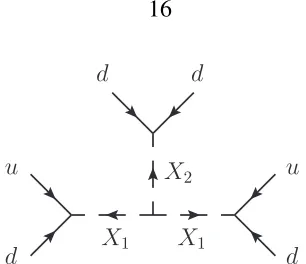
X2
X1 X1
d u
d u
[image:22.612.226.379.71.203.2]d d
Figure 2.5: Interaction which leads to neutron-antineutron oscillations.
where Latin indices are color and Greek indices are spinor. It arises from the tree-level diagram in Fig. 2.5 (see, for example [16]). We have rotated the couplingsg0
1 andg2 to the quark mass eigenstate basis and adopted a phase convention whereλ is real and positive. We estimate∆musing the vacuum insertion approximation [17]. This relates the required
nn¯ six quark matrix element to a matrix element from the neutron to the vacuum of a three quark operator. The later matrix element is relevant for proton decay and has been determined using lattice QCD methods. The general form of the required hadronic matrix elements is,
h0|dα˙
Rid
˙
β Rju
˙
γ
Rk|n(p, s)i=−
1 18β ijk
α˙γ˙uβ˙
R(p, s) +
˙
βγ˙uα˙
R(p, s)
. (2.13)
Here uR is the right-handed neutron two-component spinor and the Dirac equation was
used to remove the term proportional to the left-handed neutron spinor. The constantβwas determined using lattice methods in Ref. [18] to have the value β ' 0.01 GeV3
. In the vacuum insertion approximation to Eq. (2.11) we find (see Appendix 2.A),
|∆m|= 2λβ2|(g 011 1 )2g211| 3M4
1M22
. (2.14)
and yields a similar result. The current experimental limit on∆mis [20],
|∆m|<2×10⁻³³GeV. (2.15)
For scalars of equal mass,M1 =M2 ≡M, and the values of the couplingsg1011=g211= 1,
λ=M, one obtains,
M &500 TeV. (2.16)
If, instead, the masses form a hierarchy, the effect onnn¯ oscillations is maximized if we chooseM2 > M1. AssumingM1 = 5 TeV (above the current LHC reach) andλ = M2 this yields,
M2 &5×10¹³GeV. (2.17)
Note thatλ=M2is a reasonable value for this coupling since integrating outM2then gives a quartic X1 interaction term with a coupling on the order of one. Of course, this model does have a hierarchy problem so having the Higgs scalar and theX1 light compared with
X2requires fine tuning.
Experiments in the future [8] may be able to probenn¯ oscillations with increased sen-sitivity of|∆m| '7×10⁻³⁵GeV. If no oscillations are observed, the new limit in the case of equal masses will be,
M &1000 TeV. (2.18)
On the other hand, havingM1 = 5 TeVwould push the mass of the heavier scalar up to the GUT scale, leading to the following constraint on the second scalar mass,
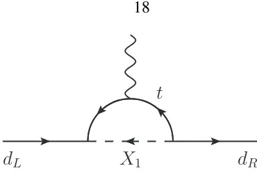
d
Rd
LX
1 [image:24.612.204.389.70.196.2]t
Figure 2.6: Diagram contributing to the electric dipole moment of the down quark.
We note, however, that in Section 2.3.2 we show that M1 on the order of a few TeV is disfavored by the electric dipole moment constraints.
2.3.2
LHC, flavor and electric dipole moment constraints
If the mass of the scalarX1 is small enough, it can be produced at the LHC through both single and pair production. Detailed analyses have been performed setting limits on the mass ofX1from such processes [21, 22, 23]. A recent simulation [21] shows that 100fb−1 of data from the LHC running at 14 TeV center of mass energy can be used to rule out or claim a discovery of X1 scalars with masses only up to approximately 1 TeV, even when the couplings to quarks are of order1. Our earlier choice ofM1 = 5 TeVused to estimate the constraint onM2 fromnn¯oscillations lies well within the allowed mass region.
Some of the most stringent flavor constraints on new scalars come from neutral meson mixing and electric dipole moments. The fact that in model 1,X1couples directly to both left- and right-handed quarks means that at one loop the top quark mass can induce the chirality flip necessary to give a light quark edm, putting strong constraints on this model even whenX1 is at the 100 TeVscale. The diagram contributing to the edm of the down quark is given in Fig. 2.6. We find (see Appendix 2.B),
|dd| '
mt
6π2M2 1
log
M2 1
m2
t
Im[g
31 1 (g
031 1 )
∗
]
e cm. (2.20)
contribution to the neutron edm because of the top quark mass factor. All Yukawa couplings in this section are in the mass eigenstate basis.
Using SU(6) wavefunctions, this can be related to the neutron edm via dn = 43dd−
1 3du '
4
3dd. The present experimental limit is [24],
dexp
n <2.9×10
−26 e cm.
(2.21)
AssumingM1 = 500 TeV, neutron edm measurements imply the bound
Im[g311 (g0311 )∗] .
6 × 10⁻³. Furthermore, for observable n¯n oscillation effects with M
2 being close to the GUT scale we need M1 ≈ 5 TeV. In such a scenario the edm constraint requires
Im[g131(g0
31 1 )
∗]
.10−6.
Another important constraint on the parameters of model 1 is provided byK0-K¯0 mix-ing. Integrating outX2generates an effective Hamiltonian,
Heff =
g22 2 (g211)
∗
M2 2
(sRαsRβ)(d∗Rαd
∗β R)
→ g
22 2 (g211)
∗
2M2 2
( ¯dαRγ µ
sRα)( ¯dβRγµsRβ), (2.22)
where in the second line we have gone from two- to four-component spinor notation (see Appendix 2.C). This gives the following constraints on the couplings [25],
Re
g222 g 11 2
∗
<1.8×10⁻⁶ M2 1 TeV 2 , (2.23) Im
g222 g 11 2
∗
<6.8×10⁻⁹
M2 1 TeV
2
. (2.24)
If we set M2 to 500 TeV, this corresponds to an upper bound on the real and imaginary parts ofg22
2 (g211) ∗
X2
X1
X1
X2 X2′
X1
X1
dR
dR
X2
dR
dR
X2 X2′
dR
dR X1
[image:26.612.153.458.71.303.2]X1
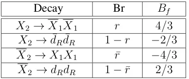
Figure 2.7: Diagrams corresponding to the decay ofX2. The diagrams on top contribute to the∆B = 2decays, while the diagrams on bottom contribute to∆B = 0.
Decay Br Bf
X2 →X1X1 r 4/3
X2 →d¯Rd¯R 1−r −2/3
X2 →X1X1 ¯r −4/3
X2 →dRdR 1−r¯ 2/3
Table 2.2: Branching ratios and final state baryon numbers for the decays of X2 and X2 which contribute to the baryon asymmetry in the coupling hierarchyλ,˜λg2,g˜2.
2.3.3
Baryon asymmetry
We now investigate baryon number generation in model 1. B andLviolating processes in cosmology have been studied in the literature in great detail (for early works, see [26, 27]). We treat X2 as much heavier than X1 and use two different X2’s to get a CP violating phase in the one-loop diagrams that generate the baryon asymmetry. For this calculation
[image:26.612.210.404.354.435.2]violating decays ofX2. Rotating theX fields to make the couplingsλ and˜λreal we find (see Appendix 2.D),
Γ(X2 →X1X1) = 3λ
8πM2
λ−λ˜ M
2 2 4π(M2
2 −M˜22)
Im(Tr(g†2˜g2))
,
Γ(X2 →X1X1) = 3λ
8πM2
λ+ ˜λ M
2 2 4π(M2
2 −M˜22)
Im(Tr(g2†g˜2))
. (2.25)
The net baryon number produced perX2X2pair is (see, Table 2.2),
∆nB = 2(r−r¯)
= 6
πTr(g†2g2) 1 ˜
M2 2 −M22
Imhλλ˜∗Tr(g†2˜g2)
i
, (2.26)
where we have used the fact thatCP T invariance guarantees the total width ofX2 andX¯2 are the same. Given our choice of hierarchy for the couplings, we have approximated the total width as coming from the tree-level decay ofX2to antiquarks. A similar result in the context ofSO(10)models was obtained in Ref. [15].
Even with just one generation of quarks, the CP violating phase cannot be removed from the couplingsλ, ˜λ, g2, ˜g2 and a baryon asymmetry can be generated at one loop. At first glance this is surprising since there are four fields, X2,X˜2, X1 anddRwhose phases
can be redefined and four relevant couplings. However, this can be understood by looking at the relevant Lagrangian terms,g2X2dd,˜g2X˜2dd,λX1X1X2and˜λX1X1X˜2. The problem reduces to finding solutions to the following matrix equation,
2 1 0 0 2 0 1 0 0 1 0 2 0 0 1 2
φX1 φX2 φX˜2
φd = φλ
φ˜λ
φg2 φ˜g2
, (2.27)
two equations to remove phases for the couplingg2,g˜2. We therefore obtainφλ˜2 −φλ2 = φX˜2 −φX2 andφ˜g2 −φg2 = φX˜2 −φX2. Those two equations cannot be simultaneously
fulfilled for arbitraryφλ,φ˜λ,φg2,φ˜g2.
The baryon number generated in the early universe can be calculated from Eq. (2.26) by following the usual steps (see, for example, [28]). Out of equilibrium decay ofX2 and
¯
X2is most plausible if they are very heavy (e.g.∼1012GeV). However, to get measurable
nn¯oscillation in this case,X1would have to be light – a case that is disfavored by neutron edm constraints, since it requires some very small dimensionless couplings.
2.4
Conclusions
We have investigated a set of minimal models which violate baryon number at tree-level without inducing proton decay. We have looked in detail at the phenomenological aspects of one of these models (model 1) which can havenn¯oscillations within the reach of future experiments. When all the mass parameters in model 1 have the same value, M, and the magnitudes of the Yukawa couplings g011
1 and g211 are unity, the present limit on n¯n oscillations implies that M is greater than 500 TeV. For M = 500 TeV, the neutron edm and flavor constraints give Im[g31
1 (g 031 1 )
∗] < 6
× 10−6, Re[g22 2 (g211)
∗] < 0.45, and
Im[g22
2 (g112 )∗] < 1.7×10⁻³ which indicates that some of the Yukawa couplings and/or their phases must be small if nn¯ oscillations are to be observed in the next generation of experiments. Of course even in the standard model some of the Yukawa couplings are small.
There are two other models (model 2 and model 3) that have nn¯ oscillations at tree-level. Similar conclusions can be drawn for them, although the details are different. In models 2 and 3, exchange of a single X1 does not give rise to a one-loop edm of the neutron. However,K0-K¯0 mixing can occur from tree-levelX
1 exchange.
Appendix
2.A
Vacuum insertion approximation
We are trying to evaluate
hn¯(p, s)|Heff|n(p, s)i (2.28)
where
Heff = − (g011
1 )2g112 λ 4M4
1M22
dα˙
Rid
˙
β Ri0u
˙
γ Rjd
˙
δ Rj0u
˙
λ Rkd
˙
χ
Rk0α˙β˙γ˙δ˙λ˙χ˙ ×ijki0j0k0 +i0jkij0k0+ij0ki0jk0 +ijk0i0j0k
+ h.c. (2.29)
using lattice results relevant to the matrix element
h0|dα˙
Rid ˙ β Rju ˙ γ
Rk|n(p, s)i=−
1 18β ijk
α˙γ˙uβ˙
R(p, s) +
˙
βγ˙uα˙
R(p, s)
. (2.30)
The coefficient in front of the right-hand side of this equation is chosen to make connection with the lattice result in Ref. [18] which includes the contraction withijk
˙
αγ˙.
To estimate the matrix element Eq. (2.28), we look for rearrangements of the operator Heff which upon inserting the vaccum states|0ih0|would give matrix elements of the form in Eq. (2.30). For example,Heff includes quark operators which can be rearranged as
dα˙
Rid
˙
β Ri0u
˙
γ Rjd
˙
δ Rj0u
˙
λ Rkd
˙
χ
Rk0 =−dαRi˙ d ˙
β Ri0u
˙
γ Rjd
˙
δ
Rj0dχRk˙ 0u ˙
λ
Note that there are 42 21 = 12of these rearrangements possible. Inserting|0ih0|into this choice gives a contribution
−hn¯|dα˙
Rid
˙
β Ri0u
˙
γ
Rj|0ih0|d
˙
δ
Rj0dχRk˙ 0u ˙
λ Rk|ni
=−
1 18
2 |β|2
ii0jj0k0k(α˙γ˙vβ˙ +β˙γ˙vα˙)(δ˙λ˙uχ˙ +χ˙λ˙uδ˙). (2.32)
Finally, we contract this structure with the remaining color and weak epsilon tensors in Eq. (2.29) using the identities
ijkijk = 6 (2.33)
imnjmn= 2δij (2.34)
ijkimn = 2δjmδkn−δjnδkm . (2.35)
It turns out this particular term contributes zero to the full matrix element because the color structure in Heff is symmetric under(i ↔ i0), (j ↔ j0), and(k ↔ k0). In fact, this reduces the number of non-zero contributions to just four of the twelve rearrangements. After evaluating these, we find the total contribution to be the result quoted in Eq. (2.14),
hn¯|Heff|i=|∆m|= 2λβ2| (g011
1 )2g211| 3M4
1M22
. (2.36)
2.B
Down quark edm
In computing the down-quark edm, we are looking for the coefficient of the operator
−L=idd
2 d¯Lσ
µν
FµνdR. (2.37)
Starting with the Lagrangian
L =−X1αβ
2gab1 (u
a Lαd
b Lβ) +g
0ab
1 (u
a Rαd
b Rβ)
we generate an effective Hamiltonian (integrating outX1)
Heff =−
gab
1 g10cd∗
M2
X1
(ua
LαdbLβ)(ucα
∗
R d dβ∗
R +u cβ∗
R d dα∗
R ) +h.c.
→ −g 13 1 g1031∗
M2
X1
(tLαdLβ)(tαR∗d β∗
R +t β∗
Rd α∗
R) +h.c. (2.39)
where in the second line we’ve focused on the top quark contribution which will dominate the dipole moment. Next, we write this using 4-component spinors by writing explicitly the spinor index contractions and then identifying the corresponding 4-component structure. That is,
(tLαdLβ) = tLαaabdLβb = (tTαCPLdβ) (2.40)
(tRαdRβ) = taLα˙ a˙b˙d
˙
b Lβ = (t
T
αCPRdβ). (2.41)
Taking the hermitian conjugate of the second line gives
dβ∗T(CP
R)†tα∗ = ¯dβγ0(CPR)†γ0¯tαT
= ¯dβγ0P†
RC
†
γ0¯tαT
= ¯dβγ0P†
Rγ
0γ0C†
γ0¯tαT
= ¯dβP LC¯tαT
= ¯dβCP
L¯tαT (2.42)
giving us an effective Hamiltonian in 4-component notation
Heff =−
gab
1 g10cd∗
M2
X1
(tT
αCPLdβ)( ¯dβCPL¯tαT + ¯dαCPLt¯βT). (2.43)
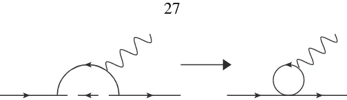
Figure 2.B.1: One-loop diagram contributing to the down quark edm.
diagram using just the first term inHeff is
h0|T{tα(x)a(CPL)abdβ(x)bbardβ(x)c(CPL)cd¯tα(x)d·¯tα(y)eγefµtα(y)f}|0i
= 3St
ae(x−y)S t
f d(y−x)γ µ
ef(CPL)ab(CPL)cddβ(x)bd¯β(x)c
= 3(CPL)TbaS t
ae(x−y)γ µ efS
t
f d(y−x)(CPL)Tdcdβ(x)bd¯β(x)c (2.44)
where we’ve left off the photon and defined
St
ab(x−y) = h0|T ta(x)¯tb(y)|0i. (2.45)
Note that the second term inHeff contributes in the same way, but without the color factor of 3.
Next, we evaluate
4 Z
˜
dq(CPL)T
i(/q+mt)
q2−m2
t
γµi(/q+/k+mt)
(q+k)2−m2
t
(CPL)T (2.46)
withq the incoming down quark momentum andk the outgoing photon momentum. The simplification of this is straightforward. Using
γµγν = 1 2{γ
µ, γν
}+ 1 2[γ
µ, γν] = 1 2{γ
µ, γν
we identify the piece coming fromσµν
−4mtPL
Z ˜
dq Cγ
µγνk νC
[q2−m2
t][(q+k)2−m2t]
→4imtPLCσµνkνC
Z ˜
dq 1
[q2−m2
t][(q+k)2−m2t]
= 4mtPLCσ
µνk νC
16π2 ln
M2 X1 m2 t . (2.48)
Finally, to correct for the photon we left off, we need to multiply by the top quark charge, 2
3 and a factor of 1
2 since this amplitude is generated by both terms inF
µν. This gives our
desired result,
idd
2 =i
mt
12π2M2
X1 ln M2 X1 m2 t Im(g13
1 g 031∗
1 ) (2.49)
2.C
K
0-
K
¯
0mixing
Here, we show explicitly the transformation between 2-component and 4-component nota-tion for the effective Hamiltonian inK0-K¯0mixing. We start by writing the spinor indices,
Heff =
g22 2 (g211)
∗
M2 2
(sRαsRβ)(d∗Rαd
∗β R)
=g 22 2 (g211)
∗
M2 2
(sa˙
Rαa˙b˙s
˙
b Rβ)(d
∗αa R abd
∗βb
R ). (2.50)
Next, we use the identity2a˙b˙ab =σ µ
aa˙σµbb˙to write this as
=g 22 2 (g211)
∗
2M2 2
(saRα˙ s
˙ b Rβd ∗αa R d ∗βb R )σ
µ aa˙σµbb˙
=g 22 2 (g211)
∗
2M2 2
(d∗Rαaσ µ aa˙s
˙
a Rα)(d
∗βb R σµbb˙s
˙
b Rβ)
=g 22 2 (g211)
∗
2M2 2
( ¯dα Rγ
µs
Rα)( ¯dβRγµsRβ) (2.51)
2.D
Absoptive part of
X
2decay
αβ αβ
µν
λσ µν
λσ
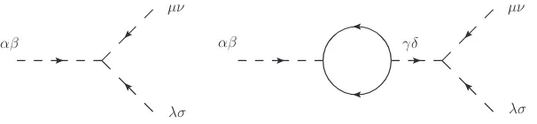
[image:35.612.151.454.139.209.2]γδ
Figure 2.D.1: Color structure of the relevant diagrams forX2 decay.
We start with the tree-level diagram in Fig. 2.D.1. The Feynman rule for this vertex gives
iMtree = 2iαµλβνσ . (2.52)
Because the same color structure appears in the 1-loop diagram, it will be useful to compute the decay amplitude for the tree-level process.
Γtree = 1 2
1 16πM2
1 6
X
initial colors
1 2
δα
α0δββ0+δβα0δαβ0
X
final colors
1 4 δ
µ
µ0δνν0 +δµν0δµν0
δλ
λ0δσσ0 +δλσ0δσλ0
×4|λ|2
αµλβνσα
0µ0λ0
β0ν0σ0
= 3
8πM2|
λ|2
(2.53)
The factors involving δ’s are used to symmetrize the amplitude over symmetric color in-dices, the factors of 12 is for identical final states, and the factors of 16 is for averaging over initial colors.
Next, we include the amplitude coming from the loop-diagram. The amplitude is
iMloop= 2λ0Tr[˜g †
2g2]αµλβνσ
1
M2 2 −M˜22
where theI(p2)is the loop factor
I(p2) = 2
Z
d4q (2π)4Tr
i/q q2+iPR
(−i)(/p+/q) (p+q)2+i
=−2
Z d4q
(2π)4 1
q2+i
1
(p+q)2+iTr
(−/q)PR(/p+/q)
=−2
Z d4q
(2π)4 1
q2+i
1
(p+q)2+i2q1·q2 (2.55) where we’ve definedq1 =−qandq2 =p+q. Now, the difference in decay rates between
X2 and X¯2 will depends only on the imaginary part of this loop integral which we can compute using the usual Cutkosky rules.
Disc
I(p2) =−2
Z
d4q 1 (2π)4
d4q 2 (2π)4(2π)
4δ(4)(q
1+q2−p)(−2πi)δ(q12)(−2πi)δ(q 2
2)2q1·q2 = 16π2
Z d4q 1 (2π)4δ(q
2 1)δ
(p−q1)2
M22 2 = 16π
2M2 2 2(2π)4
Z
d4q1
δ(q0
1 − |q~1|) 2q0
1
δ(M2
2 −q 0 1) 2M2 = 16π
2M2 2 2(2π)4
Z
d3q~ 1
δ(M2
2 − |q~1|)
M2
1 2M2 = 16π
2
4(2π)4
Z
4π|q~1|2d|q~1|δ(M22 − |q~1|)
= 16π 3
(2π)4
M2 2 2 = M 2 2
4π (2.56)
In the second line, we’ve integrated overq2 to eliminated theδ(4). In the third line, we’ve used an identity to rewrite the composition of a Dirac delta and another function.
Now, we use the fact that Disc [I(p2)] = 2iIm [I(p2)] to get the relevant part of our ampitude
iMloop=−2iλ0Tr[˜g †
2g2]αµλβνσ
1
M2 2 −M˜22
M2 2
Comparing this to our tree-level result tells us that
Γ = 3 8πM2
λ−iλ0Tr[˜g2†g2] 1
M2 2 −M˜22
M2 2 8π
2
' 3λ 8πM2
λ−λ0 M
2 2 4π(M2
2 −M˜22)
Im(Tr(g2†g˜2))
Chapter 3
Phenomenology of scalar leptoquarks
3.1
Introduction
Currently, the standard model describes most aspects of nature with remarkable precision. If there is new physics at the multi TeV scale (perhaps associated with the hierarchy puz-zle), it is reasonable to expect measurable deviations from the predictions of the standard model in the flavor sector. Amongst the experiments with very high reach in the mass scale associated with beyond the standard model physics are those that look for flavor violation in the charged lepton sector through measurements of the processes,µ→eγ[29] andµ→e
conversion [30, 31], and the search for electric dipole moments of the neutron, proton and electron.
Models with scalar leptoquarks can modify the rates for these processes. Simple models of this type have been studied previously in the literature, including their classification and phenomenology [32, 33, 34, 35, 36, 37, 38, 39].
violation in perturbation theory via leptoquark exchange. Of course there is baryon number violation through non-perturbative quantum effects since it is an anomalous symmetry. But this is a very small effect at zero temperature. Only two models fulfill this requirement. One of those two models gives a top mass enhanced µ → eγ decay rate. We perform an analysis of the phenomenology of this specific model, including the µ → eγ decay rate,
µ→ econversion rate, as well as electric dipole moment constraints focussing mostly on the regions of parameter space where the impact of the top quark mass enhancement is most important. For lepton flavor violating processes at higher energies such asτ → µγ, deep inelastic scattering e +p → µ(τ) +X, etc., the impact on the phenomenology of the top quark mass enhancement of charged lepton chirality flip is less dramatic and that is why we focus in this paper on low energy processes involving the lightest charged leptons. We also consider the effects of dimension five operators that can cause baryon number violation. We find that the two models without renormalizable baryon number violation can have such operators and, even if the operators are suppressed by the Planck scale, they may (depending on the values of coupling constants and masses) give rise to an unaccept-able level of baryon number violation. We discuss a way to forbid these dimension five operators.
3.2
Models
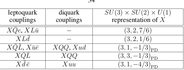
A general classification of renormalizable leptoquark models can be found in [32, 33]. However, in the spirit of our approach, in which we are interested in models with no proton decay from leptoquark exchange, a more useful list of possible interaction terms between the scalar leptoquarks and fermion bilinears is presented in [40], where those models that have tree-level proton decay are highlighted. The relevant models are listed in Table 3.1 below.
leptoquark diquark SU(3)×SU(2)×U(1) couplings couplings representation ofX
XQe¯ ,XLu¯ − (3,2,7/6)
XLd¯ − (3,2,1/6)
XQ¯L¯,Xu¯e¯ XQQ,Xud (3,1,−1/3)PD
XQ¯L¯ XQQ (3,3,−1/3)PD
[image:40.612.145.469.75.198.2]Xd¯e¯ Xuu (3,1,−4/3)PD
Table 3.1: Possible interaction terms between the scalar leptoquarks and fermion bilinears along with the corresponding quantum numbers. Representations labeled with the subscript “PD” allow for proton decay via tree-level scalar exchange.
Model I: X = (3,2,7/6).
The Lagrangian for the scalar leptoquark couplings to the fermion bilinears in this model is,
L = −λij uu¯
i RX
TLj L−λ
ij ee¯
i RX
†
QjL+ h.c. , (3.1)
where, X = Vα Yα , = 0 1 −1 0
, LL =
νL
eL
. (3.2)
After expanding theSU(2)indices it takes the form,
L = −λijuu¯ i
αR(VαejL−YανLj)−λijee¯ i R(V
†
αu j αL+Y
†
αd j
αL) + h.c. . (3.3)
Note that in this model the left-handed charged lepton fields couple to right-handed top quarks, and the right-handed charged lepton fields couple to left-handed top quarks. So a charged lepton chirality flip can be caused by the top mass at one loop.
The corresponding Lagrangian is,
L = −λijdd¯i RX
TLj
L+ h.c. , (3.4)
where we have used the same notation as in the previous case. Expanding the SU(2) indices yields,
L = −λijdd¯iαR(Vαe j
L−Yαν j
L) + h.c. . (3.5)
In model II the leptoquark cannot couple to the top quark, so there is nomtenhancement
in theµ → eγ decay rate. There is also nomb enhancement, and the one-loop effective
Hamiltonian forµ→eγ (after integrating out the massive scalars and the heavy quarks) is proportional to the muon mass. In addition, as mentioned in [40], this model does generate tree-level proton decay from its interaction with the Higgs field. For this reason, in the remainder of the paper we will focus entirely on model I.
3.3
Phenomenology
In this section we analyze some of the phenomenology of model I, i.e., X = (3,2,7/6). We concentrate only on those constraints which are most restrictive for the model and po-tentially most sensitive to the unusual top mass enhancement of the charged lepton chirality change, i.e., the ones coming from the following processes – muon decay to an electron and a photon, muon to electron conversion, and electric dipole moment of the electron.
3.3.1
Naturalness
matrix induced at one loop is given by,
∆mij 'λ˜3uiλ˜je3
3mt
16π2 log
Λ2
m2
V
, (3.6)
whereΛis the cut-off scale. To avoid unnatural cancellations between this loop contribu-tion to the lepton mass matrix and the tree-level lepton mass matrix we require,
|∆mij|.√mimj . (3.7)
For example, for a scalar of massmV = 50 TeVand a cut-off set at the GUT scale Eq. (3.6)
gives,
∆mij 'λ˜3uiλ˜ j3
e ×170 GeV,= (3.8)
which, combined with Eq. (3.7), yields the following constraint on the couplings,
|˜λ13
e λ˜
32
u |,|λ˜
23
e ˜λ
31
u |.4.3×10
−5 .
(3.9)
In the subsequent analysis we will include the constraint imposed by Eq. (3.7) by indicating which region of the plots is not favored by the naturalness considerations.
3.3.2
µ
→
eγ
decay
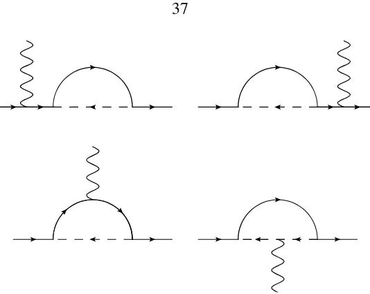
The relevant Feynman diagrams for this process are presented in Fig. 3.1. The uniqueness of model I is that, apart from the fact there is no tree-level proton decay, theµ → eγ rate is enhanced by the top quark mass. To our knowledge, such an enhancement of µ → eγ
was observed previously only in [36] in the context of anSU(2) singlet scalar leptoquark model. However, that model suffers from perturbative proton decay and the impact of the
mtenhancement was not focussed on.
Figure 3.1: Feynman diagrams contributing to the processµ→eγ.
diagrams in Fig. 3.1 (neglecting the terms proportional tome) is given by (see Appendix
3.A),
iM = − 3e mt 16π2m2
V
f(m2
t/m
2
V)kνµ(k)
× hλ˜13
e ˜λ
32
u ¯eR(p−k)σµνµL(p) + (˜λ31u )
∗
(˜λ23
e )
∗
¯
eL(p−k)σµνµR(p)
i
,(3.10)
where k is the photon four-momentum and is the photon polarization. The function
f(m2
t/m2V)is given by,
f(x) = 1−x
2+ 2xlogx 2(1−x)3 +
2 3
1−x+ logx
(1−x)2
, (3.11)
and the tilde over the couplings denotes that they are related by transformations that take the quarks and leptons to their mass eigenstate basis through the following 3×3matrix transformations,
˜
λu =U(u, R)†λuU(e, L), λ˜e=U(e, R)†λeU(u, L), (3.12)
eigenstate up-type quarks by the matrix U(u, R), the left-handed up quarks in the La-grangian are related to the left-handed mass eigenstate up-type quarks by the matrixU(u, L), etc.
Theµ→eγ decay rate is,
Γ(µ→eγ) = 9e 2λ2m2
tm3µ
2048π5m4
V
f(m2
t/m 2 V) 2 , (3.13) where, λ≡ r 1 2 λ˜13e λ˜32u
2 +1 2 ˜λ31u λ˜23e
2
. (3.14)
Fig. 3.2 shows the relation between λ and the scalar leptoquark mass. This dependence was plotted for the µ → eγ branching ratio equal to the current upper limit of Br(µ → eγ)'2.4×10⁻¹²reported by the MEG experiment, and the prospective MEG sensitivity of Br(µ → eγ) ' 5.0×10⁻¹³. It shows that the experiment will be sensitive to scalar leptoquark masses at the hundred TeV scale for small values of the couplings.
For very small x, f(x) → f˜(x) = 2
3logx. This is a reasonable approximation in the range ofxwe are interested in. For example,f˜(10−8)/f(10−8)'1.1.
3.3.3
µ
→
e
conversion
The effective Hamiltonian for theµ→econversion arises from two sources,
Heff =H (a) eff +H
(b)
eff . (3.15)
The first is the dipole transition operator that comes from the loop diagrams which are responsible for theµ→eγ decay, given by,
Heff(a) =
3e mt
32π2m2
V
f(m2t/m
2
V)
× hλ˜13
e ˜λ
32
u e¯RσµνµLFµν+ (˜λ31u )
∗
(˜λ23
e )
∗
¯
eLσµνµRFµν
i
0 10 20 30 40 50 60 70 80 0
10-5 2´10-5 3´10-5 4´10-5 5´10-5
mV@TeVD
Λ BrHΜ®eΓL=2.4´10
-12
BrHΜ®eΓL=5.0´10-13 NOT FAVORED BY NATURALNESS
Figure 3.2: The combination of couplings λ from Eq. (3.14) as a function of the scalar leptoquark mass for two values of theµ→eγbranching ratio relevant for the MEG exper-iment. The shaded region consists of points which do not satisfy Eq. (3.7).
Using the following Fierz identities (for spinors),
(¯u1Lu2R)(¯u3Ru4L) =
1 2(¯u1Lγ
µ
u4L)(¯u3Rγµu2R),
(¯u1Lu2R)(¯u3Lu4R) =
1
2(¯u1Lu4R)(¯u3Lu2R) (3.17) + 1
8(¯u1Lσ
µνu
4R)(¯u3Rσµνu2L),
we arrive, after integrating out the heavy scalar leptoquarks (at tree level), at the second part of the effective Hamiltonian,
Heff(b) = 1 2m2
V
˜
λ12
u (˜λ11u )
∗
(¯eLγµµL)(¯uαRγµuαR)
+˜λ11e λ˜
12
u
h
CS(µ)(¯eRµL)(¯uαRuαL) +
1
4CT(µ)(¯eRσ
µν
µL)(¯uαRσµνuαL)
i
+ ˜λ11e (˜λ
21
e )
∗
(¯eRγµµR)(¯uαLγµuαL)
+(˜λ21e )
∗
(˜λ11u )
∗h
CS(µ)(¯eLµR)(¯uαLuαR)+
1
4CT(µ)(¯eLσ
µν
µR)(¯uαLσµνuαR)
i
+ 1 2m2
Y
(˜λeVCKM)11
(˜λeVCKM)21
∗
0 50 100 150 200 250 300 0
10-5 2´10-5 3´10-5 4´10-5 5´10-5
mV@TeVD
Λ
BrHΜ®e in AlL=10-17 NOT FAVORED BY NATURALNESS
BrHΜ®e in AlL=10-16
BrHΜ®eΓL=10-14
Figure 3.3: The combination of couplings λ from Eq. (3.14) as a function of the scalar leptoquark mass for two values of theBr(µ → econversion in Al)relevant for the Mu2e experiment. The thin solid line, corresponding to Br(µ → eγ) = 10−14, is included for reference. The shaded region consists of points which do not satisfy Eq. (3.7).
The CKM matrix arises whenever a coupling to the left-handed down-type quark appears. In Eq. (3.18) the contribution of the heavy quarks, as well as the contribution of the strange quark, are in the ellipses. Since the operators qq¯ and qσ¯ µνq do require renormalization,
their matrix elements develop subtraction point dependence that is cancelled in the leading logarithmic approximation by that of the coefficients CS,T. Including strong interaction
leading logarithms we get,
CS(µ) =
αs(mV)
αs(µ)
−12/(33−2Nq)
(3.19)
and
CT(µ) =
αs(mV)
αs(µ)
4/(33−2Nq)
, (3.20)
whereNq = 6is the number of quarks with mass belowmV. In order to match the effective
Hamiltonian (3.18) to the Hamiltonian at the nucleon level and use this to compute the conversion rate, we follow the steps outlined in [41, 42].
The current experimental limit isBr(µ→ econversion in Au) <7.0×10⁻¹³[43]. How-ever, here we focus on the prospective Mu2e experiment [30], which has a sensitivity goal of5×10−17. The COMET experiment [31] aims for comparable sensitivity in later stages. We use the total capture rate for 27
13Alof ωcapture = 0.7054×10⁶ s−1 [44] to switch from theµ→econversion rate to a branching ratio.
Apart from coupling constant factors, the contribution to theµ→ econversion ampli-tude from Heff(a) is enhanced over the contribution to the amplitude from H(b)eff roughly by (mt/mµ)(3e2/32π2) log(m2V/m2t)∼10, formV in the hundred TeV range.
Our results show that in some regions of parameter space the Mu2e experiment will be able to constrain leptoquark couplings with similar precision to what can be done with an experiment which is sensitive to a branching ratio forµ → eγ of around 10−14. In other regions the Mu2e experiment is likely to give a more powerful constraint for such aµ→eγ
branching ratio, for example, when the Yukawa couplings are strongly hierarchical and the top quark loop is very suppressed.
To show graphically the contributions to the branching ratio originating from terms in the effective Hamiltonian with different structures, we set all the couplings to zero apart fromλ˜13
e ,λ˜23e ,˜λ31u ,λ˜32u ,˜λ11u ,λ˜12u for simplicity, i.e., we leave only the couplings relevant for
theµ→eγ decay and one of the vector contributions toH(b)eff.
Note that the heavy quark contributions are suppressed byΛQCD/mQ, low energy
phe-nomenology suggests that the strange quark contribution is small, and furthermore the ten-sor contributions are not enhanced by the atomic number of the target.
In addition, we consider only real couplings and define κ ≡ ˜λ11
u λ˜12u . We also assume
˜
λ13
e ˜λ32u = ˜λ31u λ˜23e =λ, so that we can plotλas a function of the scalar leptoquark massmV
for a given value of the ratio,
r≡ κ
λ =
˜
λ11
u λ˜12u
q
1
2(˜λ13e λ˜32u )2+
1
2(˜λ31u λ˜23e )2
. (3.21)
0 100 200 300 400 500 0
10-5 2´10-5 3´10-5 4´10-5 5´10-5
mV@TeVD
Λ r=10 r=1
NOT FAVORED BY NATURALNESS
r=100 r=200
BrHΜ®e conv.in AlL=10-16
Figure 3.4: The combination of couplings λ from Eq. (3.14) as a function of the scalar leptoquark mass for a branching ratio Br(µ → e conversion in Al) = 10−16 and four different positive values of the ratio of the couplingsrfrom Eq. (3.21). The shaded region consists of points which do not satisfy Eq. (3.7).
0 100 200 300 400 500
0 10-5 2´10-5 3´10-5 4´10-5 5´10-5
mV@TeVD
Λ r=-1 r=-10
NOT FAVORED BY NATURALNESS
r=-100 r=-200
BrHΜ®e conv.in AlL=10-16
Figure 3.5: Same as Fig. 3.4, but for negative values ofr.
and two values of the branching ratioBr(µ→econversion in Al) = 10−16,10−17.
0 200 400 600 800 1000 0
10-5 2´10-5 3´10-5 4´10-5 5´10-5
mV@TeVD
Λ r=10 r=1
NOT FAVORED BY NATURALNESS
r=100 r=200
BrHΜ®e conv.in AlL=10-17
Figure 3.6: Same as Fig. 3.4, but for a branching ratio Br(µ → e conversion in Al) = 10−17.
If the interference is constructive, the curve moves down with increasingrsince a smaller value of the couplingλ is required to achieve a given branching ratio (Figs. 3.5 and 3.7). In the case of a destructive interference, the curves move up until a value of r is reached for which the two contributions are the same (Figs. 3.4 and 3.6). As estimated before, this occurs forr ≈ 10. Increasing r further brings the curves back down, since theH(b)eff contribution becomes dominant.
Large values of r are expected if the Yukawa couplings of X exhibit a hierarchical pattern like what is observed in the quark sector; κchanges generations by one unit while the product of couplings in λ involves changing generations by three units. Finally, we note that for all the curves in the plots above the Yukawa couplings are well within the perturbative regime.
3.3.4
Electron EDM
0 200 400 600 800 1000 0
10-5 2´10-5 3´10-5 4´10-5 5´10-5
mV@TeVD
Λ r=-1 r=-10
NOT FAVORED BY NATURALNESS
r=-100 r=-200
BrHΜ®e conv.in AlL=10-17
Figure 3.7: Same as Fig. 3.5, but for a branching ratio Br(µ → e conversion in Al) = 10−17.
chirality flip necessary to give an electron EDM. We find that,
|de| '
3e mt
16π2m2
V
f(m2
t/m
2
V)
Im[˜λ13e ˜λ31u ]
. (3.22)
The present electron EDM experimental limit [45] is,
|de|<10.5×10⁻²⁸ecm. (3.23)
We can write the dipole moment in terms of the branching ratio,Br(µ → eγ), giving the constraint
Im[˜λ13e λ˜31u ]
λ
p
Br(µ→eγ)<2.0×10⁻⁷ .
(3.24)
For example, if model I gave a branching ratio equal to the current experimental bound of Br(µ → eγ) < 2.4×10⁻¹², this would correspond to the constraint on the couplings of
Im[˜λ13e ˜λ31u ]
/λ < 0.13. Fig. 3.8 shows the relation between the parameters
Im[˜λ13e λ˜31u ]
0 100 200 300 400 0
10-6 2´10-6 3´10-6 4´10-6
mV@TeVD
È
Im
H
Λe
13
Λu
31 LÈ
NOT FAVORED BY NATURALNESS
ÈdeÈ=10-27e cm
ÈdeÈ=10-28e cm
[image:51.612.152.465.71.286.2]ÈdeÈ=10-29e cm
Figure 3.8: The combination of couplings Im[˜λ13e λ˜31u ]
as a function of the scalar lepto-quark mass for three different values of the electron EDM. The shaded region consists of points which do not satisfy Eq. (3.7).
3.4
Baryon number violation and dimension five
opera-tors
Tree-level renormalizable interactions are not the only possible source of baryon number violation. It might also occur through higher-dimensional nonrenormalizable operators. In the standard model, proton decay is restricted to operators of mass dimension six or higher. However, the scalar leptoquark models we consider exhibit proton decay through dimension five operators.
Let’s first consider model I, in whichX = (3,2,7/6). Although it doesn’t give proton decay at tree level, one can construct the following dimension five operator,
OI =
1 Λg
ab
daRαd b Rβ(H
†
Xγ)αβγ . (3.25)
s
d
hHi
X
Q, u
[image:52.612.196.407.69.206.2]e, L
Figure 3.9: Feynman diagram representing proton decay in model I.
constants to unity, we estimate the baryon number violating nucleon decay rate caused by this operator to be,
Γp ≈2×10−57
50 TeV
mV
4
MPL Λ
2
GeV. (3.26)
Since the current experimental limit is Γexp
p < 2.7×10
−66 GeV[46], even if the scale of new physicsΛis equal to the Planck massMPLwhen the coupling constants are unity, this operator causes too large a proton decay rate formV .10 000 TeV.
In the case of model II, where X = (3,2,1/6), there are two dimension five baryon number violating operators,
OII(1) =
1 Λg
abua
RαdbRβ(H
†
Xγ)αβγ ,
OII(2) =
1 Λg
abua
RαebR(XβXγ)αβγ . (3.27)
The operatorOII(1) permits a nucleon decay pattern similar to the previous case, e.g.,n → e−π+andp→π+ν. Proton decay through the operatorO(2)
II is much more suppressed.
operatorsOI,O
(1)
II , andO
(2)
II are invariant under this transformation. However, we find that
imposing aZ3 discrete symmetry, with elements that are powers of exp[2πi(B −L)/3], forbids these dimension five operators and, thus, prevents the proton from decaying in this class of models. Note that gaugingB−Land spontaneously breaking the symmetry with a charge three scalar (at some high scale) leaves this unbroken discreteZ3gauge symmetry. It is not possible to use any discrete subgroup of B −L to forbid proton decays in the models from Table 3.1 which exhibit proton decay at tree level since all the interactions conserveB−L.
Finally, we would like to comment on the relation between this work and that of [40], where renormalizable models that have additional scalars and have baryon number viola-tion at tree level but not proton decay were enumerated and discussed. In these models none of the scalars were leptoquarks (they could rather be called diquarks or dileptons). However, if we permit higher dimension operators, then models 4 and 9 containing the scalarX = (3,1,2/3)(which has renormalizable diquark couplings), have dimension five leptoquark-type couplings,
OIII =
1 Λg
ab( ¯Qαa L H)e
b
RXα . (3.28)
This operator, combined with the renormalizable couplings ofX to two quarks, gives pro-ton decay with the rate estimated in Eq. (3.26). This observation restricts the parameter space of models 4 and 9 presented in [40] to the one in which either the color triplet scalar
Xis very heavy or its Yukawa couplings are small.