Robust dynamic cooperative games.

White Rose Research Online URL for this paper:

http://eprints.whiterose.ac.uk/89746/

Version: Accepted Version

Article:

Bauso, D. and Timmer, J. (2009) Robust dynamic cooperative games. International

Journal of Game Theory, 38. 23 - 36. ISSN 0020-7276

https://doi.org/10.1007/s00182-008-0138-1

[email protected] https://eprints.whiterose.ac.uk/ Reuse

Unless indicated otherwise, fulltext items are protected by copyright with all rights reserved. The copyright exception in section 29 of the Copyright, Designs and Patents Act 1988 allows the making of a single copy solely for the purpose of non-commercial research or private study within the limits of fair dealing. The publisher or other rights-holder may allow further reproduction and re-use of this version - refer to the White Rose Research Online record for this item. Where records identify the publisher as the copyright holder, users can verify any specific terms of use on the publisher’s website.

Takedown

If you consider content in White Rose Research Online to be in breach of UK law, please notify us by

(will be inserted by the editor)

Robust Dynamic Cooperative Games

D. Bauso1_{, J. Timmer}2

1

Dipartimento di Ingegneria Informatica, Universit`a di Palermo, V.le delle Scienze,

90128 Palermo, ITALY, e-mail:[email protected]

2

Department of Applied Mathematics, University of Twente, P.O. Box 217, 7500

AE Enschede, The Netherlands, e-mail:[email protected]

The date of receipt and acceptance will be inserted by the editor

Abstract Classical cooperative game theory is no longer a suitable tool

for those situations where the values of coalitions are not known with

cer-tainty. We consider a dynamic context where at each point in time the

coalitional values areunknown but bounded by a polyhedron. However, the

average value of each coalition in the long run is known with certainty. We

design “robust” allocation rules for this context, which are allocation rules

that keep the coalition excess bounded while guaranteeing each player a

cer-tain average allocation (over time). We also present a joint replenishment

application to motivate our model.

Keywordscooperative games, dynamic games, joint replenishment.

1 Introduction

Classical cooperative game theory is no longer a suitable tool for those

situ-ations where the values of coalitions are not known with certainty (see, e.g.,

Suijs and Borm (1999) [19], Suijset al.(1999) [20], Timmeret al.(2003) [22],

Timmer et al. (2005) [23]. In this paper we consider a sequence of games,

where, differently from Filar and Petrosjan (2000) [8] and Haurie (1975) [10],

theaverage coalitions’ values (over time) are known with certainty but the

instantaneous values areunknown but boundedby a polyhedron. This model

may be seen as a dynamic extension of the recently introduced cooperative

interval games (cf. Alparslan G¨oket al.(2008) [1–3]) where a coalition value

is a closed interval on the real line.

At each point in time a certain revenue is allocated to each player. In

general, these revenues will not meet the actual instantaneous value of the

coalitions. To keep track of this, an excess vector stores the difference

be-tween the instantaneous value of each coalition and the sum of the allocated

revenues to all its players. (This excess is different from the coalitional excess

that appears, e.g., in the definition of the nucleolus [15]).) We may

inter-pret this excess vector as the state variable describing the history of our

dynamic system. Under the assumption that the only information available

at each time is the excess of the coalitions, our goal is to design “robust”

allocation rules, i.e., allocation rules that i) keep the excess vector bounded

within a pre-defined thresholdǫat each time (we will refer to such rules as

time. Justification for keeping the excess vector bounded follows from the

observation that a fair allocation should not allocate maximum excess to the

same coalition each time. Our problem of interest may arise in a number

of real life situations as, for instance, in joint replenishment applications

(cf. Section 2.3). One may notice that our problem is similar in spirit to

classical problems in machine learning (cf. Cesa-Bianchi et al. (2006) [6],

Cesco (1998) [7] and Lehrer (2002) [12]). Therefore, after introducing our

allocation rule (or algorithm, since it is an iterative procedure), we compare

it to the algorithms proposed in [7,12].

This paper is organized as follows. In Section 2 we describe the problem.

In Section 3 we design the allocation rule. In Section 4 we compare our

algo-rithm to some existing algoalgo-rithms. In Section 5 we consider allocation rules

based on the Shapley value. Finally, in Section 6 we draw some conclusions.

2 Problem statement

2.1 Family of balanced games

We start by introducing the definition of a family of games with coalitions’

values lying on pre-assigned closed intervals. Let a game in coalitional form

< N, v > be given where N = {1, . . . , n} is a set of n players and v is

the characteristic function returning the value of each coalition S ⊆ N.

Henceforth let the inclusion S ⊆N mean “all coalitions of N except the

the empty set∅ and, with a little abuse of notation, let alsov∈Rmbe the

vector of coalitions’ values, namely,v= [v(S)]S⊆N.

Definition 1Afamily of games< N,V>is the set of games< N, v >

ob-tained whenv varies within a polyhedronV ={v∈Rm:vmin≤v≤vmax},

where the boundsvmin andvmax are given.

For the sake of simplicity, throughout this paper we always assumev≥0.

Also, for the sake of notation, we henceforth denote by 2N _{the family of}

subsets ofN. Let us recall the definition of a balanced map and a balanced

game for games < N, v > (see, e.g., Tijs (2003) [21, Def. 11.5]). A map

λ: 2N _{\ {∅} →R}+ _{is called a balanced map if}P

S⊆Nλ(S)eS =eN. Here,

R+is the set of nonnegative real numbers andeS _∈Rn_{is thecharacteristic}

vector for coalitionS witheS

i = 1 ifi∈S andeSi = 0 ifi∈N\S. Also, an

n-person game< N, v >is called abalanced game if for each balanced map

λ: 2N_{\ {∅} →R}+_,

X

S⊆N

λ(S)v(S)≤v(N). (1)

If the above condition is satisfied for each game v ∈ V, we say that the

polyhedron V describes a family of balanced games, as established more

formally in the next definition.

Definition 2A family of balanced games < N,Vb > is the set of games

< N, v >obtained when v varies within a polyhedron

Vb={v∈ V : condition (1) holds},

Sets of balanced games can also be found in the work of Kranichet al.

(2005) [11] and Lehrer (2002) [12].

Next, let us revisit the notions of core and allocation rules. Indicate with

∆n _{the simplex inR}n _{and recall that a game is balanced if and only if the}

core is nonempty [5,18]. By definition each game < N, v >with v ∈ Vb is

balanced, and so the coreC(v),

C(v) ={a∈Rn: a v(N) ∈∆

n_,X

i∈S

ai≥v(S) for allS⊆N},

is nonempty. This means that there exists an allocationa ∈C(v) ofv(n)

with the interpretation that no coalition has an incentive to split off from

the coalition N. Now, the problem is to find an allocation rule a(v) such

that a(v)∈C(v) for all games v∈ Vb. To solve this, first observe that the

core is a convex set described by linear equations and inequalities. For our

purpose it is useful to change all inequalities into equations. Therefore, we

first introduce a vector of nonnegative surplus variabless= [s1, . . . , sm−1]′

whereζ′ _{denotes the transposed of a given vectorζ. Each surplus variable}

corresponds to a coalition of players and describes the difference between

the allocated value and the coalitional value, P_i∈Sai−v(S). Notice that

we only needm−1 surplus variables becauseP_i∈Nai =v(N) due to the

efficiency condition of the core. Further, we introduce an incidence matrix

matrixA∈Rm×(n+m−1)defined by A=         B ¯ ¯ ¯ ¯ ¯ ¯ ¯ ¯ ¯ ¯ ¯ ¯ −I − − −−

0. . .0

        , (2)

where I is the (m−1)-dimensional identity matrix. Now, finding an

allo-cation rule ain the coreC(v) corresponds to finding a so-calledallocation

vector u∈Rn+m−1 _{in the set}

U(v) ={u:Au=v, u≥0} (3)

because if u ∈ U(v) then u = £_sa¤ for some a ∈ C(v). Observe that, in

general,U(v) is a polyhedron of dimensionn−1.

2.2 Dynamic system

Given the definition of family of balanced games, we now consider a sequence

of games that fluctuates in the bounded polyhedronVb. We denote this by

v(t), t= 1,2, . . .withv(t)∈ Vb for allt (4)

and v(t) = [v(t, S)]S⊆N is the vector of coalitional values. The values of

v(t) andv(t+ 1) are not correlated, which means that we cannot describe

transitions fromv(t) tov(t+1). This also implies that we cannot takev(t) as

a state variable and define dynamics (neither deterministic nor stochastic)

on it. On the contrary, it is realistic to assume that we know with certainty

theaverage vector of coalitions’ values v¯, being defined by

¯

v= lim

T−→∞ 1 T T X k=0

Obviously, ¯vcharacterizes the sequence of games under consideration.

Further, assume that allocations to players are made at a higher rate

than the rate of change of the coalitional values, which equals 1. Allowing

different rates means that he who allocates the revenues provides a faster

response in reply to the excesses of the coalitions. We will show later on that

faster allocations allow for lower excesses. More precisely, let the integer

number 1/Θ be the rate of allocations. Then Θ is the time between two

successive allocations. To facilitate our analysis, we stretch the time scale

by the rate 1/Θand consider a new sequence of games, namely

v(k) =v(t)Θ, k=t−1

Θ + 1, . . . , t

Θ, t= 1,2, . . . . (6)

This new sequence of games has the following interpretation. In the original

time interval (t−1, t] the vector of coalitional values equals v(t). We

dis-tribute these values equally over the 1/Θallocations that occur in this time

period, so this results in valuesv(t)Θ for each point in time where

alloca-tions are made. This way we can ensure that the total amount allocated to

the players in the new interval ((t−1)/Θ, t/Θ] does not exceed the available

amountv(t, N).

If we use the notation VΘ

b = Θ· Vb, the sequence of games (4)-(5), is

equivalent to the sequence of games

v(k), k= 1,2, . . .withv(k)∈ VΘ

b for eachk= 1,2, . . .

¯

v= limT−→∞_T1PTk=0v(k)

(7)

where ¯v=Θv¯. In the remainder of this paper, we will refer to the sequence

Now, denote by x(k+ 1) ∈ Rm a vector of variables describing the

aggregate coalition excesses over all previous gamesv(1), . . . , v(k) (the value

x(0) is the excess at time 0), i.e.,

x(k+ 1, S) =x(k, S) +X

i∈S

ai(k)−(sS(k) +v(k, S)) for all S⊆N , (8)

whereai(k) is the revenue allocated to playeriandsS(k) is a desired surplus

for coalition S. Roughly speaking, the coalition excess at time k is the

difference between the sum of the allocated revenues to the players of the

coalition and the value of the coalition increased by a desired surplus for that

coalition. The aggregate coalition excess x(k+ 1, S) is the coalition excess

summed over all previous gamesv(1), . . . , v(k) and therefore represents the

state of the system (x(k) describes the history of the system). We rewrite

equation (8) in the following matrix form

x(k+ 1) =x(k) +Au(k)−v(k), v(k)∈ VbΘ, k= 1,2, . . . , (9)

where u(k) = £a_s((k_k)₎¤, a(k) = [ai(k)]i∈N and s(k) = [sS(k)]S⊂N. The

con-dition u(k) ≥ 0 is omitted for the sake of notation. Now, let the vector

¯

u∈ U(¯v) be arbitrarily chosen, where ¯vis assigned once given the sequence

of games (7). The following lemma recalls a result obtained in Bausoet al.

(2006) [4].

Lemma 1(Average constraint) Let the sequence of games (7) be given.

There exists an allocation rule f : Rm −→ Rn+m−1 such that for u(k) =

f(v(k)),

lim

T−→∞ 1 T

T

X

k=0

u(k) = ¯u (11)

if and only if there exists a matrix D∈R(n+m−1)×mthat satisfies

AD=I∈Rm×m (12)

D(v−v¯) + ¯u≥0 ∀v∈ VΘ

b . (13)

The allocation rule is linear onv(k), that is

u(k) = ¯u+D(v(k)−v¯). (14)

In the following we call limT−→∞_T1PTk=0u(k) the average allocation

(vector).

Note that condition (10) implies that u(k) =£_sa(_(kk)₎¤ ∈ U(v(k)) at each

time k. This in turn means thata(k) is an element of the core C(v(k)) of

the game< N, v(k)>obtained from freezing the coalitions’ values at time

k. Furthermore, it is easy to show that the above result and the following

ones are still valid if the budget to allocate at each time period has a fixed

size. Denoting byu+_{the maximal size of the budget, condition (13) changes}

to 0≤D(v−v¯) + ¯u≤u+_{,∀v∈ V}Θ b .

Observe that the linear allocation rule (14) requires perfect knowledge

of the coalition values at each sample time. Differently, in this paper the

coalitions’ values v(k) are unknown and revenues are allocated at time k

based on the aggregate coalition excesses x(k). Any allocation rule based

on the statex(k) will be referred to as afeedback rule. We are interested in

a pre-specified threshold while satisfying the condition that if the average

coalitions’s value is ¯vthen the average allocation is ¯u. For this we need the

following definition, see Bauso et al.(2006) [4]. For ξ∈ Rm_{, let ξ}

i denote

theith component ofξ, and define

|ξ|= max

i |ξi|.

LetZdenote the set of integers, andZ+the set of nonnegative integers. Let

f ={f(0), f(1), f(2), . . .} be any bounded one-sided sequence in Rm_{, and}

define

kf(k)k= sup

k∈Z+

|f(k)|.

Our dynamic allocation rule is defined as follows.

Definition 3Given ǫ > 0 and a reference value x_{ref for system (9), an}

ǫ-stabilizing allocation rule is a feedback rule for which there exists a

con-tinuous positive functionφ(k), monotonically decreasing and converging to

0 ask−→ ∞ such that for all x(0), the following condition holds true

kx(k)−x_refk ≤max{kx(0)kφ(k), ǫ}.

For the sake of simplicity, takex_{ref = 0. Then the above condition implies}

thatx(k) does not deviate more thanǫfrom 0 in the long run. For anyx(0)

with kx(0)k ≤ ǫ the condition simply requires that kx(k)k ≤ ǫ for all k.

With this in mind, our problem of interest can be stated as follows.

Problem 1For the sequence of games (7), find anǫ-stabilizing allocation

rule such that its average allocation equals ¯u, i.e., limT−→∞_T1 PT_k=0u(k) =

Note that the requirement limT−→∞_T1 PTk=0u(k) = ¯usimply represents

a constraint on the coalitions’ excess in the long run.

Also, observe that the ǫ-stabilization of the excess vector x(k) means

that at each timekthe excessx(k) does not exceed a pre-defined threshold

ǫ of the game < N, v(k)>. Using the definition of theǫ-core from Lehrer

(2002) [12], the above problem corresponds to finding an allocation rule

that at each time k returns a vector in the ǫ-core of the one-shot game

< N, v(k)>.

Remark 1We can refrain from the assumption that the average vector of

coalitions’ values is known a-priori and formulate the above problem under

the milder assumption that ¯vis simply averaged on-line over past coalitions’

values. Later on we show that the allocation rule depends on matrixDas in

(12)-(13). Hence, if the value ¯vis averaged on-line, it becomes time varying

and since it appears in the computation ofDin (13), the latter matrix must

be updated iteratively.

2.3 Motivating example

Consider a single-period one-warehouse multi-retailer inventory system (see,

e.g., Hartman et al. (2000) [9], Meca et al. (2003) [13], and Meca et al.

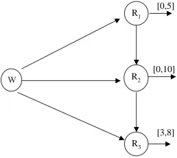
(2004) [14]). Figure 1 displays a warehouse W serving three retailers R1,

R2 and R3. Each retailer faces a demand bounded by a minimum and a

W R2

R₁ [0,5]

[0,10]

[3,8] R3

Fig. 1 Example of one warehouseW and three retailersR1,R2andR3. Retailer

R1 faces a demand in the interval [0,5],R2 in the interval [0,10], andR3 in the

interval [3,8].

[0,5],R2 faces a demandd2 in the interval [d−2, d +

2] = [0,10], andR3 faces

a demandd3in the interval [d−3, d +

3] = [3,8].

After demands di are realized, each retailerRi must choose whether to

fulfill the demand or not. The retailers do not hold any private inventory.

Therefore, if they wish to fulfill their demands, they must reorder goods at

the central warehouse. The retailers may share the total transportation cost

K = 7. Before demands are realized, the warehouse holder decides how to

allocate the transportation costs among the retailers. This decision is only

based on the knowledge of the minimum demandd−_i and maximum demand

d+_i .

The corresponding cost game has a set of three players N ={1,2,3},

namely the three retailers. If player i plays alone, the cost of reordering

coincides with the full transportation cost (since a single truck serves him

only) whereas the cost of not reordering is the cost of unfulfilled demand,

demand. Then the cost associated to the retailersR1andR2are respectively,

c({1})∈£min{d−

1, K},min{d + 1, K}

¤

= [0,5]

c({2})∈£min{d−2, K},min{d+2, K} ¤

= [0,7].

If two players form a coalition they are forced to select a joint decision

(“both reorder” or “both do not reorder”). The cost of reordering for the

coalition also equals the total transportation cost that, this time, must be

shared between the two players. The cost of not reordering is the sum of

the unfulfilled demands of both players. For instance, the cost of coalition

S={1,2}isc({1,2})∈£min{(d−1 +d−2), K},min{(d+1 +d+2), K} ¤

= [0,7].

For a genericn-player game, we have for all coalitions S⊆N

min(K,X

i∈S

d−

i )≤c(S)≤min(K,

X

i∈S

d+_i ). (15)

We can compute the cost savings v(S) of a coalition S as the difference

between the sum of the costs of the coalitions of the individual players inS

and the cost of the coalition itself, namely,

v(S) =X

i∈S

c({i})−c(S). (16)

Given the upper and lower bounds for c(S) in (15), the value v(S) is

bounded as follows:

X

i∈S

min(K, d−_i )−min(K,X

i∈S

d−_i )≤v(S)≤X

i∈S

min(K, d+_i )−min(K,X

i∈S

d+_i ).

For example, the cost savings of coalitionS={1,2}arev({1,2}) =c({1})+

It turns out that the cost savings, or value, of each coalition are bounded

by a minimum and a maximum value, namely, vmin(S)≤v(S)≤vmax(S)

with fixed boundsvmin(S) andvmax(S). Hence, in the light of Definition 1,

an equivalent description of the joint replenishment application is obtained

by replacing the family of cost games by the family of cost-savings games

< N,V >with

V ={v∈Rm:vmin(S)≤v(S)≤vmax(S),for allS ⊆N} (17)

andv(S) as in (16). For the sake of brevity we omit the proof that each game

in the polyhedron (17) corresponds to a balanced game. We conclude that

the joint replenishment problem can be described by the family of balanced

games < N,V >. To see the dynamic aspect of the application, consider

a situation where the discussed scenario occurs repeatedly in time, i.e., at

each time (day, week) k = 0,1, . . ., the warehouse manager allocates the

costs and demands are realized.

3 Dynamic Allocation Rule

The dynamic allocation rule that we propose as a solution to Problem 1

depends on an augmented state variable, to be defined below. Such a state

variable models the excess level of each coalition combined with the

devia-tion of the instantaneous allocadevia-tion from the pre-defined average allocadevia-tion

of each coalition. With the given augmented state variable Problem 1

system. Actually, as it will be clearer later on,ǫ-stabilizing the augmented

system implies bothǫ-stabilizing the excess vector and meeting the average

constraints.

Given two matricesAandD as in (12) and (13), from a standard

prop-erty of linear algebra, see also the appendix, we can find two matrices C

andF that “square”AandD and satisfy

    A C     · D F ¸

=I. (18)

Now, consider the augmented system

x(k+ 1) =x(k) +Au(k)−v(k),

y(k+ 1) =y(k) +Cu(k),

(19)

wherev(k) is as in (6). The additional dynamic variabley(k) keeps track of

the deviation between the instantaneous and the average allocation of each

player. Define the augmented state variablez∈Rn+m−1 as

z(k) =

· D F ¸    

x(k)

y(k)

   ,    

x(k)

y(k)

   =     A C     z(k).

This variable satisfies the equation

z(k+ 1) =

· D F ¸    

x(k+ 1)

y(k+ 1)

    = · D F ¸    

x(k)

y(k)

   + · D F ¸     A C   

 u(k)− · D F ¸    

v(k)

0



  

This indicates that the allocation ruleu(k) =−z(k), which is linear inz,

solves our problem.

Theorem 1Consider system (20) withv(k) as in (6). The allocation rule

in feedback form

u(k) =−z(k) (21)

satisfies

kz(k)k ≤ kDv(k)k. (22)

Further, if the average coalitions’ value is ¯v then the average allocation

vector isu¯.

Proof To prove (22), we substitute the allocation rule (21) in the dynamics

of system (20). This results in z(k+ 1) = −Dv(k) for all k, which

im-plies (22). For the rest of the proof, by summing (20) for different k =

1,2, . . ., we obtain

1 T

T−1 X

k=0

u(k)− 1 T

T−1 X

k=0

Dv(k) =z(T)−z(0)

T →0

asT → ∞, since the numerator is a finite quantity whereas the denominator

tends to infinity. Therefore ¯u=D¯v, which concludes the proof. ⊓⊔

For fixed ǫ we wish to find the maximum time period Θ∗ _{such that}

kDv(k)k ≤ ǫ. Trivially, such a value is Θ∗ ₌ ǫ

δ where δ = maxv∈Vb|Dv|.

Then we have the following corollary.

Corollary 1Consider system (20) withv(k)as in (6). For anyǫand

cor-respondingΘ∗_{, ifΘ≤min{Θ}∗_{,1}, then the allocation rule in feedback form}

isǫ-stabilizing.

Proof It is easy to show that

kz(k)k ≤ kDv(t)Θk ≤ kDv(t)Θ∗k ≤max

v∈Vb

|DvΘ∗| ≤ǫ.

⊓ ⊔

A side effect of kzk ≤ ǫ is that also kuk ≤ ǫ as u = −z. This means

that the smaller ǫ the smaller the maximum allocation (in magnitude).

Also, observe that the above results can be extended to the case where ¯v

is averaged on-line (see Remark 1), with the difference that matrixD must

be updated iteratively according to (12)-(13).

4 Other algorithms in the literature

The idea ofǫ-stabilizing or shrinking the excess vector can be found, from

a different perspective, also in the algorithms proposed by Cesco (1998) [7],

Lehrer (2002) [12] and Sengupta et al.(1996) [16]. Though we have

devel-oped our algorithm independently from the ones cited above, a-posteriori

we recognize that all of them propose an allocation rule that uses a measure

of the extra benefit that a coalition has received up to the current time by

re-distributing the budget among the players. Budget distribution occurs

iteratively until the allocation process converges to an element in the core

or in the ǫ-core if the game is not balanced (in this last case the core is

empty). However, unlike the game in this paper, the games dealt with in [7,

of the coalitions are known and time invariant. Therefore these dynamic

processes refer to allocations of payments to the players and not to the

vari-ation of the coalitions’ values. Owing to the fact that, in this paper, the

values of the coalitions vary unknowingly, we have been able to guarantee

the convergence to the core only in the long run. Furthermore, if we look at

the game < N, v(k)>,ǫ-stabilization implies that the vector of payments

belongs to theǫ-core of the game at each timek= 0,1, . . ..

A last comment regards the computational complexity of the algorithm.

In this sense, it must be noted that to compute the matrixD, upon which the

allocation rule is based, the number of constraints of type (10) to consider

grows exponentially on the number of players n. We refer the reader to

Bausoet al.[4], Section 5, for a procedure based on constraints generation

that returns the matrixD in polynomial time.

5 The Shapley value as a linear allocation rule

In this section we study the Shapley value as a special linear allocation

rule of the form (14). In particular, we show that there is a matrixΦthat

satisfies (12).

The Shapley value φ, introduced in Shapley (1953) [17], is defined by

φ= _n1_!P_σ∈Π(N)mσ _{where Π(N) is the set of all permutations of N and}

mσ _{is the marginal vector corresponding to the permutation σ :N → N.}

A marginal vectormσ _{corresponds to a situation in which the players enter}

receives the marginal contribution he creates upon entering. Hence, mσ _is

the vector inRn with elements

mσ_σ(1) =v({σ(1)}),

mσ

σ(2) =v({σ(1), σ(2)})−v({σ(1)}),

.. .

mσ_σ(k)=v({σ(1), σ(2), . . . , σ(k)})−v({σ(1), σ(2), . . . , σ(k−1)}).

Theorem 2The Shapley value φ is linear in v, i.e., φ = Lv, where the

matrixL∈Rn×m is defined by

Lij=

1 n!·

   

  

−µ!(n−(µ+ 1))! if i6∈S

(µ−1)!(n−µ)! ifi∈S.

(24)

if columnj corresponds to coalition S with µ=|S|.

Proof The proof follows immediately from the definition of the Shapley

value in Shapley (1953) [17]. ⊓⊔

To emphasize the dependence of φ on v we henceforth write φ(v)

in-stead ofφ. Lets(φ(v)) be the vector of surplus variables when revenues are

allocated according to the Shapley valueφ(v). The idea is now to express

s(φ(v)) linearly inv.

Theorem 3The vector of surplus variables is linear inv, i.e.,

s(φ(v)) =Qv, (25)

whereQ∈R(m−1)×m _{has rowi associated to a surplus variable (a coalition}

element

Qij =

   

  

P

p∈SLpj ifi6=j

P

p∈SLpj−1ifi=j.

(26)

Proof First, consider the coalition containing just player 1 and let Li• be

the genericith row ofL. The associated surplus variable is

s1(φ(v)) =φ1−v({1}) =L1•v−v({1}) = (L11−1)v({1})+L12v({2})+. . .+L1mv(N).

The latter equation yieldsQ1•= [(L11−1)L12. . . L1m],which is in

accor-dance with (26).

If we repeat the same reasoning for a generic coalition M ⊂ N, the

surplus variable is

sM(φ(v)) =

X

i∈M

φi−v(M) =

X

i∈M

Li•v−v(M).

Remindjis the column associated to coalitionM. Then, the latter equation

yields Qjk = Pi∈MLik if k 6= j and Qjj = Pi∈MLij −1 which is in

accordance with (26). ⊓⊔

Using the fact thatφ(v) ands(φ(v)) are linear inv, we define the

alloca-tion vector associated to the Shapley value byu(φ(v)) = [φ(v)′ _s(φ(v))′_]′_.

Corollary 2There exists a matrixΦ∈R(n+m−1)×m, defined byΦ= [L′ _Q′_]′

such thatu(φ(v)) =Φv. FurthermoreΦis a right inverse ofA, i.e.,AΦ=I.

Proof From the Theorems 2 and 3 we conclude [φ(v)′ _s(φ(v))′_]′

= [L′ _Q′_]′ v.

This finishes the proof of the first part.

To prove that AΦ=I, it suffices to show that Ai•Φ•j = 1 ifi=j and

is associated to a coalition M ⊆ N, whereas column j of Φ, denoted by

Φ•j ∈R(n+m−1)×1, is associated to a coalitionS⊆N. Hence, the condition

i=j is equivalent toM =S.

Now consider once again the row vector Ai•. The first n elements of

this vector correspond to playersp= 1, . . . , n and the lastm−1 elements

correspond to all coalitionsR ⊂N (recall the structure of A as described

in (2)). Now the structure of rowAi• may be formulated as:

Ai•= [. . . 1

|{z}

∀p∈M

. . . 0

|{z}

∀p6∈M

. . . −1

|{z}

R=M

. . . 0

|{z}

∀R6=M

. . .]. (27)

Analogously, the firstn elements of Φ•j correspond to players p= 1. . . n,

and the lastm−1 elements correspond to all coalitions R ⊂N (see (24)

and (26)).

Concluding, ifi=j, orM =S, thenAi•Φ•j =Pp∈SLpj−(Pp∈SLpj−

1) = 1.On the other hand, ifi6=j, orM 6=S, thenAi•Φ•j =_n1_![P_p∈MLpj−

P

p∈MLpj] = 0. ⊓⊔

6 Conclusions

Inspired by a joint replenishment application, we studied a dynamic

co-operative game where at each point in time the value of each coalition of

players is unknown and fluctuates within a bounded polyhedron. Under the

assumption that the average value of each coalition in the long run is known

with certainty, we have presented a constructive method to find “robust”

allocation rules, i.e., allocation rules that are close to an excess vector and

References

1. S.Z. Alparslan G¨ok, S. Miquel, and S. Tijs,Cooperation under interval

uncer-tainty, CentER DP 2008-09, Tilburg University (to appear in MMOR).

2. S.Z. Alparslan G¨ok, R. Branzei, and S. Tijs,Cores and stable sets for interval

valued games, CentER DP 2008-17, Tilburg University.

3. S.Z. Alparslan G¨ok, R. Branzei, and S. Tijs,Conves interval games, CentER

DP 2008-37, Tilburg University.

4. D. Bauso, F. Blanchini, and R. Pesenti, Robust control strategies for

multi-inventory systems with average flow constraints, Automatica, Special Issue on

Optimal Control Applications to Management Sciences 42, 8 (2006), 1255–

1266.

5. O.N. Bondareva, Some applications of linear programming methods to the

theory of cooperative games, Problemy Kibernet,10(1963), 119–139.

6. N. Cesa-Bianchi, G. Lugosi, G. Stoltz, Regret Minimization Under Partial

Monitoring, Mathematics of Operations Research,31, 3(2006), 562–580.

7. J.C. Cesco,A convergent transfer scheme to the core of a TU-game, Revista

de Matem´aticas Aplicadas,19, 1-2(1998), 23-35.

8. J.A. Filar and L.A. Petrosjan, Dynamic Cooperative Games, International

Game Theory Review2, 1(2000) 47–65.

9. B.C. Hartman, M. Dror, and M. Shaked, Cores of inventory centralization

games, Games and Economic Behaviour31, 1(2000), 26–49.

10. A. Haurie,On some Properties of the Characteristic Function and the Core of

a Multistage Game of Coalitions, IEEE Transactions on Automatic Control

11. L. Kranich, A. Perea, and H. Peters, Core concepts in dynamic TU games,

International Game Theory Review,7(2005), 43–61.

12. E. Lehrer,Allocation Processes in Cooperative Games, International Journal

of Game Theory,31(2002), 341–351.

13. A. Meca, I. Garcia-Jurado, and P. Borm,Cooperation and Competition in

In-ventory Games, Mathematical Methods of Operations Research57, 3(2003),

481–493.

14. A. Meca, J. Timmer, I. Garcia-Jurado, and P. Borm,Inventory games,

Euro-pean Journal of Operational Research156(2004), 127–139.

15. D. Schmeidler,The Nucleolus of a Characteristic Function Game, SIAM

Jour-nal of Applied Mathematics17(1969), 1163–1170.

16. A. Sengupta, K. Sengupta, A property of the core, Games and Economic

Behavior,12(1996), 266-273.

17. L.S. Shapley, A Value for n-Person Games. Contributions to the Theory of

Games II (1953), 193–216.

18. L.S. Shapley,On balanced sets and cores, Naval Research Logistics Quarterly

14(1967), 453–460.

19. J. Suijs and P. Borm,Stochastic Cooperative Games: Superadditivity,

Convex-ity, and Certainty Equivalents, Games and Economic Behavior27, 2(1999),

331–345.

20. J. Suijs, P. Borm, A. De Waegenaere, and S. Tijs, Cooperative games with

stochastic payoffs, European Journal of Operational Research 113 (1999),

193-205.

21. S. Tijs,Introduction to Game Theory, Hindustan Book Agency (2003).

22. J. Timmer, P. Borm, and S. Tijs, On three Shapley-like solutions for

(2003), 595–613.

23. J. Timmer, P. Borm, and S. Tijs, Convexity in stochastic cooperative

situa-tions, International Game Theory Review7(2005), 25–42.

A Computation of the matricesC and F

In this appendix we show how to compute the matrices C and F given

the matricesA andD, as mentioned in Section 3. To simplify notation let

n+m−1 =r. Note that the following conditions follow from (18):AD=I,

AF = 0,CD= 0, andCF =I. First, we rewrite the matricesA, C, D and

F as follows.

– A = [A0 A1 ] where A0 is a m×(r−m) matrix andA1 is an m×m

non singular matrix.

– C = [ C0 C1 ] where C0 is a (r−m)×(r−m) matrix and C1 is an

(r−m)×mmatrix.

– D= [D′

0 D′1]

′

whereD0is an (r−m)×mmatrix andD1 is anm×m

non singular matrix.

– F = [F′

0 F1′]

′

where F0 is a (r−m)×(r−m) matrix and F1 is an

m×(r−m) matrix.

Next, we derive the following relations:

– from AF = 0, we obtainA1F1=−A0F0. SoF1=−A−11A0F0;

– from CD= 0, we obtainC1D1=−C0D0. ThusC1=−C0D0D−11;

– from CF = I, we obtain C0F0 = I−C1F1 = I +C0D0D−11F1 =

Imposing, e.g., C0 = I we have F0 = (I+D0D1−1A−11A0)−1.

Conse-quently,

C= [I | −D0D−11 ]

F =



  

(I+D0D−11A−11A0)−1

−A−1

1 A0(I+D0D1−1A− 1 1 A0)−1

