Rochester Institute of Technology
RIT Scholar Works
Theses
Thesis/Dissertation Collections
12-12-2016
A Methodology to Quantify Cumulative Damage
Function (CDF) for Integration Into an
Object-Oriented Life Cycle Assessment (LCA)
Devdatta Deo
[email protected]Follow this and additional works at:
http://scholarworks.rit.edu/theses
This Thesis is brought to you for free and open access by the Thesis/Dissertation Collections at RIT Scholar Works. It has been accepted for inclusion
in Theses by an authorized administrator of RIT Scholar Works. For more information, please [email protected].
Recommended Citation
R
OCHESTERI
NSTITUTE OFT
ECHNOLOGYA
METHODOLOGY TO QUANTIFYC
UMULATIVED
AMAGEF
UNCTION(CDF)
FORINTEGRATION INTO AN OBJECT
-
ORIENTEDL
IFEC
YCLEA
SSESSMENT(LCA)
FRAMEWORK
By
Devdatta Deo
A Thesis
Submitted in Partial Fulfillment
of the Requirements for the Degree of
Master of Science in Industrial & Systems Engineering
in the
Department of Industrial and Systems Engineering
Kate Gleason College of Engineering
Rochester Institute of Technology
Rochester, NY
December 12, 2016
ii
KATE GLEASON COLLEGE OF ENGINEERING
ROCHESTER INSTITUTE OF TECHNOLOGY
ROCHESTER, NY
CERTIFICATE OF APPROVAL
M.S. DEGREE THESIS
The M.S. Degree thesis of Devdatta Deo
has been examined and approved by the
thesis committee as satisfactory for the
thesis requirements for the
Master of Science degree
Approved by:
Dr. Marcos Esterman, Thesis Advisor
iii
Acknowledgement
I would first like to thank my primary thesis advisor Dr. Marcos Esterman. It would not have been
possible to complete the thesis without his guidance and encouragement. His door was always open
whenever I ran into any problems during the course of the research. I owe my deepest gratitude to him for
the guidance that he provided.
I would also like to thank Dr. Brian Thorn for his feedback and guidance in the area of Life cycle
assessment.
I would like to acknowledge the Industrial & Systems Engineering department at RIT for the financial
support without which it would have been impossible for me to purse the Master’s degree.
Last but not the least, I would like thank my parents, sister and my brother in law for their love and
iv
Abstract
Life Cycle Assessment (LCA) is one of the most widely used tools to determine the environmental impact
of products and processes. One of the main concerns with LCA is the limited comparability of the results
due to limitations in defining the functional unit. This affects goal and scope definition of the LCA
studies. A result, an object-oriented framework for LCA that integrates functional analysis and systems
engineering principles was developed. In this research a cumulative damage function (CDF) to quantify
the life of components, subsystems and components was defined. However, the development of the
methodology and underlying principles to develop the CDF was left for future work. The purpose of this
thesis is to develop a framework to quantify CDF using the concepts of Remaining Useful Life (RUL),
reliability analysis and failure analysis so that it can be easily integrated into the object-oriented LCA
framework. This thesis will present a 5-step methodology to quantify the CDF and demonstrate its use
and effectiveness by implementing it on a manual can opener and a coffee maker as examples of product
v
Contents
1. Background ... 1
1.1 Life Cycle Assessment ... 1
1.2 Cumulative Damage Function ... 4
2. Literature Review ... 6
2.1 Reliability ... 6
2.2 Remaining Useful Life ... 7
3. Problem Statement ... 16
3.1Clarification of the Problem... 16
3.2 Research Objectives ... 19
4. Framework Development ... 21
4.1 Methodology to develop a framework to calculate Cumulative Damage Function ... 21
4.2 Example ... 30
Alternate method to compute CDF ... 44
5. Case study ... 46
5.1 Introduction ... 46
5.1.1 Theory of operation ... 46
5.1.2 Coffee brewing ... 47
5.2 Application of framework ... 48
6. Conclusion and Future work ... 68
Bibliography ... 70
Appendix A ... 74
Appendix B ... 83
vi
Table 2: FMECA can opener ... 38
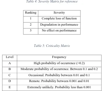
Table 3: Criticality Matrix ... 38
Table 4: Severity Matrix for reference ... 39
Table 5: Criticality Matrix ... 39
Table 6: Inputs to functional decomposition ... 49
Table 7: Identified Sub-functions in the Keurig Product System ... 55
Table 8: Average use scenario for coffee consumption... 58
Table 9: User parameters and Sub-functions ... 59
Table 10: DSM level 1 ... 60
Table 11: DSM level 2 ... 60
Table 12: DSM level 3 ... 62
Table 13: Critical Failure in Prepare S+C ... 63
Table 14: FMECA with critical failure ... 65
Figure 1: Life Cycle Stages ... 1
Figure 2: Typical Bathtub Curve (adapted from (Bernd, 2008)) ... 7
Figure 3: RUL Classification ... 8
Figure 4: Remaining Useful Life ... 19
Figure 5: System reference of CDF ... 22
Figure 6: Methodology to compute CDF ... 25
Figure 7: Functional Decomposition ... 28
Figure 8: Can Opener ... 30
Figure 9: Primary Function of can opener ... 31
Figure 10: Functional decomposition of Can opener ... 32
Figure 11: Functional Decomposition with CDF ... 44
Figure 12: Keurig system overview (Keurig use & care guide K2.0 series, 2015) ... 47
Figure 13: Primary function of Keurig ... 49
Figure 14: First level functional decomposition ... 50
Figure 15: Decomposition of Extract Soluble ... 51
vii
Figure 17: Prepare S+C functional decomposition ... 52
Figure 18: Feature based decomposition ... 53
Figure 19: Prepare Water functional decomposition ... 54
Figure 20: Transfer soluble functional decomposition ... 54
Figure 21: Prepare S+C functional decomposition ... 56
Figure 22: Functional Analysis of heat water ... 56
Figure 23: Functional decomposition of Transfer Soluble to Water ... 57
1
1
.
Background
1.1 Life Cycle Assessment
Environmental awareness at many companies has increased and they have responded by developing
environmentally friendly products and incorporating ecofriendly processes. These companies assess the
impact of their products and processes on the environment in an attempt to minimize these impacts and
one of the tools widely used by companies for environmental assessment is Life Cycle Assessment
(Curran 2006).
Life Cycle Assessment ‘studies the environmental aspects and potential impacts throughout a product’s
life (i.e. cradle-to-grave) from raw material acquisition through production, use and disposal (see Figure
1). The general categories of environmental impacts needing consideration include resource use, human
health, and ecological consequences (ISO 14040 2006). Curran (2006) highlighted some of the strengths
of the Life Cycle Assessment framework which include:
1. It is a comprehensive assessment tool
2. Highlights potential trade offs
3. Provides a structure to the investigation
4. Can challenge conventional wisdom
5. Advances the knowledge base
6. Fosters communication and disclosure
RAW MATERIAL ACQUISITION
RAW MATERIAL
[image:9.612.79.534.402.655.2]ACQUISITION MANUFACTURINGMANUFACTURING USE/MAINTENANCEUSE/MAINTENANCE RECYCLERECYCLE END OF LIFEEND OF LIFE
Figure 1: Life Cycle Stages
Life Cycle Assessment framework, as defined by the ISO framework is given below (ISO 14040 2006)
2
1. Goal Definition and Scoping - Define and describe the product, process or activity. Establish the
context in which the assessment is to be made and identify the boundaries and environmental
effects to be reviewed for the assessment.
2. Inventory Analysis - Identify and quantify energy, water and materials usage and environmental
releases (e.g., air emissions, solid waste disposal, waste water discharges).
3. Impact Assessment - Assess the potential human and ecological effects of energy, water, and
material usage and the environmental releases identified in the inventory analysis.
4. Interpretation - Evaluate the results of the inventory analysis and impact assessment to select the
preferred product, process or service with a clear understanding of the uncertainty and the
assumptions used to generate the results.
Another important aspect of LCA is that it is considered to be relative in nature since the assessment is
based on a functional unit and results are presented in a comparative way (ISO 14040 2006). The standard
states that the primary purpose of a functional unit is to provide a reference, and, therefore ensure
comparability of LCA results. However, as shown by (Fumagalli, et al., 2012) comparing LCA studies is
difficult due to the lack of standardized assumptions and practices including the definition of functional
unit. In their work, they have proposed a method to integrate systems engineering and functional analysis
concepts to the goal and scope definition of Life Cycle Assessment phase to define the system, system
boundary and reference flows. The advantage of the method developed by (Fumagalli et al. 2012)
includes improved comparability of LCA, dynamic updating of LCA and its integration with early stage
product development.
Fumagalli (2012) describes various issues related to LCA and states that the functional unit definition and
boundary selection are one of the most critical issues in the early stages of LCA as they form the base of
the study. This same work further highlights that the current ISO norms do not provide any guidance in
defining the functional unit which results in large variability in the LCA studies and hence difficulty in
3
As a response, Fumagalli (2012) proposed the use of functional modelling as a powerful tool to
functionally decompose a product in order to understand the product in an abstract manner without the
need to define the product structure. According to Stone & Wood (2000) a function is represented as a
verb-object pair where the object represents the reference flow. There are three types of reference flows
considered in the functional decomposition namely, material flow, energy flow and information flow. ISO
14040 identifies the importance of defining the flows to ensure comparability of LCA’s(ISO 14040,
2006). Fumagalli (2012) points out that the identification of the reference flows establishes the link
between LCA and functional analysis. The initial feasibility of this approach was illustrated through
examples using black box model abstractions of classes of systems (Fumagalli 2012). One of the
advantages of this approach is that the user behavior is external to the system thus decoupling the use
behavior and functional unit which will lead to a structured approach to develop LCA.
One of the issues that arose while implementing the framework described above, was related to the
allocation of reference flows during the inventory phase of the LCA. This resulted in defining of a
Cumulative Damage Function (CDF), which represents the usage profile and wear of the system under
study and depends on the use variables (Fumagalli 2012). Thus CDF is an important concept which helps
to establish the relationship between LCA and functional analysis in order to establish the proper
allocation of the flows. It is important that the reference flows (which represent the material and energy
transformations in the system) that are identified are abstract enough so that they are independent of the
system architecture and that they can be scaled relative to the user behavior (Fumagalli 2012).
As previously stated, one of the important contributions of the framework described above was to
decouple user behavior from the definition of the functional unit. The advantage of defining use phase
boundaries, reference flows and scalable parameters is that it will enable the development of an
object-oriented LCA framework. However, an important supporting concept is that of CDF which was not fully
developed in the aforementioned framework. In the following section, the concept of CDF is described
4
1.2 Cumulative Damage Function
The Cumulative Damage Function is a function of usage parameters and it represents portion of the ‘life’
of a product, subsystem or product that is consumed based on these usage parameters (Fumagalli 2012).
The CDF is ultimately based on the technology employed to implement the system and the system
architecture. The form of this function can be established by using various traditional tests like
accelerated life tests, endurance tests, and reliability tests. The input parameters for the CDF are the user
parameters which are developed based on the functional analysis of the system. This helps to ensure that
these user parameters are independent of the technology used for implementation, which enables better
comparability of the LCA results.
The CDF is used to relate the use scenarios with the consumed life of the product and can be used to
calculate the life cycle inventory based on the reference flows identified in the functional decomposition.
One of the advantages of having a CDF is that it can be used for comparing different technologies used
for implementing same function. It can be used to identify all of the workflows associated with the given
system.
The CDF is mathematically defined as:
𝐶𝐷𝐹 = 𝐶𝑜𝑛𝑠𝑢𝑚𝑒𝑑 𝑙𝑖𝑓𝑒
𝐿𝑖𝑚𝑖𝑡(𝐿𝑓, 𝐿𝑜𝑏𝑠, 𝐿𝑛𝑒𝑒𝑑)
(1)
𝐶𝐷𝐹: 𝐴𝑚𝑜𝑢𝑛𝑡 𝑜𝑓 𝐵𝑂𝑀 𝑡𝑜 𝑏𝑒 𝑞𝑢𝑎𝑛𝑡𝑖𝑓𝑖𝑒𝑑 𝑓𝑜𝑟 𝐿𝐶𝐴
𝐶𝑜𝑛𝑠𝑢𝑚𝑒𝑑 𝑙𝑖𝑓𝑒: 𝑏𝑎𝑠𝑒𝑑 𝑜𝑛 𝑡ℎ𝑒 𝑢𝑠𝑒𝑟 𝑠𝑐𝑒𝑛𝑎𝑟𝑖𝑜
𝐿𝑓: 𝐿𝑖𝑚𝑖𝑡 𝑑𝑢𝑒 𝑡𝑜 𝑓𝑎𝑖𝑙𝑢𝑟𝑒
𝐿𝑜𝑏𝑠: 𝐿𝑖𝑚𝑖𝑡 𝑑𝑢𝑒 𝑡𝑜 𝑜𝑏𝑠𝑜𝑙𝑒𝑐𝑒𝑛𝑠𝑒
𝐿𝑛𝑒𝑒𝑑: 𝐿𝑖𝑚𝑖𝑡 𝑑𝑢𝑒 𝑡𝑜 𝑙𝑎𝑐𝑘 𝑜𝑓 𝑛𝑒𝑒𝑑 𝑜𝑓 𝑡ℎ𝑒 𝑝𝑟𝑜𝑑𝑢𝑐𝑡
In this function, numerator represents the amount of life consumed for the given system and it depends on
the user behavior, usage environment etc. The denominator represents the limit of the product/system
5
a failure in the product, obsolescence of the technology in use or simply that there is no need of the
product anymore. Thus the CDF represents the amount of bill of material to be quantified for the
inventory phase of the LCA for the given user scenarios.
While the work described above illustrated the concept of CDF through an example, the rigorous
definition of the CDF was left for future work (Fumagalli 2012).In addition, problems associated with
developing the CDF are not discussed nor are the limitations associated with its use. Thus there is a need
to develop a framework and guidelines to standardize the development and the use of the CDF so that it
can be integrated with the object-oriented LCA framework. In this thesis, a standardized framework to
calculate the cumulative damage function will be developed. In addition, its integration into an
objected-oriented framework will be illustrated though a detailed case study.
The remainder of this thesis is organized in the following manner: Chapter 2 will present the literature
review which will describe related concepts that will help to develop the CDF framework described in
this thesis. Chapter 3 will formally define the thesis goals and objectives. Chapter 4 will describe the
development of the framework. Chapter 5 will illustrate the framework on a detailed product example.
6
2. Literature Review
Literature Review
This chapter will review the literature on the integration of reliability modelling with Life Cycle
Assessment, functional analysis techniques and the concepts of Remaining Useful Life, including its
application in the fields of remanufacturing and electronics.
2.1 Reliability
Reliability is defined as the probability that a product will operate or a service will be provided properly
for a specified period of time (design life) under the designed operating conditions (such as
temperature, load, volt ) without failure(Elsayed 2012).
Some of the fundamental concepts in reliability are related to failure rates, failure density functions and
the reliability survival functions. The relationship between these three functions is given by the following
equation;
𝜆(𝑡) =𝑓(𝑡)
𝑅(𝑡) (2)
Where 𝜆(𝑡) is the failure rate
f(t) is the number of failures
R(t) is the survival probability
t is time
The failure rate can be interpreted as a measure of the risk that the part will fail if it has survived to up
until time t. The failure rate always results in the characteristics curve which resembles a bath tub curve
(Bernd 2008). A typical bathtub curve is shown in Figure 2. The bathtub curve shown below is divided in
three regions: the first part is related to early failures where failure rate is high but reducing; in the middle
section the failure rate stabilizes, this region is called random failures; and finally in the wear out region
7
impact on the remaining useful life of the product. As the region in which the product is being operated
can introduce some uncertainty in the RUL calculations, however for this phase of the research,
[image:15.612.107.515.179.400.2]uncertainty is not being considered
Figure 2: Typical Bathtub Curve (adapted from (Bernd, 2008))
Reliability analysis can also be carried out either quantitatively or qualitatively. According to (Bernd
2008), the Weibull distribution is the most commonly used lifetime distribution to determine the
reliability of the products.
2.2 Remaining Useful Life
Remaining useful life (RUL) is the useful life left on an asset at a particular time of operation. RUL is
generally random and unknown and must be estimated from the information that is collected using
prognostics and health management. Recently, due to increased emphasis on the cost of maintenance and
product replacement, greater emphasis has been put on estimating the RUL of the system so that
8
estimate for remaining useful life but several different statistical and physics of failure based methods
have been developed to support different types of products. Statistical data-driven models are appropriate
when the physical laws of the system in operation are not known. The classical data-driven models
include the use of stochastic models such as the autoregressive (AR) model and the multivariate adaptive
regression splines. Recently, there has been more interest in neural networks (NNs) and neural fuzzy (NF)
systems have been developed. Different Dynamic Bayesian networks models have also been used for
prognostics.(Mosallam et al., 2013).
(Sikorska et al., 2011) have classified RUL prediction methodologies into knowledge based models, life
expectancy models, artificial neural network models and physical models as shown in Figure 3 (adapted
from Sikorska et al., (2011). As one moves from the knowledge based models to physical models the
complexity of the models increase. Knowledge based models can be further classified into fixed or fuzzy
models. Life expectancy models can be further classified into stochastic models, which are further
classified into Bayesian network models, Markov models, hidden Markov models, Kalman filters and
particle filters. Life expectancy models are further classified into Statistical models which could be
prognostics and health management models or regression models.
Remaining
Useful life
Model Based
Knowledge
Based
Analytical
Based
Hybrid Based
9
A systematic review of the literature on methods to estimate the RUL of assets showed that the RUL of
an asset depends on the current age of the asset, the operating environment and the observed condition
monitoring or the health information (X. S. Si et al., 2011). Mathematically, Xt is the random variable for
RUL at time t, then the PDF of Xt, is dependent on Yt, which is the operational history of the system.
Thus, 𝑓(𝑋𝑡|𝑌𝑡) is the RUL unless Yt is not known and then RUL is simply F(Xt+t)/R (t), where R(t) is
the survival probability based on the failure rate(X. S. Si et al., 2011).
The statistical data based approaches mentioned before determine the RUL by fitting data to the model
without considering the underlying physical models for failure. In order to use statistical models there are
two types of data sets available. The first type is the event data associated with the failure data and the
condition monitoring data, which is a real-time monitoring of the asset under use for any changes in the
operational conditions and parameters. According to RUL, statistical models are classified into two
categories, those based on direct state monitoring and those which rely on indirect state monitoring.
Regression, Wiener and Gamma based processes are continuous processes while Markovian models are
based on the discrete processes. These process will not be discussed in detail here but these processes are
discussed in (X. S. Si, et al., 2011). (X. S. Si, et al., 2011) give a general overview of various statistical
approaches available to estimate RUL. However, there are several other approaches which can be used to
estimate the RUL, based on factors such as the applications or the product itself.
Classification of RUL methodologies has also been done on the basis of the application industry
(Sikorska et al., 2011). (Sikorska et al., 2011) discuss the pros and cons of various methodologies
including Artificial Neural networks as an approach for determining the RUL. Artificial Neural Networks
(ANN) compute an estimated output for the RUL of the component from a mathematical representation of
the system derived from the observed data. These methods are very useful for non-linear processes.
According to (Sikorska et al. 2011) there are two types of networks, either feed forward or dynamic
networks and both can be used to calculate the RUL. Feed forward networks are also known as static
10
have some knowledge of the actual system. One of the limitations of using ANN is that it requires an
extensive training data set to train the network and this means that accurate results for the training data
sets need to be available so that the synaptic weights can be assigned to the networks so that the network
can be used to estimate the RUL in the future. Constructing an appropriate model is a trial and error
approach and requires extensive data and time.(Sikorska et al., 2011).
Another approach used widely to calculate the RUL is to use degradation data. One of the methods
developed by (X.-S. Si et al. 2012) is based on non-linearity in the degradation process. This process
gives better results in terms of the accuracy of the RUL. A key idea behind this approach is that the
lifetime can be defined as the First Hitting Time (FHT) of the degradation process reaching the threshold
value (beyond which the system fails) and the PDF of RUL is modelled as a PDF of the FHT. But there is
no closed form solution for non-linear degradation processes and hence an analytical approximation is
developed for the distribution of FHT. Parameters for the degradation process are estimated using a
Maximum Likelihood Estimator and goodness of fit testing is used to determine the model fit. This model
gives a better fit if the degradation process is non-linear.
Another approach developed by Su & Jiang (2009) also uses degradation data to calculate RUL. They use
degradation amplitude to model the product life. Based on the degradation amplitude size different
distributions can be fit and goodness of fit is used to determine the appropriate distribution. This
methodology is applied to GaAs (Gallium Arsenide) Laser to determine the usefulness of this method.
This method is similar to determining the MTTF using a Weibull or Gaussian distribution. This method
may be useful to determine the CDF, but a problem may be faced when collecting the degradation data.
There are some other approaches which can be used to calculate the RUL. For example, a Bayesian
approach is widely used to calculate RUL (Mosallam et al., 2013). In (Mosallam et al., 2013), an
approach for data driven prognostics is presented. The approach starts by building an offline trends
database extracted from multidimensional datasets. These trends are later grouped according to their EOL
11
may be better suited to the objectives of this thesis, however, this method does not consider the
environmental conditions in which the products operate. This method may not be suitable to develop a
simulation model to calculate the RUL to develop a CDF.
In addition to the methods discussed above there are several approaches, which have been developed
based on the product or applications. One such approach is considered by (Okoh et al, 2014) in which the
prediction of catastrophic failure events plays a critical role through the life of engineering services and
RUL is used to predict the life span of the product to prevent such a catastrophic event. According to the
authors, RUL models can be classified as;
(Okoh et al, 2014) focus on RUL techniques for gas turbine components. They identify various
degradation mechanisms and then map them with corresponding RUL techniques to identify appropriate
RUL methods. The authors identify wear, corrosion, deformation and fracture as important degradation
mechanisms in gas turbines. The important degradation mechanisms present in the product are mapped to
suitable RUL methods but no specific methods to calculate RUL are developed. They do suggest a
methodology for prognostics and health management.
Another approach is developed by Mathew et al. (2008) for the prognostics of electronic products is based
on Failure Modes, Mechanisms and Effects Analysis (FMMEA). However, in order to implement this
method it is necessary that the users know the underlying failure modes and models of the product in
order to develop the canary devices (i.e. early warning systems) which give the precursor information of
the failure. This approach is similar to the one developed by Okoh et al. (2014). This work also does not
consider the life cycle environment of the products.
Smith et al., (2002) do consider the life-cycle environment by life cycle consumption monitoring of the
product. A recorder is used to monitor temperature, shocks, and vibrations on a printed circuit board
placed in the car engine. This data is then compared to the physics of failure model in order to determine
the damage accumulation in solder joints due to temperature and vibration loads. The RUL of the solder
12
Palmgren-Miners rule the accumulated damage is calculated. In this paper, Physics of Failure models are
used to calculate the number of cycles to failure under the given operating conditions. Based on the
actually accumulated damage calculated from the Miners equation, remaining useful life can be
estimated. This approach, though developed for electronic products can be used on any other system.
However, there is a need to know the underlying failure modes in order to determine the threshold levels
(beyond which the systems fail) to calculate the RUL for the system.
There are some RUL approaches that have been developed for the product take back decisions. One such
approach is developed by Vichare et al. (2004). They use life consumption of the products to determine
the product take back decisions. Life Cycle Monitoring (LCM) is a method of monitoring parameters
indicative of the systems life cycle health and it converts the collected data into an estimate of the life
consumed. This involves continuous monitoring of the product and integrating it with Physics of Failure
models to determine the life consumed. The approach developed by the authors is similar to the one
developed by Smith et al. (2002) but on a different application.
Le Son et al. (2013) developed an approach using Wiener processes combined with principal component
analysis to estimate the RUL. The advantages of using this approach are that it is a probabilistic approach
and it gives better indication of degradation. However, this method may be overly complicated for what
the goals of this thesis are.
In addition to works discussed so far, there is some research where the concept of the RUL is used to
determine the optimal life time products for take back, remanufacture and recycling. Kara et al. (2008)
developed a methodology to determine the products useful life during the design stage itself using product
failure mechanisms and their associated critical lifetime prediction parameters. Their objective was to
develop a methodology which would help to assess product useful life, which in turn would help to
develop sustainable products as this would minimize resource consumption based on the end of life
strategy. Their approach entailed: (1) Clustering products in groups based on their failure mechanisms
13
Assessing products based on the design parameters and expected design life. The methodology was
applied to six different electric motors and a gear box. Initially data was collected for the failure
percentages of each component from an engineering company. Based on this data, products were
clustered in groups using Group Technology and Hierarchical Clustering. After the critical design
parameters for each component were identified, the time to failure data for the electric motors and the
gearbox were collected by observing number of failure per year. These observations were used to develop
lifetime prediction equations using linear regression analysis. However the drawback of this method is
that it is necessary to have a large initial data set. A similar methodology was developed by Kara et al.
(2005) to determine the reuse potential of products.
Rugrungruang et al. (2007) deals with product reuse based on technology and product lifecycles. The
remaining physical life of the product is calculated as a difference between the physical life of the product
and the usage life of the product. The physical life of the product is calculated from MTTF of the product.
The usage life of the product is calculated based on the usage intensity of the product. Using a usage
survey, data is collected from users, which is statistically analyzed to determine frequency and duration
that the product (in this case a Television) spends in active mode. Simulation models are then used to
determine the MTTF of the products.One of the drawbacks of this approach is the failure to consider the
usage environment and various user parameters to calculate the usage of the product.
Based on the literature review, it is reasonable to conclude that the RUL methods available are based on
degradation mechanisms, condition monitoring, and statistical analysis. However, some of these methods
may not be as useful as the amount of data available may be limited, and extensive testing of the products
may not be feasible. Some of the methods that have been reviewed have very specific applications, like
electronic products. Most of the methods that have been reviewed require extensive data and are also
fairly complicated to implement. The following summarizes the main conclusions from the literature
14
1. RUL consists of two main parts data acquisition and data analysis.
2. Data analysis can be based on any of the following methods
a. Trending and degradation curves
b. Covariate models
c. Space state methods ( Markov chains, gamma based state space models)
d. Artificial intelligence
3. Data monitoring can be based on the multiple sensors that are embedded in the product which
continuously gather the data. Various parameters that can be monitored are:
a. Vibration monitoring
b. Acoustic monitoring
c. Acoustic emission and ultrasonic monitoring
d. Oil and wear debris monitoring
e. Ferrography monitoring
f. Thermography monitoring
g. Environmental data analysis
h. Process parameter
4. Various conditional parameters that could be monitored are:
a. Fatigue
b. Wear
c. Deterioration
d. Creep
e. Reliability of components
f. Environmental factors
g. Corrosion
15
5. Once the condition variables are analyzed model based, feature based or hybrid models can be
used to relate the degradation signals to remaining useful life of the system.
6. Approaches for calculating consumed life of a product include;
a. Identify all the components that help achieve a particular user parameter
b. Identify impact on each component in terms of wear, stress, load, fatigue, creep etc.
c. Develop a function to represent this impact over the product
No work that integrated reliability modelling with life cycle assessment to determine the life of the
product was found in the literature review. The next chapter defines the problem based on the initial
16
3. Problem Statement
3.1
Clarification of the Problem
According to ISO 14040 the functional unit is defined as the quantified performance of a product system
for use as a reference unit in a life cycle assessment study. The functional unit is used in Life cycle
assessment studies to ensure that there is comparability between the results of LCA studies. But as
pointed out by various researchers the lack of standardized practices to define functional units, variability
in assumptions, and the lack of guidelines for defining functional unit affect the results of LCA as this
forms the base of any study (Bousquin et al., 2011; Collado-Ruiz & Ostad-Ahmad-Ghorabi, 2010b; Reap
et al., 2008).
In order to overcome this problem, a novel approach was developed by (Fumagalli 2012) to integrate
systems engineering principles and functional analysis into the definition of the goal and scope of a life
cycle assessment. The proposed methodology includes:
1. Define the enclosing system
2. Define reference flows and scaling parameters
3. Separating the functional unit definition from user behavior and developing and using cumulative
damage functions to determine the used life of the product and product components.
The advantage of the proposed method is that it enables the comparison of LCA results conducted on
different products that satisfy similar functions. This is enabled in part by separating user behavior from
the definition of the functional unit. However, the most important part of this framework is that the
reference flows and scaling parameters identified can be modified based on the user scenarios directly or
indirectly. This linkage is achieved by using cumulative damage functions which are defined as a function
of usage parameters. Based on the usage parameters a certain portion of the useful life of the product and
its components will be consumed. The Cumulative Damage Function (CDF) will be dependent on the
17
𝐶𝐷𝐹 = 𝐶𝑜𝑛𝑠𝑢𝑚𝑒𝑑 𝑙𝑖𝑓𝑒
𝐿𝑖𝑚𝑖𝑡(𝐿𝑓, 𝐿𝑜𝑏𝑠, 𝐿𝑛𝑒𝑒𝑑)
(3)
𝐶𝐷𝐹: 𝐴𝑚𝑜𝑢𝑛𝑡 𝑜𝑓 𝐵𝑂𝑀 𝑡𝑜 𝑏𝑒 𝑞𝑢𝑎𝑛𝑡𝑖𝑓𝑖𝑒𝑑 𝑓𝑜𝑟 𝐿𝐶𝐴
𝐶𝑜𝑛𝑠𝑢𝑚𝑒𝑑 𝑙𝑖𝑓𝑒: 𝑏𝑎𝑠𝑒𝑑 𝑜𝑛 𝑡ℎ𝑒 𝑢𝑠𝑒𝑟 𝑠𝑐𝑒𝑛𝑎𝑟𝑖𝑜
𝐿𝑓: 𝐿𝑖𝑚𝑖𝑡 𝑑𝑢𝑒 𝑡𝑜 𝑓𝑎𝑖𝑙𝑢𝑟𝑒
𝐿𝑜𝑏𝑠: 𝐿𝑖𝑚𝑖𝑡 𝑑𝑢𝑒 𝑡𝑜 𝑜𝑏𝑠𝑜𝑙𝑒𝑐𝑒𝑛𝑠𝑒
𝐿𝑛𝑒𝑒𝑑: 𝐿𝑖𝑚𝑖𝑡 𝑑𝑢𝑒 𝑡𝑜 𝑙𝑎𝑐𝑘 𝑜𝑓 𝑛𝑒𝑒𝑑 𝑜𝑓 𝑡ℎ𝑒 𝑝𝑟𝑜𝑑𝑢𝑐𝑡
The purpose of this thesis is to integrate the principles of reliability engineering with Life Cycle
Assessment to support the development of an object-oriented approach for Life Cycle Assessment. As
was discussed above, while Fumagalli (2012) motivated the need and use of the CDF, its rigorous
development was left for future work. In the following paragraphs, the needs to have to be satisfied by
this integration effort will be discussed, which will be followed by a summary of the research objectives.
The CDF quantifies the amount of product or component life that is ‘consumed’ with respect to the total
available life of the product, which is the denominator in the above equation. This definition of CDF
widens the scope of the problem as consumed life cannot only be defined by physical consumption
mechanisms (the most common approach) but also with concepts like perceived obsolescence of the
product which can also limit the life of the system under study, which further complicates the estimation.
Another dimension of complexity is added to the problem as the use of the product under study would be
uncertain which in turn affects the variability of consumed life estimation of the product and affects the
variability of the life cycle inventory calculations. Thus it is necessary to model this uncertainty in the
proposed model.
From the review of the literature, it is clear that there are a variety of different statistical and physical
approaches available to determine the consumed life of the product or component under investigation.
These approaches range from the physical testing of the product under defined test conditions to using
18
also been used in preventive maintenance, prognostics and health management of complex mechanical
systems. However, there is a need to examine the suitability of applying these to define the CDF.
In addition to defining the CDF, it is also necessary to establish the limit of the product under study. Thus
a need exists to deal with the various methods that could be used to establish the limit of the system under
study. Various technology growth forecasting models, substitution models are available which can be
used to establish the limit of the product in terms of technology obsolescence. Various approaches can be
considered to develop guidelines to establish the product limit.
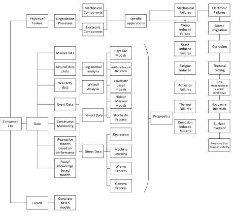
Figure 4 shown below is a representation of the available methodologies to develop an approach to
estimate the remaining useful life of the product. These methodologies will be examined in greater detail
19 Consumed Life Physics of Failure Data Fusion Degradation Processes Mechanical Components Electronic Components Continuous Monitoring Event Data Regression models based on performance Indirect Data Direct Data Regression Machine Learning Wiener Process Gamma Process Covariate based models Hidden Markov Models Stochastic Process Artificial Neural Networks Bayesian Models Log-normal analysis Weibull Analysis Covariate based models Mechanical Failures Creep Induced Failure Crack Induced Failures Fatigue Induced Adhesion Failures Thermal Failures Corrosion induced failures Electronic Failures Stress migration Corrosion Thermal cycling Time dependent di electric breakdown Hot carrier injection Surface inversion Negative bias temp instability Warranty data Acturial data plots Market data Prognostics Fuzzy/ knowledge based models Specific applications
Figure 4: Remaining Useful Life
3.2 Research Objectives
The objective of this thesis is to develop a framework and methodology to quantify the cumulative
damage function based on the user parameters.
Thus the research objectives include:
Assimilate the literature on condition based maintenance, remaining useful life and prognostics
20
Extend the concept of CDF to a functional decomposition to support the development of a
framework for object-oriented life cycle assessments.
Develop rules to integrate CDFs within the functional decomposition to quantify the system level
CDF.
Develop a framework to link system level parameters with use parameters.
Develop a framework to model various user scenarios to assess life cycle impacts.
Propose a method to identify the life limit of the product.
Apply the proposed methodology to a product case study.
In addition to these research objectives, some of the questions that this work will attempt to answer
include:
What is a cumulative damage function? How is it defined in terms of life cycle assessment?
What are the advantages and limitations of CDF in terms of an object-oriented LCA?
21
4. Framework Development
In this section, the framework to estimate the CDF will be developed. This will be done in two sections.
In section 4.1 the methodology to develop the framework will be defined and in section 4.2 the execution
of the methodology will be summarized.
4.1 Methodology to develop a framework to calculate Cumulative Damage Function
The stated objective of this thesis is to support the development of an object-oriented framework for LCA
by developing a framework to calculate the CDF that takes into consideration an object structure that is
derived from the functional breakdown of the main function that a product system fulfills. In order to
accomplish this it is necessary to establish a relation between the user parameters, the reference flows of
the system and the system parameters. This relationship will help to define and keep track of the
consumed life of the product and its components (or objects). Since these CDFs will ultimately be related
to the technology employed to implement the function under consideration it is necessary to consider
specific interactions to establish a correlation between reference flows and user parameters. Note that if
the abstractions that were defined by Fumagalli (2012) are adhered to both the reference flows and the
user parameters will be independent of the specific technology used to implement the functions.
However, the specific CDF will not be independent of the technology. As long as the CDF is a function
of these parameters and the use and flow parameters, the independence between layers of abstraction can
be maintained. Recall that in Fumagalli’s (2012) work that a function is characterized by a minimal set of
reference flows (energy and material) which can be scaled based on the user parameters through the use
of system level parameters. Please note that these reference flows should not be confused with the
reference flows defined by ISO 14040 (ISO 14040 2012; Curran 2006).
In addition to the reference flows (material, energy & information) it will also be necessary to identify the
stressors that affect the reliability of each function. As a matter of fact, the stressors can be considered as
the fourth flow. Figure 5 shows a functional decomposition with identified reference flows. The
22
is further decomposed into sub-functions which integrate to perform the primary function. The main
objective of developing a functional decomposition is to generate a functional abstraction that develops
the product architecture in a controlled manner such that the various degrees of solution independence are
maintained. This will lead black boxes at different abstraction levels connected to each other which is
known as hierarchical function structure (Gadre 2016). As an example consider the decomposition to a
low-level function such as ‘convert electrical energy into rotational energy’. Clearly, the architectural
decision has been made to implement a motor. However, what motor technology is used (e.g. AC or DC)
is still open. In a similar manner, various levels of abstraction and detail can be represented in the
functional hierarchy.
Function
Energy Material
Energy Material
` Interaction
parameters Usage Parameters
Function1 Function2
Function1_1 Function1_2 Function2_1 Function2_2
Material
Energy
Component 1
System level parameters
CDF Consumed
life Material
Energy
Component 1
System level parameters
Combine CDF to obtain system level CDF
[image:30.612.138.480.365.606.2]Consumed life
23
However, one of the difficulties that is anticipated with the identification of the operational stressors is the
fact that these stressors will be related to the system architecture and its evolution as the product/system
design details are decided upon. It is hypothesized that the tops-down functional decomposition proposed
above will allow all of the stressors within the system to be identified based on the information available
at any particular level of functional abstraction. These stressors will be in the form of:
a. Fatigue
b. Wear
c. Deterioration
d. Creep
e. Reliability of components
f. Environmental factors
g. Corrosion
h. Electrical stress
Once consumed and the life for each sub-function is established, it will be necessary to integrate each of
the individual CDFs to develop a CDF for the function that the sub-functions integrate into. The use of
reliability block diagrams or FMEA will be explored as ways to achieve this integration into a function. In
order to test the feasibility of this approach a simple example and a more realistic product example will be
used to develop insights into a framework to calculate the CDF.
The main idea behind the more realistic product example is to develop a functional breakdown of a coffee
maker to identify all of the related reference flows and system parameters associated with all of the
functions that make up the functional hierarchy. This will help to illustrate the concepts developed in this
thesis and to identify implementation issues. Note that the upper level functions of the hierarchy will be
independent of any particular technology for making coffee maker, but as the functions are decomposed
they will necessarily converge to the specific technologies and components utilized in the specific product
24
framework will be applied to these low-level interactions and the proposed method to calculate CDF and
integrate them up the functional hierarchy will be illustrated and resulting LCA of the product will be
developed.
In addition to the issues related to integrating functional analysis with the methodology to compute CDF
to integrate it into an object-oriented LCA framework, the methodology has to ensure integration with
reliability modelling to compute the CDFs. Determining the end of life of the product is one of the issues
that needs to be resolved in order to ensure the calculation of the CDF. This involves understanding the
various mechanisms under which products become obsolete, for example, due to the arrival of some new
technology. Daimon and Kondoh (2003) state that the main reasons for product obsolescence arise from
either physical causes or value causes. Physical causes could be due to the consumption of function or due
to a product failure. Value cause could be causes related to the deterioration of economic value. The
technology S-curve is a technique that can be used to anticipate technology progress, in particular
technology and product substitution (Sharif & Kabir 1976). Fisher & Pry (1971) have also developed a
model to understand technology substitution base on the technology S-curve. Even though some of the
methods to compute the life of the product based on perceived limits have been discussed, these
approaches will not be used in the current framework.
Another aspect to consider when computing the limit of the product is product failure i.e. 𝐿𝑓 in the CDF
equation (3). As mentioned earlier the bath tub curve can be used to compute the life of the system due to
failure, however, this also depends on the availability of data associated with the failure rate of
components. Besides this, there are several models available to compute the predicted life of the system
under different operating and environmental conditions. Based on the application, these models can be
used to compute life of the system due to failure. Both the denominator i.e. the total life as well as the
consumed life of the system (the numerator) can be computed by using appropriate models. Consumed
life of the system can also be computed by keeping track of the number of operations performed.
25
information is available to the LCA practitioner so that CDF calculations can be performed to perform the
life cycle inventory.
Based on the discussion thus far, the methodology to compute CDF is shown in Figure 6, which will be
discussed in greater detail below. It should be noted that Steps 1 and 2 are based heavily on the work of
Gadre (2016).
Figure 6: Methodology to compute CDF
Step 1: Identify the main functional transformation of the system of interest and identify the material, energy and information flows that are common to all systems of the class
Step 2: Develop the function hierarchy and identify the sub-functions of the hierarchy
Step 3: Identify the use and primary operational stressor for the system
Step 4: Use DSM to verify if all the necessary relevant flows are available at a given level of the functional decomposition and abstraction.
26
Step 1: Identify the main functional transformation of the system of interest and
identify the material, energy and information flows that are common to all systems
of the class
In order to establish the relationship between the abstract functional space and the physical solution
elements used to implement the system it is necessary to define the primary function of the system
rigorously and to include all of the possible inputs and outputs to the system that must be satisfied by all
systems that implement this function. It is important to consider all of the material transformations and
the associated energy and information flows. Note that typically energy flows are associated with specific
solutions and would only be included if the main function is, in fact, energy conversion. However, if the
desire is that all systems in the class use electrical energy as an input (as an example) that is acceptable.
Note that it will be more difficult to generalize to a broader class of system in the future. These associated
flows help to establish a correlation between the functional space and the physical world which then could
be scaled up to address some of the issues identified with the inventory assessment phase (Fumagalli
2012).
This first step in the methodology, particularly the definition of the flows common to all systems, is a
very important step in the process in that it effectively sets bounds on all systems of this class. In
addition, it aids in the execution of the Step2, the development of a functional hierarchy, discussed below.
The system and use parameters defined at this top-level functional transformation will guide the
identification of the system parameters, and more importantly in this work, the primary operational
stressors (discussed in greater detail below). Once the functional decomposition described below has been
developed it can be used to link the system parameters through the hierarchy to enable the computation of
27
Step 2: Develop the function hierarchy and identify the sub-functions of the
hierarchy
Once the main function and its associated flows have been defined, the next step is to identify the
sub-functions to develop the functional hierarchy (i.e. perform a functional decomposition). As stated earlier,
by defining the primary function of the system comprehensively and developing the functional
decomposition in a controlled manner that slowly converges on the specific solution elements of the
system, many possible product realizations can be considered that leverage much of the functional
structure that was developed. Furthermore, it enables reuse and easy upgradeability of LCA analysis
elements. This is the main insight that leads to an object-oriented structure for performing life cycle
assessments. Identifying sub-functions also helps to prioritize the failure modes and to model the CDFs
based on these identified failure modes. Once the functional decomposition has been developed it can be
used to link the system parameters through the functional hierarchy to enable the computation of the CDF
of the system and of the subsystems. Figure 7 shows how the functional decomposition can be used to
link the necessary information from the top level primary function to the lower level functions so that the
28
Function
Energy Material
Energy Material
` Usage Parameters
Function1 Function2
Function1_1 Function1_2 Function2_1 Function2_2
Material
Energy
Component 1
System level parameters
CDF
Material
Component 1
Component 1 Component 1
Energy
Material
Energy Material
CDF
[image:36.612.106.500.69.313.2]Energy
Figure 7: Functional Decomposition
Step 3: Identify the use and primary operational stressor for the system
The next step is to identify user parameters and the primary operational stressors associated with the
system. The primary operational stressors can be considered as the primary loads acting on the system
which stress the system and results in the ‘consumption’ of life of the system under consideration. This
same idea will apply to identifying the subsystem operational stressors.
User parameters can be identified from the primary function of the system which has been identified in
the previous step. User parameters can be used to identify the stressors acting on each function which are
used in reliability models. These stressors, depending on the product architecture, could be voltage,
temperature, vibrations etc. Thus user parameters and the primary operational stressors along with the
material flows can be used as scaling parameters to compute the CDFs. Once user parameters are
identified, stressors for each function can be identified and the CDF will be a function of the stressors
29
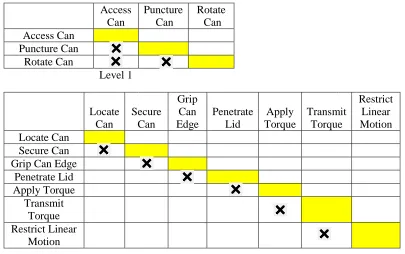
Step 4: Use DSM to verify if all the necessary relevant flows are available at a given
level of the functional decomposition and abstraction
Since there are many flows to keep track of, namely material, energy, information and parameters flows,
and since these flows are critical to compute the CDFs, it is necessary to ensure that all of the necessary
information is available at the appropriate level of abstraction or it that it can be derived from higher
levels of abstraction. In order to ensure this, a Design Structure Matrix (DSM) is developed for the system
under consideration. The DSM is a network modeling tool used to represent the elements of a system and
their interactions, thereby highlighting the system's architecture (or designed structure). The DSM has
many applications in the engineering of complex systems (Eppinger and Browning 2012.). In this step a
process-based DSM with sequential grouping is used to verify that all of the necessary material and
information flows have been identified at the appropriate level of decomposition by establishing a
horizontal relationship between each function. Implementation of this step will be discussed in detail in
section 4.2.
Step 5: Deploy the system stressor to each of the sub-functions in the function
hierarchy and establish a suitable measure for the equivalent life for each
sub-function to develop the corresponding CDF.
Once the DSM is completed, the next step is to develop a model to compute CDF. A comprehensive
review of different methods and models that could be used to compute remaining useful life and
ultimately CDF has been conducted and summarized in the literature review above. However, as
mentioned earlier, some of these methods are not applicable to the situation described in this work based
on the availability of data, time and costs of developing these models. Therefore, this section deals with
the computation of the CDF.
In order to compute the CDF it is necessary to develop a Failure Modes Effects and Criticality Analysis
30
compute the CDF. In order to represent the different methods that can be used to compute CDF, two
different methods will be given in the example in section 4.2. The first method involves using a reliability
model to compute remaining useful life and ultimately CDF. The second method is based on using the
available reliability data to develop a cumulative distributive function and use that data to compute a
CDF. It should be noted that these two classes of examples serve as a good guide for most of the specific
reliability models and approaches to estimate RUL that have been reviewed and are applicable to this
work.
4.2 Example
The application of this methodology to the manual can opener shown in figure 8 will be used to illustrate
more details of the approach. This can opener works by griping the edge of a can and is powered
manually to rotate the can which separates the lid from the can to allow access its internal contents. In the
remainder of this section, the 5-step methodology defined above will be applied to this product.
Figure 8: Can Opener
Step 1: Identify the main functional transformation of the system of interest and
identify the material, energy and information flows that are common to all systems
31
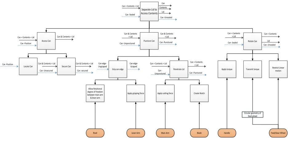
Figure 10 shows a functional decomposition of a can opener based on Esterman (2014) but it has been
modified to adhere to the principles outlined in section 4.1. The first step of a functional decomposition
(which is the focus of this first step in the CDF methodology) is to identify the primary function of the
system without considering the physical system that implements the functions and to identify the
associated flows (see Figure 9). Referring to figure 9, note that the general structure to represent a
function takes the form of a transformation taking place on the input flows to produce the output flows.
This also helps to identify the material and information flows associated with each function that should be
accounted for by all systems of the class. To reiterate, this will not include all flows that could be
transformed, only the ones that need to be transformed by all systems in this class. This same idea is
applied below as the functions are decomposed.
Can
Lid
Separate Lid to Access Contents
Can + Contents + Lid
Can -Sealed
Can -Unsealed Contents
32
Locate Can Can -Position
Allow Rotational degree of freedom between main arm & lever arm
Apply gripping force Apply cutting force Create Notch Puncture Can
Can & Contents + Lid
Can & Contents + Lid
Can -Unpunctured Can -Punctured
Apply torque Transmit torque
Rivet Lever Arm Main Arm Blade
Restrict Linear motion
Handle Feed/Gear Wheel
Circular geometry of feed wheel
Circular geometry of feed wheel Rotate Can Can + Contents
+ Lid
Can -Sealed
Can + Contents
Lid Can -Unsealed
Secure Can
Can & Contents + Lid Can & Contents + Lid
Can
Lid
Separate Lid to Access Contents
Can + Contents + Lid
Can -Sealed
Can -Unsealed Contents
Can -Unsecured Can -secured Access Can
Can + Contents + Lid Can & Contents + Lid
Can -Position
Penetrate Lid Can
-Unpunctured Can -Punctured Can + Contents + Lid Can + Contents + Lid Grip can edge
Can edge- Ungripped
[image:40.612.67.535.101.332.2]Can edge- Gripped
Figure 10: Functional decomposition of Can opener
Step 2: Develop the function hierarchy and identify the sub-functions of the
hierarchy
In this section, guidelines to decompose the top-level function will be given based on Gadre's (2016)
work. Functional decomposition should follow a tops-down approach i.e. functional decomposition
should start with the most primary or basic function of the system (which was defined in step 1). This
approach helps to maintain a degree of solution independence as the functions are decomposed. Consider
the functional decomposition of the can opener where it can be easily observed that there is no
assumption about the form of the solution for the top-level. However, by the second level of
decomposition, the architectural decisions to ‘puncture the can’ and ‘rotate the can’ have not been made.
The system could have rotated the tool or even used a chemical means to separate the lid. But note that
there are still many solution alternatives to ‘puncture the can’ or ‘rotate the can’. For example, the
puncture function can be accomplished with a piercing point or with a knife. This controlled convergence
in the reduction of the abstraction and the increase in solution detail is very useful for developing the
33
As one decomposes the function structure, at some point the structure reaches a point where the functions
are very low-level and the logical progression is that low-level function is implemented by a low-level
component (e.g. transmit torque might be implemented by a shaft). At the point it becomes necessary to
establish a relationship between the functions and the physical architecture of the system, switching to a
bottoms-up approach from the physical components to the functions is useful. Thus, a hybrid approach
which is a combination of both a tops-down and bottoms-up approach is found to be the most effective to
identify functions and reconcile the function structure.
One of the key challenges that was encountered in implementing this hybrid approach was the scenario
where a component mapped into more than one function, which will lead to issues in allocating
environmental impacts while developing the LCA. In order to overcome this scenario where the
component has a one-to-many relationship with the functions, the use of component features was
implemented. It is assumed that every component has a basic function and that there are features within
the component allow the components to perform additional functions. It was further observed that the
process steps that generated these features were easily accounted for and could be used as the basis for
allocating the environmental impacts. This is essentially an activity based approach toward the allocation
of the impacts.
Step 3: Identify user parameters and primary operational stressors:
User parameters define the usage patterns of the system and they are dictated by decisions made by the
user of the system. It is necessary to define user parameters because they scale the reference flows that
have been identified through the primary operational stressor and can be an independent parameter in the
CDF. Some guidelines to identify user parameters are summarized below:
1. For the main function, consider the reference flows and determine how they are affected by factors that
can be manipulated by the user. In this case that would be the number of cans and the types of cans being
34
2. For the sub-functions determine how its reference flows are impacted by the user parameters that were
identified for the function that the sub-functions integrate into. For example, consider ‘Puncture Can’, the
factors that users can manipulate that will impact this function include the type of can, the thickness of
can and the circumference of the can. This information can be derived from the user parameters of the
function that ‘Puncture Can’ integrates into, which are the number of cans and the type of can. These
user parameters can be used to model the CDF of the function based on the operational stressor. In the can
opener case example:
i. Usually cans are made of Aluminum
ii. The Aluminum thickness is 0.1 mm
iii. A typical can diameter is 66 mm
3. It may happen that some sub-functions may not have unique parameters which could be manipulated by
the users or some sub-functions may have an overlapping set of user parameters. For example, consider
‘Grip Can Edge’ and ‘Penetrate Can’ functions, both the functions have thickness as a common user
parameter
4.
As the tops-down and bottoms-up approaches to identify functions in the functional decomposition areapplied, further insights will also be generated that help to identify the user parameters.
The next step is to identify the operational stressor or stressors if it is a multifunction system. These
stressors are the external loads that act on each subsystem. The primary operational stressor is nothing
more than a user parameter which stresses the system. The primary operational stressor can be identified
from the primary function of the system and ultimately the primary operational stressor would also be
used as a parameter in the CDF equation in order to compute the remaining useful life. For example, in
the case of can opener the primary function is ‘Open Can’ thus the can is