Increasing eigenstructure assignment design degree of freedom using lifting

http://eprints.whiterose.ac.uk/117411/

Version: Published Version

Article:

Chen, Lejun, Pomfret, Andrew James orcid.org/0000-0003-0325-1617 and Clarke, Timothy

orcid.org/0000-0002-5238-4769 (2016) Increasing eigenstructure assignment design

degree of freedom using lifting. International Journal of Control. pp. 1-13. ISSN 0020-7179

https://doi.org/10.1080/00207179.2016.1236294

Reuse

Items deposited in White Rose Research Online are protected by copyright, with all rights reserved unless indicated otherwise. They may be downloaded and/or printed for private study, or other acts as permitted by national copyright laws. The publisher or other rights holders may allow further reproduction and re-use of the full text version. This is indicated by the licence information on the White Rose Research Online record for the item.

Takedown

If you consider content in White Rose Research Online to be in breach of UK law, please notify us by

For Peer Review

! "

For Peer Review

Vol. 00, No. 00, Month 20XX, 1–20

Increasing Eigenstructure Assignment Design Degree of Freedom using Lifting

(Received 00 Month 20XX; accepted 00 Month 20XX)

This paper presents the exposition of an output-lifting eigenstructure assignment (EA) design framework, wherein the available EA design degrees of freedom (DoF) is significantly increased, and the desired eigenstructure of a single-rate full state feedback solution can be achieved within an output feedback system. A structural mapping is introduced to release the output-lifting causality constraint. Additionally, the available design DoF can be further enlarged via involving the input-lifting into the output-lifting EA framework. The newly induced design DoF can be utilised to calculate a structurally-constrained, causal gain matrix which will maintain the same assignment capability. In this paper, the robustification of the output-lifting EA is also proposed, which allows a trade-off between performance and robustness in the presence of structured model uncertainties to be established. A lateral flight control benchmark in the EA literature and a numerical example are used to demonstrate the effectiveness of the design framework.

Keywords:lifting; eigenstructure assignment; causality constraint

1. Introduction

Eigenstructure assignment (EA) is a mature technique for the design of control systems, especially for flight control system (Alireza & Batool, 2012; B. Chen & Nagarajaiah, 2007; Clake, Ensor, & Griffin, 2003; Farineau, 1989; Kshatriya, Annakkage, Hughes, & Gole, 2007; G. P. Liu & Patton, 1998; Y. Liu, Tan, Wang, & Wang, 2013; Moore, 1976; Ouyang, Richiedei, Trevisani, & Zanardo, 2012; Piou & Sobel, 1994, 1995; Pomfret & Clarke, 2009; Shi & Patton, 2012; Wahrburg & Adamy, 2013; White, 1995; White, Bruyere, & Tsourdos, 2007). EA facilitates control system design by synthesizing a feedback gain matrix that exactly places the closed loop eigenvalues whilst matching the closed loop eigenvectors as closely as possible to a desired set. Some useful properties EA imbues on a system are: stability of response, appropriateness of transient response, decoupling of state or output response and disturbance rejection. Compared with many other competitive approaches exist to manipulate the eigenvalues of the closed-loop system and do not takes into account the role of the eigenvector, EA clearly exploits how system inputs affect mode dynamics and how these mode dynamics will be assigned to system states. Through defining a set of ideal closed-loop eigenstructure (e.g. eigenstructure which represents the realistic handling qualities of the flight control system), the realistic control effect will be guaranteed. In addition, the algorithm itself and the expression of the available design DoF can be highly visible. However, due to the lack of design DoF, e.g. the Kimura condition is not satisfied (Kimura, 1975), output feedback EA usually cannot fully assign the desired eigenstructure. This is an open problem which has been widely discussed in the literature (Andry, Shapiro, & Chung, 1983; L. Chen & Clarke, 2009; Clarke & Griffin, 2004; Pomfret, Clarke, & Ensor, 2005; Roppenecker & O’Reilly, 1989; Srinathkumar, 1978; Zhao & Lam, 2016a, 2016b).

Multirate control systems are those samplers and hold mechanisms that operate at more than one rate. Analysis and design methods for multirate control can be divided into two perspectives, the inferential control approach and the lifting approach (Tangirala, Li, Patwardhan, Shah, & Chen, 2

For Peer Review

2001) which is the focus of this paper. Lifting rearranges various input or output signals, working at different rates of a multirate system, using a uniform, slower frame rate, effectively increasing the number of system inputs and outputs.

This work introduces a formulation for output-lifted EA and first provides the solutions to deal with output-lifting causality constraints that naturally arise. The primary motivation for lifting is to significantly increase the available EA design DoF such that the desired eigenstructure only achievable through single-rate full state feedback solution can be achieved using an output feedback system. The combination of the output-lifting framework and EA effectively solve the open problem in EA literature wherein deign DoF is not enough for assigning eigenstructure.

By invoking the Gronwall Lemma, design DoF afforded by output-lifting framework are utilized to derive a time-domain stability robustness measure of output-lifted system in the presence of uncertainty. The Gronwall Lemma was adopted in B. S. Chen and Wong (1987) and Sobel, Banda, and Yeh (1989b) to deduce a time domain robustness measures taking into account of structured and unstructured uncertainties, respectively. The results were extended to discrete system in Sobel, Banda, and Yeh (1989a) and the conservatism of the measure was reduced through using Perron weighting. This paper extends the results from Sobel et al. (1989a); Yu, Piou, and Sobel (1993) and allows the location and the sensitivity of individual eigenvalues can be operated on rather than the spectrum of the all of the system eigenvalues. This further improves the design conservatism. Due to extra DOF offered by output-lifting, a multi-objective optimisation is deduced by taking into account of the trade-off between system stability robustness and mitigation of degradation in equivalent full state feedback performance.

Output-lifting will necessitate a causality constraint which requires structural changes to the gain matrix, a structure mapping is proposed, wherein a directly-calculated, non-causal gain matrix can be utilized to generate a new closed-loop system structure that alleviates the causality constraint. In addition, the available design DoF can be further enlarged by adding input-lifting to the output-lifting EA framework. The newly introduced design DoF can be utilised to calculate a structurally-constrained, causal gain matrix which will maintain the same assignment capability.

The paper is organized as follows. In Sections 2, EA and lifting are briefly introduced. Section 3 proposes output-lifting EA. A less conservative time-domain robustness measurement is developed in Section 4 to ensure the robustification of output-lifting EA. In Section 5, a structure mapping is introduced to alleviate the causality constraint induced by output-lifting. The proposed approaches are demonstrated using a well-known example taken from EA literature and the simulation results are shown in Section 6. By using extra DoF that input-lifting can benefit, a structurally-constrained, causal, lifted controller can be found directly in Section 7 and the associated numerical example is given in Section 8. Concluding remarks are given in Section 9.

2. Preliminary

Consider a continuous-time, controllable and observable linear time-invariant system, given by

˙

x=Acx+Bcu

y=Ccx

(1)

whereAc ∈Rn×n, Bc ∈Rn×r, Cc ∈Rm×n and Dc ∈Rm×r.

Consider a multirate control system, wherein the hold circuit and the sampler work with sample

periods ofqiTb and poTb respectively. Tb is the base sampling period of the system, which can be

any common factor of the input and output sampling periods. The main sampling period of the

system is given byT =l.c.m(po, qi)∗Tb,l.c.mstands for least common multiple. According to the

framework for lifting summarized in T. Chen and Francis (1995), the system inputs and outputs 2

For Peer Review

are lifted byq and p, respectively, where

q= l.c.m(po, qi) qi

p= l.c.m(po, qi) pi

(2)

The resulting state space lifted system is expressed as

x(k+ 1) =ALx(k) +BLu¯(k)

¯

y(k) =CLx(k) +DLu¯(k)

(3)

wherex(k) :=x(kT), and the lifted inputs and outputs are given by

¯ u(k) =

      

u(kT) u(kT+pTb)

u(kT+ 2pTb)

.. .

u(kT + (pq−p)Tb)

       ¯ y(k) =

      

y(kT) y(kT+qTb)

y(kT + 2qTb)

.. .

y(kT + (pq−q)Tb)

      

In (3), matrices AL∈Rn×n, BL∈Rn×qr, CL ∈Rpm×n and DL∈Rpm×qr are

AL BL

CL DL

=           

Apq pqP−1 i=pq−p

Ai_B pq−Pp−1 i=pq−2p

Ai_{B · · ·} pP−1 i=0

Ai_B

C D₀,0 D0,1 · · · D0,q−1

CAq D1,0 D1,1 · · · D1,q−1

CA2q D2,0 D2,1 · · · D2,q−1

..

. ... ... . .. ...

CApq−q Dp−1,0 Dp−1,1 · · · Dp−1,q−1

          

where A, B, C and D are deduced via a discretization of system (1) and the element D(i, j) is

given by

Di,j = DX[jp,(j+1)p)(iq) +

(j+1)p−1

X

h=jp

CAin−1−hBX[0,iq)(h) (4)

where the characteristic function on integers, X[a,b)(h), conditionally nulls elements within the

matrixDL,

X[a,b)(h) =

I a≤h < b

0 otherwise

Obviously, lifting will enlarge the number of system inputs and outputs (r →qr andm →pm):

the design DoF is enlarged. The extra free elements can be parameterised to more closely achieve specified design requirements.

3. Output-lifted Eigenstructure Assignment

For Peer Review

tem of (3), wherein DL is non-null (pathological conditions of choosing base sampling frequency

and desired eigenvalues to prevent controllability and observability of (3) are described in T. Chen and Francis (1995) and Sheng, Chen, and Shah (2002)).

Assume the system outputs are lifted by a factor p and the matrix CL satisfies row(CL) =

pm ≥ rank(CL) = n, where row(CL) represents the number of rows of CL, a static control law

¯

u(k) =Ky¯(k) + ¯r(k) is applied to the lifted system to yield

x(k+ 1) = (AL+BLN CL)x(k) + (BL+BLN DL)¯r(k)

¯

y(k) = (CL+DLN CL)x(k) + (DL+DLN DL)¯r(k)

where ¯r is the lifted exogenous input and

N = (I −KDL)−1K (5)

Remark 3.1: In (5), this time, the term I−KDL in N is assumed to be nonsingular. The

con-straint is not a curiosity of the exposition presented here. Rather, it represents a system singularity. The feedforward matrix and the feedback matrix form direct forward and backward transmission paths, coupling the input and output through a pair of simultaneous equations. When the constraint is not satisfied, no instantaneous solution exists to these equations for y¯ given r¯and x. Thus the constraint is somewhat pathological; it is reasonable to assume that a control system design ap-proach based on meeting performance goals would never give rise to such a situation. Nevertheless, ensuring that this is the case is a simple matter in most cases. This issue will be discussed later in the analysis of the algorithm.

Using the fact that the distinct eigenvalue/eigenvector pair of the closed-loop lifted system,λi

andvi, satisfy

(AL+BLN CL)vi = λivi (6)

0 = [AL−λiI BL]

vi

N CLvi

(7)

vi

N CLvi

thus belongs to the nullspace of [AL−λiI BL].

For somefi ∈Cqr×1,

vi

N CLvi

=

Pi

Qi

fi (8)

where

range

Pi

Qi

=null([AL−λiI BL]) (9)

and Pi ∈ Cn×qr is an orthonormal basis for the allowable subspace used to select vi. Once the

design vector,fi has been established, the matrices V, S can be calculated through

V = [v1. . . vl] = [P1f1. . . Plfl] (10)

S=N CLV = [Q1f1. . . Qlfl] (11)

For Peer Review

Substituting (5) into (11) to obtain

S = (I −KDL)−1KCLV =K(DLS−CLV) (12)

The gain matrix may be recovered by finding

K = S(CLV +DLS)†

+Z(I−(CLV +DLS))(I−(CLV +DLS)†) (13)

where, (·)† _{is the Moore-Penrose inverse operation andZ is the free matrix to be parameterised. l}

represents thelth assigned eigenvector and associated eigenvalue. Clearly, (13) holds only ifl≤pm.

Consequently for an original un-lifted output feedback system (p=1), a maximum of m poles can

be assigned and the other (n−m) remain unassigned and may become unstable due to the lack

of design DOF to parameterise the allowed right eigenvector subspace. For output lifting system,

supposepm≥n, (13) holds and the desired eigenstructure of full state feedback can be assigned.

Following the discussion in Remark 3.1, Theorem 3.1 is proposed here to avoid the pathological

condition that the termI−KDL becomes singular.

Theorem 3.1: By suitably choosing the set of desired eigenvectors, such thatI−DLS(CLV+DLS)

is singular, Z can be parameterized to ensure the non-singularity of I−KDL.

Proof: Supposex∈ker(CLV +DLS) andQ=S(CLV +DLS)†+Z, it is easy to choose a free

parameterZ, such thatI−DLQis nonsingular - i.e. there must not exist a zero-valued eigenvalue

forI−DLQ. That is, DLQmust have no eigenvalues of unit value. So

DLQx6=x (14)

DL(S(CLV +DLS)†+Z)x6=x (15)

For anyx∈ker(CLV +DLS),

Zx=Z(I−(CLV +DLS)(CLV +DLS)†)x (16)

then (15) can be written as

(I −DLS(CLV +DLS)†

−DLZ(I−(CLV +DLS)(CLV +DLS)†))x6= 0 (17)

Using the expression ofK in (13), (17) can be written as

(I −DLK)x6= 0 (18)

Supposey∈range(CLV +DLS), it follows

Z(I−(CLV +DLS)(CLV +DLS)†)y= 0 (19)

By suitably choosing a set of desired eigenvectors, such thatI−DLS(CLV +DLS) is nonsingular:

(I −DLS(CLV +DLS))y6= 0 (20)

For Peer Review

Substituting (19) to (20) to yield

(I−DLS(CLV +DLS)†

−DLZ(I −(CLV +DLS)(CLV +DLS)†))y6= 0

(21)

that is (I−DLK)y6= 0.

The range and kernel describe a complete space,

Rn_{=range(CLV +DLS)⊕ker(CLV +DLS) (22)}

For any vectorz in full space, where{z}={x} ∪ {y}

(I−DLK)z6= 0 (23)

Since the non-singularity of I−DLK is necessary and sufficient to ensure the non-singularity of

I−KDL (Fletcher, 1981),Z can be chosen to ensure the termI−KDL to be nonsingular.

The gain matrix can be recovered sincerank(CL) =n≤row(CL). Using thisK, the equivalent

of state feedback EA can be achieved since the allowable subspaces of output-lifting feedback and state feedback corresponding to each desired eigenvalue are same, the proof of which is in Theorem 3.2 below.

Theorem 3.2: Suppose As, Bs is a discrete-time system working at the main sampling period,

the allowable subspace of the output-lifted system is the same as for the single main sampling rate system.

null([AL−λiI, BL]) =null([As−λiI, Bs]) (24)

Proof: Let Ac, Bc, Cc, Dc and A, B, C, D represent a continuous-time system and an equivalent

system sampled at a base sampling period,Tb.A and B can be given by

A=eTbAc _B

=

Z Tb

0

eτ Ac_{dτ B}

c (25)

Suppose system outputs are lifted by a ratiop, the main sampling period becomespTb, and

As = epTbAc =Ap (26)

Bs =

Z pTb

0

eτ Ac

dτ Bc = p

X

i=1

Z iTb

(i−1)Tb

eτ Ac

dτ Bc (27)

Using the integral identity

Z β

α

f(x)dx= β−α

ψ−ϕ

Z ψ

ϕ

f(β−α

ψ−ϕτ+

βψ−αϕ

ψ−ϕ )dτ (28)

For Peer Review

Equation (27) can be written as

Bs =

p

X

i=1

Z iTb

(i−1)Tb

eτ Ac_{dτ B}

c

=

Z Tb

0

eτ Ac

dτ Bc+ p

X

i=2

Z iTb

(i−1)Tb

eτ Ac

dτ Bc (29)

=

Z Tb

0

eτ Ac

dτ Bc+ p−1

X

i=1

Z iTb

(i−1)Tb

e(τ+iTb)Ac

dτ Bc (30)

=

Z Tb

0

eτ Ac

dτ Bc+ p−1

X

i=1

eiTbAc Z Tb

0

eτ Ac

dτ Bc (31)

=

p−1

X

i=0

(Ai)B =BL (32)

Therefore, by inspection, (24) is true.

4. Robustification

In this section, the design DoF generated by output-lifting framework is utilized in a post assign-ment process, to achieve the robustification of the output-lifting EA. A multi-objective optimisation is established to improve the stability robustness, whilst to mitigate the degradation in equivalent full state feedback performance.

4.1 Robustness measure with time-varying uncertainty

Suppose the lifted system is subject to time-varying parametric structured uncertainty

∆AL(k),∆BL(k),∆CL(k) and ∆DL(k), satisfy ∆AL+(k) ≤ Am, ∆BL+(k) ≤ Bm, ∆CL+(k) ≤ Cm,

and ∆D_L+(k)≤Dm. In this paper, (·)+ replaces the entries of matrix by their absolute values and

(·)m represents the absolute value of the maximum variation of time varying uncertainties, on an

element by element basis. A stability robustness measure for an output-lifted system is defined in Theorem 4.1.

Theorem 4.1: The uncertain closed-loop system is asymptotically stable for all∆AL(k),∆BL(k),

∆CL(k) and ∆DL(k) if

n

X

i=1

(wi)+(Acm+EmΞ)(vi)+

1− |λi|

<1 (33)

where

Acm = Am+Bm(N CL)++ (BLN)+Cm+BmN+Cm

Em = (BLN)+Dm+BmN+Cm (34)

Ξ = (I−N+Dm)−1(N+(CL++Cm) (35)

andV and λi are the modal matrix and theith eigenvalues of (AL+BLN CL) respectively. wi and

vi are achieved left and right eigenvectors associated withλi. 2

For Peer Review

Proof: See Appendix A.

Remark 4.1: Note that minimization of the left side of (33) will increase the stability robustness of the system. A large denominator in (33) indicates that the eigenvalue is far away from the unit circle, which exhibits greater stability robustness. Also, choosing different eigenvectors directions to decrease the numerator of (33) can be considered as reducing the sensitivity of the closed-loop system to the given structured perturbation.

From the left side of (33), the stability robustness of the itheigenvalue/eigenvector pair can be

measured by using (36).

Jsi= min

fi,λi

(wi)+(Acm+EmΞ)(vi)+

1− |λi|

(36)

4.2 Multi-objective output-lifting EA

Criteria associated with retaining full state feedback performance is also considered alongside robustification. In this paper, the performance measure is proposed to minimise the errors between the desired and the achieved eigenstructure. A cost function as shown in (37) is used to fulfil the task.

Jvi = min

fi,λi

kvid−Pifik2₂ (37)

s.t.|λid−λia|< r

wherefi andvid represent theith design vector and theith desired right eigenvector.k · kdenotes

the vector or matrix 2-norm.λidandλiarepresent the desired and achieved eigenvalue, respectively.

Pi is the allowable subspace for the ith achieved eigenvalue. r is the radius of the allowed region

for theith eigenvalue.

In improving the stability robustness, whilst, mitigating the performance degradation, a multi-objective optimisation is given by

Ji =aiJsi+biJvi (38)

where,Jsi, defined in (36), represents the stability robustness measure. The weighting parameters

ai and bi control the relative significance of the robustness and the performance terms of the ith

eigenvalue/eigenvector pair.

5. Releasing causality constraints using structure mapping

Since the outputs of the controller at current time only depend on the output of the plant at or before current time, lifting system outputs will introduces causality constraints upon the constant gain matrix. For example, suppose lifting system inputs and outputs as defined in (4), the resulting

feedback gain matrix K must be lower triangular, under causality. With the causality constraint

enforced, anyfully-populated gain matrix, calculated as a general outcome of the direct use of EA

on an output-lifted system is non-causal and even unstable.

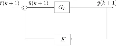
In this section, a structure mapping is proposed to release the causality constraint, whilst allowing the non-causal full gain matrix to be utilised. The structure mapping is achieved through the change of implementation structure of the closed-loop system, which is shown in Figs. 1 and 2.

For Peer Review

+ +

¯

r(k+ 1) u¯(k+ 1)

GL

K

¯ y(k+ 1)

Figure 1. Closed-loop structure under causality constraint

+ + +

¯ u(k+ 1)

Z−1 GL

H

L

M ¯

r(k+ 1) u¯(k) y¯(k)

Figure 2. Closed-loop structure without causality constraint

In Fig. 1, the direct-calculated non-causal gain matrixK satisfies

¯

u(k+ 1) = Ky¯(k+ 1) + ¯r(k+ 1) (39)

= K[CLx¯(k+ 1) +DLu¯(k+ 1)] + ¯r(k+ 1)

= NCL(ALx¯(k)+BLu¯(k))+(I−KDL)−1r¯(k+1)

where the termI−KDis assumed to be nonsingular (the implications of this restriction is discussed

earlier). In Fig. 2, the new implementation structure releases the causality constraint. Appropriate equations can be obtained directly from the figure.

¯

u(k+ 1) = Lu¯(k) +My¯(k) +Hr¯(k+ 1) (40)

= Lu¯(k) +M DLu¯(k) +M CLx¯(k) +H¯r(k+ 1)

A mapping between (39) and (40) are given by

M CL = N CLAL (41)

L+M DL = N CLBL (42)

H = (I−KDL)−1 (43)

Using above structural mapping, matrices M, L and H can be calculated based on non-casual

matrixK. The causality constraint is released and the eigenstructure of the closed-loop system in

Fig. 1 can be maintained. 2

For Peer Review

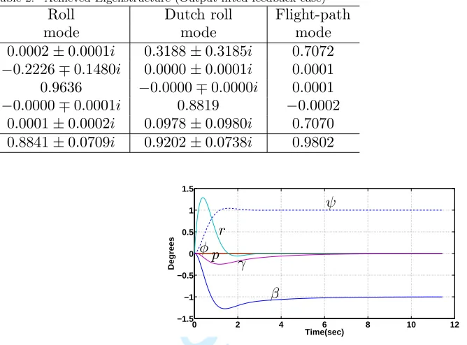
Table 1. Achieved Eigenstructure (Full state feedback case)

Roll Dutch roll Flight-path

mode mode mode

0.0002±0.0001i 0.3188±0.3185i 0.7072

−0.2226∓0.1480i 0.0000±0.0001i 0.0001

0.9636 −0.0000∓0.0000i 0.0001

−0.0000∓0.0001i 0.8819 −0.0002

0.0001±0.0002i 0.0978±0.0980i 0.7070

0.8841±0.0709i 0.9202±0.0738i 0.9802

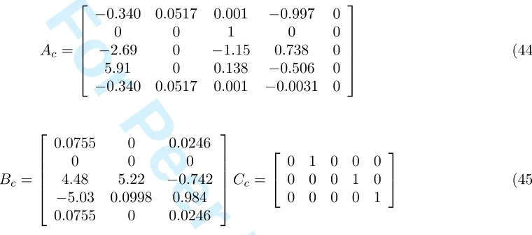
6. Example 1

A fifth-order FPCC Lateral Dynamics Flight Control benchmark within the EA literature (Sobel & Lallman, 1989) is illustrated here. The continuous-time state space system is given by

Ac =

     

−0.340 0.0517 0.001 −0.997 0

0 0 1 0 0

−2.69 0 −1.15 0.738 0

5.91 0 0.138 −0.506 0

−0.340 0.0517 0.001 −0.0031 0

     

(44)

Bc =

     

0.0755 0 0.0246

0 0 0

4.48 5.22 −0.742

−5.03 0.0998 0.984

0.0755 0 0.0246

     

Cc =





0 1 0 0 0 0 0 0 1 0 0 0 0 0 1



 (45)

The states [β φ p r γ]′ _{correspond to sideslip angle, bank angle, roll rate, yaw rate and flight}

path angle, respectively. The control inputs [δr δaδc]′ denote the surface deflections of the rudder,

ailerons and vertical canard respectively. The desired eigenvalues, corresponding to Dutch roll,

Roll and Flight path modes are λd_dr = −2±j2, λd_roll = −3±j2 and λd_s = −0.5, respectively.

The design goal is a yaw pointing/lateral translation control law in which the lateral/directional flight-path response is decoupled from the yaw rate response. Also, both of these responses should be decoupled from the roll rate and bank angle response. Hence, the desired eigenvectors are chosen as:

v_drd =0 0 0 1 0T ±j1 0 0 1 0T

vd_roll=0 0 1 0 0T ±j0 1 1 0 0T

vd_s =1 0 0 0 1T

(46)

Suppose the holder and the sampler works at the main sampling period 0.04sec and the base

sampling period 0.01sec, respectively. The system outputs are chosen to be lifted by 4. After

discretisation at the main sampling period, the desired eigenvalues for the roll, Dutch roll and

flight-path modes become 0.8804±0.0709i, 0.9202±0.0738i, 0.9802 in the unit circle.

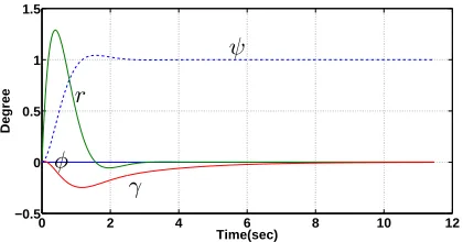
Full state feedback EA and output-lifted EA are both implemented on benchmark. Results are presented to demonstrate the equivalence of performance. In tables 1 and 2, top and bottom rows show the achieved eigenvectors and eigenvalues, respectively. Clearly, output-lifting EA can achieve the same eigenstructure as achieved using full state feedback. Figs. 5 and 6 show the nominal 2

For Peer Review

Table 2. Achieved Eigenstructure (Output-lifted feedback case)

Roll Dutch roll Flight-path

mode mode mode

0.0002±0.0001i 0.3188±0.3185i 0.7072

−0.2226∓0.1480i 0.0000±0.0001i 0.0001

0.9636 −0.0000∓0.0000i 0.0001

−0.0000∓0.0001i 0.8819 −0.0002

0.0001±0.0002i 0.0978±0.0980i 0.7070

0.8841±0.0709i 0.9202±0.0738i 0.9802

0 2 4 6 8 10 12

−1.5 −1 −0.5 0 0.5 1 1.5

Time(sec)

Degrees

ψ

r φ

γ p

β

Figure 3. Full State Feedback Responses to a Unit Heading Command

0 2 4 6 8 10 12

−0.2 0 0.2 0.4 0.6 0.8 1 1.2

Time(sec)

Degree

r φ

γ

ψ β

p

Figure 4. Full State Feedback Responses to a Flight-Path Command

outputs responses of output-lifted system to unit heading and flight-path commands respectively, wherein, the nominal mode decoupling information is shown, which is same as that of a full state feedback design as shown in Figs. 3 and 4, representing the best possible performance.

Continuous-time structured uncertainty is assumed, in line with the literature, to be of the form

∆Ac =

     

0.1 0 0 0 0

0 0 0 0 0

0 0.1 0 0 0

0 0 0.1 0 0

0 0 0 0.1 0

     

,∆Bc = 0 (47)

The allowed migration regions for the real and imaginary parts of the eigenvalues of the dutch

roll, roll and flight-path modes are 0.03, 0.03, and 0.01 respectively.

The solution of nominal output-lifted system offers relatively poor robustness since the value of

left hand side of (33) equates to 1.4769. In view of increasing the stability robustness of the system,

two robust solutions of the gain matrices are given. In calculating one solution, increasing stability 2

For Peer Review

0 2 4 6 8 10 12

−0.5 0 0.5 1 1.5

Time(sec)

Degree

ψ

r

φ γ

Figure 5. Lifted Output Responses to a Unit Heading Command

0 2 4 6 8 10 12

−0.2 0 0.2 0.4 0.6 0.8 1 1.2

Time(sec)

Degree

r φ

γ

Figure 6. Lifted Output Responses to a Flight-Path Command

0 5 10 15 20

−0.4 −0.2 0 0.2 0.4 0.6 0.8 1 1.2

Time(sec)

Degree

r

φ γ

Figure 7. Lifted Output Responses to a Unit Heading Command after robustification without performance protection

robustness without performance protection is considered, that is, in (38), ai = 10, bi = 0 (i =

1, . . . , n). This solution yields a value of 0.3845 for the left hand side of (38), which demonstrates better robustness.

Another solution is calculated, combing the performance protection. In this case,ai, bi = 1 (i=

1, . . . , n) in (38), a value of 0.9487 is yielded for the left hand side of (33). Compared with the value calculated under the circumstances not involving performance protection, the robustness is reduced and the performance is improved.

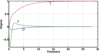
The following time histories demonstrate the results of the robustification.

Fig. 7 and Fig. 8 depict output responses to unit heading and flight-path commands without performance protection. Output responses to unit heading and flight-path commands with perfor-mance protection is shown in Figs. 9 and 10. These figures show that perforperfor-mance protection has done a lot to preserve the decoupling action of the controller although, as expected, responses have suffered some degradation due to robustification.

For Peer Review

0 5 10 15 20 25 30

−0.5 0 0.5 1

Time(sec)

Degree

r

φ

γ

Figure 8. Lifted Output Responses to a Flight-Path Command after robustification without performance protection

0 2 4 6 8 10 12 14

−0.5 0 0.5 1 1.5

Time(sec)

Degree

r

φ γ

Figure 9. Lifted Output Responses to a Unit Heading Command after robustification with performance protection

0 2 4 6 8 10 12 14

−0.2 0 0.2 0.4 0.6 0.8

Time(sec)

Degree

r φ

γ

Figure 10. Lifted Output Responses to a Flight-Path Command after robustification with performance protection

7. Input-lifting benefits

Lifting system inputs can increase the dimension of the allowable subspace P_iT QT_i T

so that each desired eigenvector can be exactly achieved (i.e. all of the elements in each) (Patton,

Liu, & Patel, 1995). Lifting system outputs can be used to enable assignment of all of the desired

eigenvectors. Therefore, if system inputs and outputs arebothlifted (dual-lifting), all of the desired

eigenvectors can be exactly achieved. As an additional bonus, since the size of the gain matrix is increased considerably after the dual-lifting process, many elements in the gain matrix are still available, as further design freedom, and can be parameterised.

As mentioned in the last section, lifting system outputs induces a causality constraint such that, either a structural mapping must be invoked, or some elements in the gain matrix must be nulled, resulting in a directly-causal gain matrix of appropriate form. It is possible to parameterise and 2

For Peer Review

exploit some of the extra DoF, described above, to impose this structure. So, if the available DoF

are larger or equal to the sum of the DoF used for assigning eigenstructure and satisfying the

causality constraint, then a solution for the EA gain matrix which simultaneously satisfies the causality constraint can be found directly. The procedure for this is now presented.

Proposition 7.1: For the dual-lifting case, wherein subsets of samplers or hold circuits works at different rates, the distribution of the DoF for finding a directly-causal gain matrix is given by

r

X

i=1

qin+t≤ r

X

i=1

m

X

j=1

qipj (48)

t=

r

X

i=1

m

X

j=1

qipj−(rm+ r

X

i=1

qi−1 X

k=1

m

X

j=1

round(kpj qi

+1)

) (49)

wheretequates the number of the fixed null elements inside the gain matrix constrained by causality. qi and pi are lifting ratios of the ith input and output respectively.

After choosing suitable dual-lifting ratios to satisfy Proposition 1, the free parameter matrix Z

in (13) can be used to formulate a causal gain matrix. This process for finding a suitableZ matrix

can be achieved by using a permutation matrixUδ×mprq (Pomfret, 2006), δ is the number of the

null elements of the gain matrix caused by the causality constraint. In each row of U, only one

element is unity, others are all null, which can be used to select the specified elements of the vector

version of the gain matrix. Therefore, all null elements in the gain matrix are selected by usingU,

which is given by

U vec(K) = 0 (50)

wherevec(·) denotes column-wise vectorisation of a matrix. Substituting (13) into (50) yields

U vec(K) = 0 (51)

U vec(K0+Z(I−Y Y†)) = 0 (52)

U vec(K0) +U vec(Z(I−Y Y†)) = 0 (53)

whereK0 =S(CLV +DLS)†and Y =CLV +DLS.

Applying the identityvec(AY B) = (BT ⊗A)vec(Y) to (53) yields

U vec(K0) +U((I−Y Y†)T ⊗I)vec(Z) = 0 (54)

Define Ξ = (I −Y Y†)T _{⊗I, (54) can be written as}

UΞvec(Z) =−U vec(K0) (55)

Provided the identity UΞ is a full row rank, it follows

vec(Z) =−(UΞ)†U vec(K₀) + (I−(UΞ)†UΞ)vec(Ze) (56)

where Ze represents a free matrix. If rank(UΞ) = δ, and DoF of the lifted system satisfies (48),

the free matrix Z in (13) can be find and the causal matrix K can be calculated to assign the

eigenstructure under the causality constraint. 2

For Peer Review

To demonstrate direct-causal feedback gain matrix design, consider the following system and its desired eigenstructure (Patton et al., 1995):

A=





0 1 0

0 0 1

−6 −11 −6



B=

  1 1 0 1 1 1 

C =





1 0 0 0 1 0 0 0 1



 (57)

λ={−0.5,−0.6,−0.7} Vd=



 1 0 00 1 0

0 0 1



 (58)

Let the main sampling period be 0.1sec and the two holds operate at periods of 0.05sec and

0.02sec, respectively. Three samplers are assumed to work at periods of 0.02sec, 0.05secand 0.1sec,

respectively. The lifting ratios of two system inputs are selected to be 2 and 5, respectively, and those of three system outputs are selected to be 5, 2 and 1, respectively. The desired discrete eigenvalues are given by

λdis={0.9512,0.9418,0.9324} (59)

Notice that the causality constraint requires that the structure of the causal gain matrix to satisfy

         

u1(0s)

u₁(0.05s) u2(0s)

u2(0.02s)

u2(0.04s)

u2(0.06s)

u2(0.08s)

          =          

× 0 0 0 0 × 0 ×

× × × 0 0 × × ×

× 0 0 0 0 × 0 ×

× × 0 0 0 × 0 ×

× × × 0 0 × 0 ×

× × × × 0 × × ×

× × × × × × × ×           ·            

y₁(0s) y1(0.02s)

y1(0.04s)

y₁(0.06s) y1(0.08s)

y₂(0s) y2(0.05s)

y₃(0s)

           

where′_×′_{represent the free elements to be parameterized and the zero elements denote the causality}

constraints.

Recall (48), in this example,t= 20,Pr_i=1qin= 21,Pri=1

Pm

j=1qipj = 56. Since the distribution

of DoF satisfies (48), the matrixZ can be calculated using (56).

Z=          

1.61 1.83 −3.77 −4.11 1.06 −6.40 0.43 −2.64

0.16 −0.82 −1.57 3.96 −0.72 1.33 0.43 0.77

2.24 1.87 −4.59 −4.98 0.98 −7.89 −0.01 −3.48

0.23 2.54 −2.56 −2.77 0.49 −3.55 −0.10 −1.60

0.01 0.08 0.14 −0.32 −0.05 −0.09 −0.17 −0.11

0.19 0.15 0.13 0.12 −0.66 −0.03 −0.06 −0.04

0.00 0.00 0 0 0 0 0 0

For Peer Review

Substituting matrix Z into (13) to yield a directly-causal gain matrix Kc, given by

Kc=

         

−7.56 0 0 0 0 −13.41 0 −4.79

8.22 0.59 −5.22 0 0 7.07 0.24 4.37

−8.10 0 0 0 0 −15.44 0 −7.46

−5.37 1.58 0 0 0 −7.59 0 −4.04

−0.36 0.10 0.45 0 0 −0.25 0 −0.83

5.61 1.26 −2.05 −2.26 0 4.10 0.21 1.16

11.81 2.32 −4.92 −5.37 1.32 8.85 0.36 3.31

         

andU vec(Kc) = 0. UsingKc, the desired eigenstructure is achieved.

9. Conclusions

Through exposing design DoF induced by output-lifting EA, the desired eigenstructure of a single-rate full state feedback solution can be achieved with an output feedback system, and output-lifting causality constraint is released by the structural mapping. In addition, the available design DoF can be further enlarged via involving the input-lifting in the output-lifting EA framework. The newly introduced design DoF can be utilised to calculate a structurally-constrained, causal gain matrix which will maintain the same assignment capability. In addition, a less conservative time-domain robustness measurement is developed to ensure the robustification of output-lifting EA.

Appendix. A

Proof of Theorem 4.1

Consider an lifted system with time-varying uncertainty

x(k+ 1) = (AL+ ∆AL(k))x(k) + (BL+ ∆BL(k))¯u(k) (60)

¯

y(k) = (CL+ ∆CL(k))x(k) + (DL+ ∆DL(k))¯u(k) (61)

¯

u(k) = Ky¯(k) (62)

Substituting (61) into (62) yields

(I−KDL)¯u(k) = K(CL+ ∆CL(k))x(k) +K∆DL(k)¯u(k) (63)

From (63),

¯

u(k) =N(CL+ ∆CL(k))x(k) +N∆DL(k)¯u(k) (64)

Now substitute (64) into (60) to obtain

x(k+ 1) = Aclx(k) + ∆Acl(k)x(k) + ∆E(k)¯u(k) (65)

where

∆Acl(k) = ∆AL(k) + ∆BL(k)N CL+ (B+ ∆BL(k))N∆CL(k) (66)

Acl = AL+BLN CL (67)

∆E(k) = (BL+ ∆BL(k))N∆DL(k) (68)

LetM represent the modal matrix of AL+BLN CL and define matrix D as a diagonal matrix

with real positive entries, then M D also represents a modal matrix. Using the modal similarity

For Peer Review

transformation, it follows

x(k) =D−1M−1z¯(k) (69)

Applying the similarity transformation to (65) and the solution of ¯z(k) is given by

¯

z(k) = D−1ΛkDz¯(0) +

k+1

X

j=0

Λk−j−1D−1M−1∆Acl(j)M Dz¯(j)

+

k+1

X

j=0

Λk−j−1D−1M−1∆E(j)¯u(j) (70)

where Λ is a diagonal matrix of the eigenvalues ofAc. Applying the absolute value operator to get

¯

z+(k) ≤ D−1Λk_Dz¯+_{(0) +}

k+1

X

j=0

Λk−j−1_D−1_(M−1₎+_∆A

cl(j)M+Dz¯+(j)

+

k+1

X

j=0

Λk−j−1_D−1_(M−1₎+_∆E(j)¯u+_{(j) (71)}

Also, (64) can be written as

¯

u+(k) =N+(C_L++Cm)x+(k) +N+Dmu¯+(k) (72)

Then

¯

u+(k)≤ΞM+Dz¯+(k) (73)

Substituting (73) into (71) yields

¯

z+(k) ≤ D−1ΛkDz¯+(0) +

k+1

X

j=0

Λk−j−1D−1(M−1)+∆Acl(j)M+Dz¯+(j) (74)

+

k+1

X

j=0

Λk−j−1D−1(M−1)+∆E(j)ΞM+Dz¯+(j)

Using the fact thatkΛkk ≤αk and α=max|Λ|, it follows

¯

z+(k) ≤D−1akDz¯+(0) +

k+1

X

j=0

αk−j−1D−1(M−1)+(Acm+EmΞ)M+Dz¯+(j) (75)

Then

¯

z+(k)α−k ≤z¯+(0) +

k+1

X

j=0

α−1D−1(M−1)+(Acm+EmΞ)M+Dα−jz¯+(j) (76) 2

For Peer Review

Using the Discrete Gronwall Lemma, (76) can be written as

¯

z+(k)α−k ≤z¯+(0)(1 +α−1(D−1(M−1)+(Acm+EmΞ)M+D))k (77)

Now multiply both sides of (77) byαk _{and then take the norm for both sides of (77) to obtain}

kz¯+(k)k ≤ kz¯+(0)k(α+kD−1(M−1)+(Acm+EmΞ)M+Dk)k (78)

From (78), a sufficient condition for the asymptotically stable response is given by

kD−1(M−1)+(Acm+EmΞ)M+Dk<1−α (79)

which equates to

k(M−1)+(Acm+EmΞ)M+k2D <1−α (80)

Since the matrix term inside the norm of the above equation only contains the positive elements, the condition in (80) can be written as

inf

D k(M

−1₎+_(A

cm+EmΞ)M+k2D <1−α (81)

Using the fact that

inf

D kA

+_k

2D =ρ(A+) (82)

whereρrepresents the perron eigenvalue of the matrix with all positive entries. (81) can be written

as

ρ[(M−1)+(Acm+EmΞ)M+]<1−α (83)

Since the eigenvalues ofAB and ofBAare identical for all square Aand B, (83) equates to

ρ[M+(M−1)+(Acm+EmΞ)]<1−α (84)

Dividing both sides of (84) by (1−α) yields

ρ[M

+_(M−1₎+_(A

cm+EmΞ)

1−α ]<1 (85)

which equates to

ρ[

Pn

i=1v+i (wi)+(Acm+EmΞ)

1−α ]<1 (86)

Using this result, if A+≤B+, then

λmax(A+)≤λmax(B+) (87)

For Peer Review

Substitute (87) into (86) and invoke the property|Λk_{| ≤α}k_{, a sufficient condition is given by}

ρ[

n

X

i=1

v_i+(wi)+(Acm+EmΞ)

1− |λi|

]<1 (88)

The spectral radius of the square matrices A,B satisfies (89), which can be proven by using

Rayleigh’s principle.

ρ(A) +ρ(B)≥ρ(A+B) (89)

Applying the above matrix property to (88) to get

n

X

i=1

ρ[v

+

i (wi)+(Acm+EmΞ)

1− |λi|

]<1 (90)

which can be simplified by

n

X

i=1

(wi)+(Acm+EmΞ)v+i

1− |λi|

<1 (91)

References

Alireza, E. A., & Batool, L. (2012). Application of matrix perturbation theory in robust control of large-scale systems. Automatica, 48(8), 1868–1873.

Andry, A. N., Shapiro, E. Y., & Chung, J. C. (1983). Eigenstructure assignment for linear systems. IEEE Transactions on Aerospace and Electronic Systems,19(5), 711-727.

Chen, B., & Nagarajaiah, S. (2007). Linear-matrix-inequality-based robust fault detection and isolation using the eigenstructure assignment method. Journal of Guidance, Control and Dynamics, 30(6), 1831-1835.

Chen, B. S., & Wong, S. S. (1987). Robust linear controller design: Time domain approach. IEEE Trans-actions on Automatic Control,32(2), 161-164.

Chen, L., & Clarke, T. (2009). Multirate eigenstructure assignment using lifting. Unpublished doctoral dissertation, University of York.

Chen, T., & Francis, B. (1995). Optimal sampled-data control systems. Springer, London, ISBN: 3-540-19949-7.

Clake, T., Ensor, J., & Griffin, S. J. (2003). Desirable eigenstructure for good short-term helicopter hand-ing qualities: the attitude command response case. In Proceedings of the institution of mechanical engineers part g - journal of aerospace engineering (Vol. 217(1), p. 43-45).

Clarke, T., & Griffin, S. J. (2004). An addendum to output feedback eigenstructure assignment:retro-assignment. International Journal of Control,77(1), 78-85.

Farineau, J. (1989). Lateral electric flight control laws of civil aircraft based on eigenstructure assignment technique. AIAA Guidance Navigation and Control Conference.

Fletcher, L. (1981). On pole placement in linear multivariable systems with direct feedthrough i. theoretical considerations. International Journal of Control,33(4), 729-749.

Kimura, H. (1975). Pole assignment by gain output feedback. IEEE Transactions on Automatic Control,

20, 509-516.

Kshatriya, N., Annakkage, U. D., Hughes, F. M., & Gole, A. M. (2007). Optimized partial eigenstructure assignment-based design of a combined pss and active damping controller for a DFIG.Power Systems, IEEE Transactions on,25(2), 866–876.

Liu, G. P., & Patton, R. J. (1998).Eigenstructure assignment for control system design. Wiley, Chichester. 2

For Peer Review

Liu, Y., Tan, D. L., Wang, B., & Wang, X. (2013). Linear-matrix-inequality-based fault diagnosis for gas turbofan engine using eigenstructure assignment principle. Applied Mechanics and Materials, 302, 759–764.

Moore, B. (1976). On the flexibility offered by state feedback in multivariable systems beyond closed loop eigenvalue assignment. IEEE Transactions on Automatic Control,21, 689-692.

Ouyang, H., Richiedei, D., Trevisani, A., & Zanardo, G. (2012). Discrete mass and stiffness modifications for the inverse eigenstructure assignment in vibrating systems: Theory and experimental validation.

International Journal of Mechanical Sciences,64(1), 211–220.

Patton, R. J., Liu, G., & Patel, Y. (1995). Insensitivity properties of multi-rate feedback control systems.

IEEE Transactions on Automatic Control, 40(2), 337-342.

Piou, J., & Sobel, K. M. (1994). Yaw pointing and lateral translation using robust sampled data eigenstruc-ture assignment. Journal of Guidance, Control and Dynamics,17(5), 1133-1135.

Piou, J., & Sobel, K. M. (1995). Robust multirate eigenstructure assignment with flight control application.

Journal of Guidance, Control and Dynamics, 18(3), 539-546.

Pomfret, A. J. (2006).Eigenstructure assignment for helicopter flight control. Unpublished doctoral disser-tation, University of York.

Pomfret, A. J., & Clarke, T. (2009). Desirable eigenstructure for good short-term helicopter handling qualities: the rate command response case. InProcessdings of the institution of mechanical engineers part g - journal of aerospace engineering (Vol. 223(G8), p. 1059-1065).

Pomfret, A. J., Clarke, T., & Ensor, J. (2005). Eigenstructure assignment for semi-proper systems: pseudo-state feedback. InIFAC world congress.

Roppenecker, G., & O’Reilly, J. (1989). Parametric output feedback controller design. Automatica, 25, 259-265.

Sheng, J., Chen, T., & Shah, S. (2002). Generalized predictive control for non-uniformly sampled systems.

Journal of Process Control, 12, 875-885.

Shi, F., & Patton, R. J. (2012). Low eigenstructure sensitivity eigenstructure assignment to linear parameter varying systems. InUkacc(p. 166-171).

Sobel, K. M., Banda, S. S., & Yeh, H. (1989a). Robust control for linear systems with structured state space uncertainty. International Journal of Control,50(5), 1991-2004.

Sobel, K. M., Banda, S. S., & Yeh, H. (1989b). Structured state space robustness with connection to eigensturcture assignment. American Control Conference, 966-973.

Sobel, K. M., & Lallman, F. (1989). Eigenstructure assignment for the control of highly augmented aircraft.

Journal of Guidance, Control, and Dynamics,12, 318-324.

Srinathkumar, S. (1978). Eigenvalue/eigenvector assignment using output feedback.IEEE Transactions on Automatic Control,23, 79-81.

Tangirala, A., Li, D., Patwardhan, R., Shah, S., & Chen, T. (2001). Ripple-free conditions for lifted multirate control systems. Automatica,37, 1637-1645.

Wahrburg, A., & Adamy, J. (2013). Parametric design of robust fault isolation observers for linear non-square systems. Systems and Control Letters,62(5), 420–429.

White, B. A. (1995). Eigenstructure assignment: a survey. Proceedings of the Institute of Mechanical Engineers, 209, 1-11.

White, B. A., Bruyere, L., & Tsourdos, A. (2007). Missile autopilot design using quasi-LPV polynomial eigenstructure assignment. Aerospace and Electronic Systems, IEEE Transactions on, 43(4), 1470-1483.

Yu, W., Piou, J. E., & Sobel, K. M. (1993). Robust eigenstructure assignment for the extended medium range air to air missle. Automatica,29(4), 889-898.

Zhao, L., & Lam, J. (2016a). Dominant pole and eigenstructure assignment for positive systems with state feedback. International Journal of Systems Science,47(12), 2901-2912.

Zhao, L., & Lam, J. (2016b). Multiobjective controller synthesis via eigenstructure assignment with state feedback. International Journal of Systems Science,47(13), 3219-3231.