Spatial Random Slope Multilevel Modeling Using Multivariate Conditional Autoregressive Models: A Case Study of Subjective Travel Satisfaction in Beijing

Full Terms & Conditions of access and use can be found at

http://www.tandfonline.com/action/journalInformation?journalCode=raag21

Download by: [Royal Hallamshire Hospital] Date: 11 April 2016, At: 05:01

ISSN: 2469-4452 (Print) 2469-4460 (Online) Journal homepage: http://www.tandfonline.com/loi/raag21

Spatial Random Slope Multilevel Modeling Using

Multivariate Conditional Autoregressive Models:

A Case Study of Subjective Travel Satisfaction in

Beijing

Guanpeng Dong, Jing Ma, Richard Harris & Gwilym Pryce

To cite this article: Guanpeng Dong, Jing Ma, Richard Harris & Gwilym Pryce (2016) Spatial Random Slope Multilevel Modeling Using Multivariate Conditional Autoregressive Models: A Case Study of Subjective Travel Satisfaction in Beijing, Annals of the American Association of Geographers, 106:1, 19-35, DOI: 10.1080/00045608.2015.1094388

To link to this article: http://dx.doi.org/10.1080/00045608.2015.1094388

© 2016 The Author(s). Published with license by Taylor & Francis© G. Dong, J. Ma, R. Harris, and G. Pryce

Published online: 16 Nov 2015.

Submit your article to this journal

Article views: 599

View related articles

Spatial Random Slope Multilevel Modeling Using

Multivariate Conditional Autoregressive Models:

A Case Study of Subjective Travel Satisfaction

in Beijing

Guanpeng Dong,* Jing Ma,yRichard Harris,zand Gwilym Pryce*

*Sheffield Methods Institute, Faculty of Social Sciences, University of Sheffield

y_{School of Geography, Beijing Normal University} z_{School of Geographical Sciences, University of Bristol}

This article explores how to incorporate a spatial dependence effect into the standard multilevel modeling (MLM). The proposed method is particularly well suited to the analysis of geographically clustered survey data where individuals are nested in geographical areas. Drawing on multivariate conditional autoregressive models, we develop a spatial random slope MLM approach to account for the within-group dependence among individ-uals in the same area and the spatial dependence between areas simultaneously. Our approach improves on recent methodological advances in the integrated spatial and MLM literature, offering greater flexibility in terms of model specification by allowing regression coefficients to be spatially varied. Bayesian Markov chain Monte Carlo (MCMC) algorithms are derived to implement the proposed model. Using two-level travel satis-faction data in Beijing, we apply the proposed approach as well as the standard nonspatial random slope MLM to investigate subjective travel satisfaction of residents and its determinants. Model comparison results show strong evidence that the proposed method produces a significant improvement against a nonspatial random slope MLM. A fairly large spatial correlation parameter suggests strong spatial dependence in district-level ran-dom effects. Moreover, spatial patterns of district-level ranran-dom effects of locational variables have been identi-fied, with high and low values clustering together. Key Words: Bayesian estimation, Beijing, conditional autoregressive model, multilevel modeling, subjective travel satisfaction.

本文探讨如何将空间依赖效应纳入标准多层级模式化（MLM）。本文所提出的方法,特别适合在地理上

聚集的调研数据分析,其中个人在地理区域中套叠。我们运用多变量条件式自迴归模型,发展空间随机

斜率MLM方法,以解释在同一区域内的个人对群体内部的依赖,以及同时在区域之间的空间依赖。我们

的方法,改善晚近整合式的空间与MLM文献中的方法学进展,并透过让迴归係数在空间上具有差异,提供

模型特殊化方面更大的弹性。该方法衍生出贝叶斯的马可夫链蒙地卡罗（MCMC）演算法,以执行提出

的模型。我们运用在北京的二层旅行满意度数据,并应用提出的方法以及标准非空间随机斜率MLM,探

讨居民的主观旅行满意度及其决定因素。模式比较的后果,显示出强健的证据,支持提出的方法对非空

间随机斜率MLM而言产生显着的改进。相当大的空间相关参数,显示出在行政区层级随机影响的大幅

空间依赖。此外,本研究指认区位变数中的行政区层级随机影响的空间模型,其中高数值与低数值聚共

同聚集。 关键词：贝叶斯评估法,北京,条件式自迴归模型,多层级模式化,主观旅行满意度。

En este artıculo se explora el modo de incorporar un efecto de dependencia espacial en un procedimiento de modelado estandar a nivel multiple (MLM). El metodo propuesto es particularmente adecuado para el analisis de datos de estudios aglomerados geograficamente, donde los elementos individuales estan anidados enareas geograficas. Basandonos en modelos de auto-regresion condicionales multivariados, desarrollamos un enfoque espacial MLM de inclinacion aleatoria con el cual explicar simultaneamente la dependencia al interior del grupo entre individuos de la mismaarea y la dependencia entreareas. Se destacan las mejoras de nuestro enfo-que en el contexto de avances metodologicos recientes en la literatura espacial integrada y del MLM, ofre-ciendo una mayor flexibilidad en terminos de la especificacion del modelo al permitir que los coeficientes de regresion varıen espacialmente. Se derivan algoritmos bayesianos de la cadena de Markov Monte Carlo (MCMC) para implementar el modelo propuesto. Usando datos de satisfaccion de viaje a dos niveles para Bei-jing, aplicamos el enfoque propuesto lo mismo que el MLM de inclinacion aleatoria estandar no-espacial para

ÓG. Dong, J. Ma, R. Harris, and G. Pryce

This is an Open Access article distributed under the terms of the Creative Commons Attribution License (http://creativecommons.org/licenses/by/3.0), which permits unrestricted use, distribution, and reproduction in any medium, provided the original work is properly cited. The moral rights of the named author(s) have been asserted.

Annals of the American Association of Geographers, 106(1) 2016, pp. 19–35

Initial submission, January 2015; revised submission, July 2015; final acceptance, September 2015 Published with license by Taylor & Francis, LLC.

investigar la satisfaccion subjetiva de viaje de los residentes y sus determinadores. Los resultados de la compara-cion de los modelos muestran una fuerte evidencia de que el metodo propuesto produce una mejora significativa frente al enfoque MLM de inclinacion aleatoria no-espacial. Un parametro de correlacion espacial bastante grande sugiere una fuerte dependencia espacial de los efectos aleatorios a nivel de distrito. Aun mas, los patrones espaciales de los efectos aleatorios a nivel de distrito de las variables locacionales han sido identifica-dos, con los valores altos y bajos agrupandose entre sı.Palabras clave: estimacion bayesiana, Beijing, modelo de auto-regresion condicional, modelado a nivel multiple, satisfacci on subjetiva de viaje.

S

perceived travel satisfaction of commuters. We might be interested, for example, in the extent to which travel satisfaction is determined by travel-related variables (commuting time and mode choices) and locational variables (proximity to public ameni-ties) versus the extent to which it is determined by individual life circumstance characteristics such as age, income, and gender. From our data on individuals

i grouped into areal units j, we know that there are likely to be unobserved similarities and connections between individuals in the same area (Browne and Goldstein 2010). A modeling framework that explic-itly acknowledges the multilevel structure of the data in terms of lower (individuali) and higher levels (areal unitj) will be required. An obvious solution would be to adopt a standard multilevel modelling (MLM) framework of the kind proposed by Goldstein (2003). MLM not only naturally captures the dependence effect within each group but offers a flexible framework for modeling heterogeneity of covariate effects whereby the slopes of covariates are allowed to vary across groups.

There is a potential problem, however, when apply-ing MLM to hierarchical data where the study area is made up of groups defined by geographical areas such as districts or regions. In this context, although the vertical or hierarchical group dependence is modeled in an MLM, the horizontal dependence among areas is not (Dong and Harris 2015). More specifically, ran-dom effects including regression intercepts and slopes of one area are assumed to be uncorrelated with those of areas nearby even when they are geographically adjacent. That is, MLM conceptualizes geography sim-ply as “place” through which group membership struc-ture is defined, ignoring the dimension of “space”— the interplay and interactions between areas and the people who live in them (Arcaya et al. 2012; Owen, Harris, and Jones 2015).

Some arguments for the inclusion of spatial depen-dence in the area-level random effect have been put forward. For example, Morenoff (2003) and Savitz and Raudenbush (2009) argued that individuals’ outcomes

in one area could be affected by what happens in nearby areas because boundaries of spatial units might not be strictly impermeable. In other words, individu-als might be living in different areas but in close prox-imity if they are located on either side of a geographical boundary and so might experience broadly the same events in the local area (Haining 2003). Second, geographical outcomes might be vary-ing continuously across areas because they simply do not follow geographical boundaries (Fotheringham, Brunsdon, and Charlton 2002; Haining 2003). Third, the geographical boundaries used to designate areas at the various levels of a multilevel model are often arbi-trary or determined by data availability. If, as is likely, there is a mismatch between the chosen spatial units and the spatial scales at which certain social processes under exploration operate, spatial dependence tends to occur (Anselin 1988; Fotheringham, Brunsdon, and Charlton 2002). Failing to account for spatial depen-dence will lead to unreliable estimates for both vari-ance parameters and regression coefficients in MLM (Dong et al. 2015).

With increasing awareness of the problems associ-ated with applying MLM to geographically hierarchi-cal data, there is emerging interest in the development of hybrid methodologies to incorporate spatial depen-dence effect into MLM (Owen, Harris, and Jones 2015). Notably, in the spatial econometrics literature, efforts have recently been made to develop integrated spatial econometric and MLM frameworks (Corrado and Fingleton 2012; Baltagi, Fingleton, and Pirotte 2014; Dong and Harris 2015). Regarding these meth-odological advances, spatial dependence is conceptual-ized as a simultaneous autoregressive (SAR) model following the spatial econometrics convention (e.g., Cliff and Ord 1981; Anselin 1988; LeSage and Pace 2009). In another type of hybrid model, spatial depen-dence (at the lower level) is represented by a condi-tional autoregressive (CAR; e.g., Besag, York, and Mollie 1991; Banerjee, Carlin, and Gelfand 2004) model in addition to another set of independent ran-dom effects at the higher level (Arcaya et al. 2012). Similarly, Browne, Goldstein, and Rasbash (2001)

employed a spatial multiple membership model to tackle spatial dependence effects in the sense that individuals are allowed to be influenced by both their immediate and neighboring contexts. Other conceptu-alizations of spatial dependence such as spatial Gauss-ian processes (e.g., Cressie 1993; Haining 2003; Banerjee, Carlin, and Gelfand 2004) have been included in MLM by Chaix, Merlo, and Chauvin (2005) and Chaix, Merlo, Subramanian, et al. (2005). A brief summary on differences between these meth-odologies is provided in Dong et al. (2015).

The baseline model on which the aforementioned extensions build is the standard random intercept MLM, which means that neither varying covariate effects nor spatial dependence in covariate effects is considered. This represents a serious limitation. Research questions of how covariate effects are hetero-geneous across areas might be of great interest to researchers and policymakers. Although the standard random slope MLM is suitable for this type of research with multilevel data structures if higher level units are independent of each other (Raudenbush and Bryk 2002; Goldstein 2003), how to incorporate spatial dependence into the standard random slope MLM for investigating spatially varying covariate effects has rarely been studied.

This article fills the gap by proposing a spatial ran-dom slope MLM in which the higher level ranran-dom effects are conceptualized as a multivariate CAR (MCAR) model. With a complex MCAR model (e.g., Besag, York, and Mollie 1991; Banerjee, Carlin, and Gelfand 2004), both the spatial dependence across areas and the within-area correlations between differ-ent sets of random covariate effects can be simulta-neously accommodated. There are several important advantages associated with the proposed model. Gen-erally, it will provide more efficient and accurate esti-mation for regression coefficients when compared to the standard nonspatial random slope MLM. In addi-tion, MCAR models can introduce spatial smoothing and the borrowing of strength across neighboring areal units, leading to estimates of random covariate effects that are robust and have higher precision, which is of particular importance for areas with small sample sizes (Neelon, Anthopolos, and Miranda 2014). Further-more, as correlations between different sets of random covariate effects are considered in the developed approach, the derivation of one set of random effects can benefit from the estimation of other sets of random effects (Congdon 2014). Finally, we contribute to the ongoing integrated spatial and MLM literature by

proposing a flexible approach that simultaneously con-siders spatially varying intercepts and covariate effects. In a simpler single-level modeling setting, MCAR models have been employed to examine spatially het-erogeneous covariate effects across a study region in the so-called spatially varying coefficient models (e.g., Assuncao 2003; Congdon 2014). A close counterpart of our model is the one developed by Gelfand et al. (2007), which is motivated by a very specific set of house price data where residential apartments nest into spatially referenced building projects. Their higher level units are represented by spatial point objects and a multivariate spatial Gaussian process is employed to model the project-level random effects. In contrast, the higher level units in our case study are areal units (census districts in Beijing, China), as in many other geographically clustered survey data, and random effects at the area level are represented by the MCAR model, which is more suitable than the spatial Gaussian processes (Banerjee, Carlin, and Gelfand 2004; Wall 2004).

Using Beijing as a case study, we use the proposed method to investigate spatial variations of individuals’ subjective travel satisfaction and its determinants. The data are derived from a large satisfaction survey of Beijing in 2005, which has a two-level structure with individuals nested into districts. We first comprehen-sively investigate how sociodemographic attributes, travel-related characteristics, and locational variables influence individuals’ subjective travel satisfaction. Our main interest, however, is in whether and how the effects of locational factors (e.g., proximity to green parks and subway accessibility) vary across dis-tricts. The case study shows strong evidence that the proposed model provides a significant improvement against the nonspatial random slope MLM. Moreover, it also presents the spatial patterns of district-level ran-dom effects of locational variables with high and low values clustering together, which has rarely been researched before.

The remainder of the article is organized as follows. First, we introduce the technical foundations for our model, including the basics of the standard random slope MLM, followed by the CAR and MCAR models. We then specify the spatial random slope MLM and derive Bayesian Markov chain Monte Carlo (MCMC) algorithms for model implementation. Next, we apply the proposed approach to investigate the determinants of subjective travel satisfaction in Beijing, China. Finally, we conclude with a brief summary of research findings and suggestions for future work.

Model Foundations: Random Slope MLM,

CAR, and MCAR

The Standard Nonspatial Random Slope MLM

Consider two-level clustered survey data where individuals nest into areas, at some more aggregate scale. Following Goldstein (2003), the standard non-spatial random slope MLM is specified as

yijDb0jCb1jxijCeij (1)

b_0jDb₀Cxjg0Cu0j (2)

b_1jDb₁Cxjg1Cu1j (3)

var eij Ds2_e; cov u0j;u1j

DVuD

s2_u0 s2_u01 s2_u10 s2_u1

;

(4)

where i and j indicate individual and higher levels, respectively; yij is the outcome value for the ith indi-vidual within thejth higher level unit;xijis an individ-ual-level covariate andb1jare the associated regression

slopes that vary across higher level units; b0j are the

random intercepts; andeijis the individual-level

resid-uals that are assumed to follow an independent normal distribution,N(0,se2).

Equations 2 and 3 relate the random effects to a higher level covariate (xj). In other words, higher level covariates can be included to explain the heterogeneity in the two sets of random effects (b0jandb1j). The term g0measures the effect ofxjin explaining the random

intercepts, andg1quantifies the effect ofxjin

explain-ing the random slopes ofxij.The unexplained heteroge-neity is denoted by u0j and u1j, respectively. The parameterssu02andsu12measure the amount of

varia-tion in the intercept and regression slope, andsu012is

the covariance of these two sets of random effects. The resultant marginal distribution foru0jis an inde-pendent normal distributionN(0,su02) and that foru1j

isN(0,su12). The covariance parametersu012is

inter-preted as the within-area association between u0j and

u1jwith the correlation coefficient measured by su102/

sqrt(su02£su12). As previously mentioned, when the

groups are areal units, we also anticipate the existence of between-area associations in each set of higher level random effects, which occur because of the geographi-cal proximity-based spatial dependence effect.

CAR Models

Following Banerjee, Carlin, and Gelfand (2004), aJ

byJ spatial weights matrix or neighborhood structure for higher level spatial units, W D (wjk) is usually defined by geographical contiguity: wjk D 1 if the jth and thekth areas share boundaries (denoted byj~k) and 0 otherwise. The intrinsic CAR (ICAR) is defined by the following full conditional distributions (Besag, York, and Mollie 1991; Congdon 2014):

E u jju¡jD _w1 jC

X

k»juk;

prec ujju¡j

Dt2wjC; j D1; . . .; J;

(5)

where wj+ is the number of neighbors of the jth area;

ujD(u1,. . .,uj-1,uj+1,. . .,uJ) indicates random effects other than thejth area; the scalart2is the conditional precision parameter and so the variance of random effects u is 1/t2; the conditional expectation of uj,

E(uj|u_-j) is the mean of random effects from surround-ing areas; and the conditional precision prec(uj|u-j) is

proportional to the number of neighborswj+.

It is well known that the full conditional distribu-tions for each observation together give rise to a unique intrinsic Gaussian Markov random field (GMRF), u ~ MVN (0, VICAR) (Besag, York, and Mollie 1991; Rue and Held 2005). TheJbyJprecision matrixVICARis

VICARDt2ðDW¡WÞ; (6)

whereDWDdiag (w1+,w2+, . . . ,wJ+). Therefore, the density distribution ofuis given by

pð Þu Dð Þ2p ¡J=2ðjVICARjÞ1=2expð¡1=2u’VICARuÞ:

(7)

The precision matrixVICARis improper because the row sums of (DW– W) are equal to a vector of zeros.

|VICAR|*

denotes the generalized determinant calcu-lated by the product of the (n– 1) nonzero eigenvalues ofVICAR(Rue and Held 2005). In implementation, a sum-to-zero constraint on random effects should be enforced in each of the MCMC iterations (Banerjee, Carlin, and Gelfand 2004).

As an alternative, Leroux, Lei, and Breslow (1999) proposed a new CAR formulation (LCAR), specified

as

E ujju¡j

D λ

1¡λCλwjC

X

k»juk; prec ujju¡j

Dt2.1¡λCλwjC/; 0 λ 1:

(8)

The resultant precision matrix for the LCAR specifi-cation is VLCAR D t2(LW – λW), where LW D diag (1 – λ C λwj+). The LCAR model corresponds to an ICAR model whenλequals 1, reducing to an indepen-dent normal distribution whenλ equals 0. At its heart, LCAR conceptualizes two sources of variability in area effects, the first being spatially structured and character-ized by an ICAR process and the other being randomly distributed, characterized by an independent normal distribution (MacNab 2011). The parameterλserves as a weight parameter measuring the relative importance between the two sources and as an indicator of the intensity of spatial dependence (Congdon 2014).

Other types of GMRF models such as proper CAR and convolution CAR (or the BYM model; Besag, York, and Mollie 1991) have also been extensively used to model spatial dependence (for a comprehen-sive technical review, see Banerjee, Carlin, and Gel-fand [2004] and Congdon [2014]). One of the appealing theoretical properties of LCAR is that it can properly represent various levels of spatial depen-dence with a single set of random effects (Lee 2011). In contrast, ICAR models are only appropriate in sit-uations when spatial dependence is very strong, which is self-evident as the spatial correlation parameter is set to one. The BYM model, on the other hand, uses the sum of two independent sets of random effects (one being ICAR and the other being independent normal) to represent spatial dependence. This com-plex conceptualization of spatial dependence makes BYM suffer from a lack of model identifiability, nor-mally leading to large uncertainty in estimated model parameters (MacNab 2011). Technically, simulation studies have found that the LCAR model outperforms other CAR models including ICAR, proper CAR, and BYM in terms of both retrieving predefined spatial parameters and covariate effects across a wide range of spatial dependence scenarios (Lee 2011). Similar arguments and suggestions of using LCAR and its mul-tivariate version to model spatial dependence have been made in MacNab (2011). As such, this article focuses on the LCAR model and its multivariate ver-sion for incorporating spatial dependence into the standard nonspatial random slope MLM. For the

purpose of an easy exposition of complex MCAR mod-els, ICAR and its multivariate version are also dis-cussed in the article.

MCAR Models

In this section, multivariate ICAR (MICAR) and multivariate LCAR (MLCAR) models are briefly reviewed. For a general discussion on MCAR, see Gel-fand and Vounatsou (2003), Banerjee, Carlin, and Gelfand (2004), Martinez-Beneito (2013), and Con-gdon (2014), among others.

Suppose there are P random effects for each areaj

(here we havePrandom covariate slopes) and denote

uD(u1,u2,. . .,uJ) withujD(uj1,uj2,. . .,ujP),jD1,

2,. . .,J, pD1, 2,. . .,P.Following Congdon (2014), the conditional distribution forujin MICAR is

Eujju_¡jD 1 wjC

X

k6¼jwjkIPuk; prec ujju¡j

DwjC’;

(9)

whereIPis aP-dimensional identity matrix,’is aPbyP

positive definite precision matrix, and its inverse,S, is the familiar covariance matrix. The diagonal entries ofS are variances of each set of random effects and the off-diagonal entries measure the within-area correlations between different sets of random effects. As in ICAR, full conditionals specified in Equation 9 together result in

a unique intrinsic multivariate GMRF, u » MVN

(0,VMICAR) with aJPbyJPprecision matrix defined as

VMICARDðDW¡WÞ ’; (10)

where the symbol denotes the Kronecker product (Banerjee, Carlin, and Gelfand 2004). Similarly, the conditional distribution of u_j in MLCAR is (Congdon 2014)

Eu_jju_¡jD λ 1¡λCλwjC

X​

k6¼jwjkIPuk;prec ujju¡j

D.1¡λCλwjC/’:

(11)

The precision matrix for the MLCAR isVMLCARD (LW¡λW) ’. In contrast, the precision matrix for the nonspatial random slope MLM is simplyInVu¡1,

whereIn is an identity matrix of ordern. In the

subse-quent analyses, MLCAR will be incorporated into nonspatial random slope MLM to model the spatial dependence among higher level random effects.

Proposing a Spatial Random Slope MLM

Approach

Model Specification

Proceeding with the notation in the standard non-spatial random slope MLM, a non-spatial random slope MLM is specified as

yijDb0jCb1jxijCeij b_0jDb₀CxT_jg₀Cu0j b_1jDb₁CxT

jg1Cu1j

E ujD u0j

u1j

!

ju¡j

" #

D λ

1¡λCλwjC

X

k6¼j

wjkI2uk:

(12)

Note that the MLCAR model for the two sets of area-level random effectsu0andu1is used in Equation

12 given the MICAR model is a just special case of the MLCAR with λ equal to one. For the purpose of the simplicity, a spatial random slope MLM with the MLCAR model is labeled as MLM-MLCAR, and a spatial random slope MLM with the MICAR model is labeled as MLM-MICAR. Under MLM-MLCAR, arranging the two sets of random effects by areas, as in Equation 9, the distribution of random effects u is

MVN(0,VMLCAR), whereVMLCARD(LW–λW)’. The covariance of u is VMLCAR¡1 D [(LW – λW)

’]¡1D[(LW–λW)]¡1’¡1. The inverse of the preci-sion matrix’,’¡1, is similar toVuin the nonspatial ran-dom slope MLM in Equation 4. Spatial dependence effects in regression slopes are not modeled because of the missing spatial component [(LW – λW)]¡1 in the covariance matrix from the nonspatial random slope MLM. It is useful to note that higher level residuals are assumed to be uncorrelated with residuals at the individ-ual level in the proposed model to avoid the problem of identifiability.

Model Implementation

The proposed MLM-MLCAR is implemented within the Bayesian framework, using a Gibbs sampler with Metropolis updates when required (Banerjee, Carlin, and Gelfand 2004; Gelman et al. 2004). The choice of a Bayesian approach over a frequentist one for model implementation lies in that the model fits nicely into the Bayesian hierarchical spatial modeling framework (Banerjee, Carlin, and Gelfand 2004).

Although frequentist approaches are possible for the proposed model, Bayesian estimation enables exact inference on model parameters and appropriate model uncertainty assessment (Gelfand 2012). To derive the full conditional posterior distributions of each model parameter, we rewrite the model in a compact matrix format:

yDXbCZuCe; uD½u1; u2; : : : ; uJ; (13)

wherey is anNby 1 outcome vector,Xis a covariate design matrix, which can consist of lower covariates, higher level covariates, and potential interaction terms between them. For example, if there arep low-level covariates andqhigher level ones, thenXwill be an N by pq matrix. The pq by 1 vector b are fixed regression coefficients to estimate.Zis anNbyJp ran-dom effect design matrix, which is a block diagonal matrix with each block containing the lower level covariate values of individuals within one area. TheJp

by 1 vector u stores the random effects arranged by area.

Prior Distributions

For Bayesian inference, the basic principle is that the posterior distribution of u* (unknown model parameters) is proportional to the product of the data likelihood and prior distributions (Gelman et al. 2004), as denoted by

P.uj.Data// P.Dataju/ £ P.u/: (14)

For the proposed approach here, the unknown model parameter vector is u* D {b, u, λ, se2, ’}. For

prior distributions, a k-dimensional multivariate nor-mal prior is set for b, with mean M0 and covariance T0. Therefore, P (b) » MVN(M0, T0). The

individ-ual-level variance se2 is assigned an inverse gamma

distribution,P (se2) »IG (c0,d0), and the area-level

precision matrix’is assigned a Wishart distribution,P

(’)»dwish(R0, v0). These priors are conjugate priors so that the posterior distributions of parameters are in the same family as the prior probability distributions and are employed mainly for computational conve-nience. A uniform prior distribution is assigned for λ over (0, 1). Following Gelman et al. (2004), the inverse gamma distribution with c0 and d0 being the shape parameter and scale parameter is parameterized

as

P s2_e /s2_e¡c0¡1exp¡d0=s2_e; (15)

and a Wishart distribution with a scale matrixR0and a degree of freedom parameterv0is specified as

Pð Þ’ /j’jðv0¡p¡1Þ=2exp ¡1=2tr R0¡1’

: (16)

The likelihood function for a spatial random slope MLM is

LY j b; u; λ; s2_e; ’D2ps2_e¡N=2

exp ¡2s2_e¡1ðY¡Xb¡ZuÞ0ðY¡Xb¡ZuÞ

n o

:

(17)

Therefore, the full posterior distribution for u* D {b,u,λ,se2,’} is

P b; u; λ; se2; ’ j Y

L.Y jb; u; λ; se2; ’/£P .b/

£P.λ/£P .u jλ; ’/£P .’/£P.se2/: (18)

The Full Conditional Posterior Distribution ofb

Let the posterior distribution forbbe P (b| Y,u,λ, se2,’)»MVN(Mb,Pb). According to Equation 18,

the posterior distribution forbis

P bjY; u; λ; se2; ’

/ L.Yjb; u; λ; se2; ’/£P.b/ /exp ¡2s2_e¡1ðY¡Xb¡ZuÞ0ðY¡Xb¡ZuÞ

n o

£exp ¡1

2ðb¡M0Þ

0_T¡1

0 ðb¡M0Þ

/exp ¡1 2 £b

0

s2_e ¡1X0XCT₀¡1

h i

b

C s2_e ¡1ðY¡ZuÞ0XCT₀¡1M0

h i

bCcon ; (19)

whereconis a constant value regardless ofb. Compar-ing this with a standard multivariate normal density,

we obtain

X

b D s 2 e

¡1

X0XCT₀¡1

h i_¡1

;

MbD

X

b s 2 e

¡1

X0ðY¡ZuÞCT₀¡1M0

h i

: (20)

The Conditional Posterior Distributions for {u,se2,’}

Following procedures similar to those used in deriv-ing the full posterior distribution for b, we show the full posterior distribution foruis alsoMVN(Mu,Pu),

where

X

u D s2e ¡1

Z0ZCðLW¡λWÞ ’

h i_¡1

;

MuD

X

u s2e ¡1

Z0ðY¡XbÞ

h i

: (21)

The full conditions forse2isIG(ce, de), where

ceDN=2 Cc0;deD

1

2£ðY¡Xb¡ZuÞ

0

£ðY¡Xb¡ZuÞCd0:

(22)

The full conditional distribution for the within-area precision matrix’isdwish(R*,v*) where

v D JCv0;R D R0¡1Cu 0

LW¡λW ð Þu

h i¡1

(23)

in whichu*is aJbypmatrix with each column being the random effects that pertain to each individual-level covariate.

The Conditional Posterior Distribution forλ

The posterior condition distribution forλ, P(λ|Y,

b,u,se2,’) / P(u|λ,’)£P(λ) is

/jðLW¡λWÞ ’j1=2exp ¡1=2u 0

LW¡λW ð Þ ’

½ u

n o

:

(24)

Unlike {b,u,se2,’}, the spatial correlation

parame-ter λ does not have a standard density distribution from which samples can be easily drawn. Therefore, an adaptive Metropolis approach with an acceptance rate

of about 50 percent is used to update λ (Chib and Greenberg 1995; Gelman et al. 2004).

Application of MLM-MLCAR to

Subjective Travel Satisfaction

In this section, the proposed MLM-MLCAR is employed to examine social and spatial variations in individuals’ subjective travel satisfaction in urban Bei-jing, China. Based on a large-scale satisfaction survey conducted in 2005, we comprehensively investigate the impacts of sociodemographic attributes, travel-related characteristics, and locational variables on individuals’ subjective travel satisfaction. Further-more, we seek to understand how geographical context might influence covariate effects on travel satisfaction, which is an underresearched area.

Data and Variables

Our data are derived from a large-scale household satisfaction survey conducted in Beijing that collects residents’ sociodemographics, travel-related character-istics, and evaluation of general living environment. The purpose was to evaluate Beijing’s general livabil-ity, including life convenience, travel satisfaction, human and physical environment suitability, and health and safety conditions. The target population were residents living in urban Beijing (including 134 districts orJiedao in total) for at least six months who are presumed to be familiar enough with their living environment to provide a good assessment. The survey had a stratified random sampling process, with the sample size in each district approximately proportional to its total population. In total, 11,000 questionnaires were issued and 7,647 of them were returned, of which 6,544 were valid. Further details of the survey and sample profiles are provided in Zhang, Yin, and Zhang (2006). It has been reported that this survey is quite representative of the overall characteristics of Beijing’s

population, when compared to the population census data (Zhang, Yin, and Zhang 2006; Meng, Zheng, and Yu 2011).

In this study, the overall travel satisfaction of each individual is modeled as the outcome of interest. Daily travel satisfaction is an important component of emo-tional well-being, and it might have a significant influ-ence on overall life satisfaction (Ettema et al. 2012). Moreover, subjective travel satisfaction seems to be a more comprehensive and welfare-related indicator of effectiveness of urban planning and transport policy, when compared to objective evaluation measures such as average commuting time or traffic congestion (Meng, Zheng, and Yu 2011). As Beijing is experienc-ing rapid urban expansion, growexperienc-ing car use, increasexperienc-ing transport carbon emission, and serious air pollution, a better investigation and understanding of what factors influence subjective travel satisfaction and how geo-graphical context shapes its spatial variation is of great value to urban planning, transport development, and relevant public policy evaluation in urban China (Ma et al. 2014).

Table 1 presents the specific survey questions on travel satisfaction, including how people rate their sat-isfaction with public transport convenience,

commut-ing convenience, and non-work-related travel

convenience. For each of the survey questions, resi-dents’ responses are measured on a five-category Likert scale ranging fromvery unsatisfiedtovery satisfied.The overall travel satisfaction of each individual, defined as the outcome variable in the model, is calculated by averaging scores on each specific survey question listed in Table 1. The mean travel satisfaction scores approximate well to a continuous normal distribution (Figure 1) and thus are modeled as a continuous vari-able in this study.

Much research has attempted to examine how sub-jectively experienced satisfaction correlates with vari-ous factors, such as sociodemographic attributes, density and diversity variables, accessibility to services, and social context. Conclusions remain equivocal

Table 1. Survey questions on overall travel satisfaction

Survey questions Measurement

The overall degree of travel

satisfaction

How well do you satisfy with . . .

1. Public transport convenience 2. Traffic congestion conditions 3. Commuting convenience

4. Recreation-related travel convenience 5. Convenience to the city center

1Dvery unsatisfied 2Dunsatisfied 3Dnormal 4Dsatisfied 5Dvery satisfied

(e.g., Ettema et al. 2012; Schwanen and Wang 2014). In our travel satisfaction model, the covariates are broadly divided into three categories. The first cate-gory includes a series of life circumstance variables or individual sociodemographic attributes, such as age, gender, and monthly income (Table 2). These

variables are widely believed to have influence on overall life satisfaction, well-being, or happiness (e.g., Easterlin 2001; Ballas and Tranmer 2012). Second, a couple of travel-related variables, such as commuting time and transportation modes, are included in the travel satisfaction model. As the commute to and from work accounts for a significant part of daily travel, it might play an important role in overall travel satisfac-tion (Ettema et al. 2012). Moreover, we also take into account the interaction effects between commuting time and transportation modes on travel satisfaction.

Finally, a set of locational variables is included in the model to measure multiple dimensions of urban form, including population density, accessibility to public transit, proximity to green space, availability of various recreational facilities, and accessibility to the city center (Table 2). Drawing on these diversified locational variables can help us extend the under-standing of how geographical factors affect individuals’ subjective travel satisfaction. Furthermore, we investi-gate whether and how the effects of locational varia-bles vary across districts in urban Beijing, with particular interest in the proximity effects of green

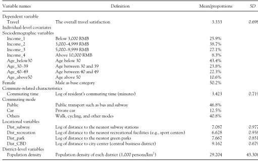
Table 2. Summarizing the travel satisfaction data used in the analysis

Variable names Definition Mean/proportions SD

Dependent variable

Travel The overall travel satisfaction 3.333 0.698 Individual-level covariates

Sociodemographic variables

Income_1 Below 3,000 RMB 25.9% Income_2 3,000–4,999 RMB 38.7% Income_3 5,000–9,999 RMB 27.1% Income_4 Above 10,000 RMB 8.3% Age_below30 Age below 30 43.4% Age_30–39 Age between 30 and 39 23.8% Age_40–49 Age between 40 and 49 22.3% Age_above50 Age above 50 10.6% Female Male as base category 50.2% Commute-related characteristics

Commuting time Log of resident’s commuting time (minutes) 3.423 0.719 Commuting mode

Public Public transport such as bus and subway 46.8%

Car Private car 12.5%

Others Walk, cycling, and other modes 40.8% Locational variables

Dist_subway Log of distance to the nearest subway stations 7.087 0.977 Dist_recreation Log of distance to the nearest recreational facilities (e.g., sport centers) 6.628 0.938 Dist_park Log of distance to the nearest green parks 7.667 0.851 Dist_CBD Log of distance to city center (central business district) 9.162 0.679 District-level variables

Population density Population density of each district (1,000 persons/km2) 29.204 43.306

Note:RMBDChinese Yuan Renminbi.

Figure 1. The histogram plot of the overall travel satisfaction superimposed with a density curve.

parks and subway stations, which are allowed to be dif-ferent in each geographical area. This is partly because spatial heterogeneity in the capitalization of access to green parks and subway stations into land values in the study area has been recently acknowledged (Harris, Dong, and Zhang 2013; Wu and Dong 2014). Moreover, although subway service expansion is cur-rently the focus of municipal policies for encouraging public transport in Beijing, a further exploration of spatially varying effects of proximity to subway stations could be beneficial to public transit development (e.g., identifying particular districts with transport infra-structure priority) and transport policy evaluation (Ma, Mitchell, and Heppenstall 2015).

Travel Satisfaction Model Specification

The empirical travel satisfaction equation to esti-mate is as follows:

Traveli,jDaX0 i,jCgL0i,j C dP0i,j CbjA0 i,j Cei,j

b_jDb_1;j;b_2;j0D½b1;b₂0C u1;j;u2;j

0

;

u »MVNð0;VÞ;e » MVN0;s2_eI; (25)

where Travel represents travel satisfaction;iandjare individual and district indexes as in Equation 1;X rep-resents sociodemographic variables including age, gen-der, and income (Table 2); L refers to locational variables of proximity to center city and recreational facilities whose effects are assumed to be fixed across districts; and P represents the urban form indicator (i.e., population density) at the district level. Parame-tersa,g, anddare fixed regression coefficients that we seek to estimate. Arefers to proximity to green parks and subway stations and b_j are the associated regres-sion coefficients that are assumed to be varied across districts. The fixed part (mean) ofb_jis [b1,b2] and the

random part is specified by [u1, u2], which follows a multivariate normal distribution with mean0and pre-cision matrix V. Different formations of the precision matrixVfrom nonspatial random slope MLM, MLM-MLCAR, and MLM-MICAR were discussed earlier.

Model Comparisons

Comparing the performance of nonspatial random slope MLM, MLM-MLCAR, and MLM-MICAR, we adopt two commonly used Bayesian procedures: the deviance information criterion (DIC; Spiegelhalter

et al. 2002) and the pseudo-Bayes factor (PsBF) calcu-lated by an approximation to marginal likelihoods of two competing models (Neelon, O’Malley, and Nor-mand 2010; Congdon 2014). The DIC is calculated as the sum of the posterior mean of the deviance (twice the negative log-likelihood of a model) and the num-ber of effective model parameters. As a rule of thumb, if two competing models differ in DIC by more than three, the model with smaller DIC is regarded as a bet-ter fitting (Spiegelhalbet-ter et al. 2002). The Bayes factor (BF), obtained as the ratio of marginal likelihoods for two models, is another popular way to compare two competing models, which provides the evidence in the data that favors one model relative to another (Kass and Raftery 1995).

Following Neelon, O’Malley, and Normand (2010), to overcome the great computational difficulties of BF (calculation of marginal likelihoods of a model), we use the PsBF—an approximation of the BF through a cross-validation estimate of the marginal likelihood of a model (Gelfand and Dey 1994) to compare the per-formance of different models. The cross-validation predictive density for observation i is expressed as (Neelon, O’Malley, and Normand 2010)

f yi;jjy½_¡ð Þi;j

D

Z

f yi;jju;y½_¡ð Þi;j

p.ujy_{½¡ð Þi;j}/du;

(26)

where y[-(i,j)] denotes the vector of outcome with the yi,j deleted and u represents the model parameters to estimate. The quantityf(yi,j|y[-(i,j)]) is called the

con-ditional predictive ordinate (CPO) for theith observa-tion in districtj, of which the Monte Carlo estimate is given by

d

CPOi;jDR=

X

r

1=f.yi;jjuð Þr/; (27)

where u(r) refers to the parameter vector sampled at the lth iteration l D 1, . . ., R (following a burn-in period) andf(yi,j|u(r)) is the likelihood of observation [i, j] evaluated at iterationl. The product of CPOs for each observation is called the pseudo-marginal likeli-hood (PsML; Gelfand and Dey 1994), and the ratio of PsMLs of two competing models gives a PsBF (Congdon 2014).

All competing models are coded using the R lan-guage. Diffuse or quite noninformative priors were

placed on model parameters: fixed regression

coefficients b » MVN (0, 1000*I18), the precision

matrix’»dwish(I2, 2), and the individual level

vari-ance se2 » IG (0.01, 0.01). Initial values for each

model parameter were drawn from their corresponding probability distribution. For each of these models, sta-tistical inferences were based on two MCMC chains, each of which consisted of 60,000 iterations with a burn-in period of 10,000. We further retained every tenth sample to reduce autocorrelation in each

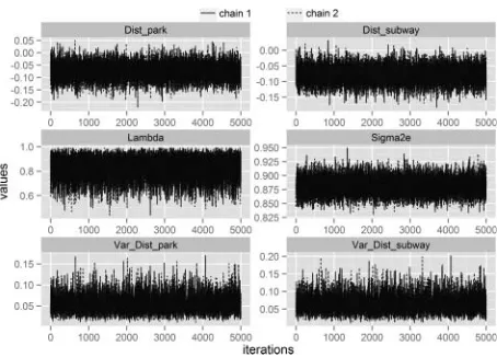
MCMC chain.1 MCMC diagnostics including trace

plots and Brooks–Gelman–Rubin scale reduction sta-tistics (Brooks and Gelman 1998) indicated rapid con-vergence of our samplers and efficient mixing of chains for each model under study. Figure 2 provides post-burn-in trace plots for several representative model parameters from MLM-MLCAR: fixed regres-sion coefficients including the proximity to nearest green park (Dist_park) and also the proximity to near-est subway station (Dist_subway), the individual-level variance parameter Sigma2e, the spatial correlation parameter λ, and variance parameters of two sets of random effects (Var_Dist_park and Var_Dist_sub-way). The two much overlapped trajectory lines show convergence and efficient mixing of chains (Figure 2). The mean of the lag-5 autocorrelations for parameters in MLM-MLCAR was 0.003, ranging from –0.026 to 0.063, and the 97.5 percent quantiles of the Brooks– Gelman–Rubin statistics were all less than 1.01, indi-cating good convergence of each chain (Neelon, O’Malley, and Normand 2010).

Model comparison results for the three models are provided in Table 3. All of the quantities are calcu-lated based on the 10,000 post-burn-in samples from

two MCMC chains. As shown in Table 3, the MLM-MLCAR produces the best model fit according to both the DIC and PsML statistics, compared to MLM-MICAR and nonspatial random slope MLM. Using the PsBF statistic, we find that the data strongly favor the MLM-MLCAR against nonspatial random slope MLM and MLM-MICAR with odds of 15.8 and 20.6, respectively (Kass and Raftery 1995). A better model fit of MLM-MLCAR against MLM-MICAR indicates the benefit of allowing the spatial correlation parame-ter to be estimated through data rather than defined a priori (equal to one in MLM-MICAR). The compari-son between nonspatial random slope MLM and MLM-MICAR also supports this argument.

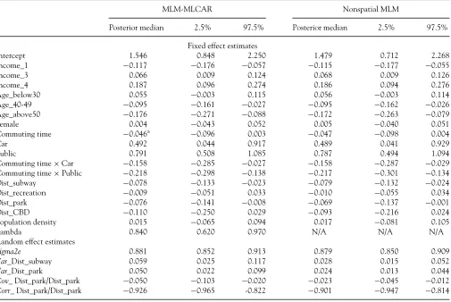
Results

Table 4 presents estimation results from MLM-MLCAR and nonspatial random slope MLM for a comparison. As shown later, posterior median and 95 percent credible intervals of each model parameter are produced. The estimate of the spatial correlation parameter in MLM-MLCAR is about 0.84 with a 95 percent credible interval [0.62, 0.97], indicating a fairly strong spatial dependence in each set of district-level random effects. We also investigate whether the district-level random effects of Dist_subway and Dis-t_park are spatially independent (as assumed to be so in nonspatial random slope MLM) by using the Moran’s I statistic based on the same spatial weights

matrix W used in MLM-MLCAR. The resultant

Moran coefficient for random effects of Dist_subway is 0.144 with ap value equal to<0.001, and the Moran

Table 3. Model fit comparisons using metrics of DIC, PsML, and PsBF

DIC PsML

PsBF (in favor of MLM-MLCAR)

MLM_MLCAR 17,602.0 –8,806.2 MLM_MICAR 17,608.7 –8,809.2 Nonspatial MLM 17,608.7 –8,809.0 MLM_MLCAR/

MLM_MICAR

–6.7 3.0 20.6 (strong)

MLM_MICAR/ nonspatial MLM

–6.7 2.8 15.8 (strong)

Note:DIC_D deviance information criterion; PsML_D pseudo-marginal likelihood; PsBF _D pseudo-Bayes factor; MLM _D multilevel modeling; MLCAR _D multivariate Leroux conditional autoregressive; MICAR_D multivariate intrinsic conditional autoregressive.

Figure 2. Trace plots based on two Markov chain Monte Carlo chains for six representative parameters from multilevel modeling-multivariate Leroux conditional autoregressive (MLM-MLCAR) model.

coefficient for random effects of Dist_park is 0.127 with ap value equal to<0.01. This demonstrates the existence of positive spatial dependence in the esti-mated random effects from nonspatial random slope MLM, which is in contradiction with the core model assumption of independence of random effects. Although there are no qualitative differences in fixed effect estimation between two models, MLM-MLCAR seems to be more efficient than nonspatial random slope MLM, as most of the 95 percent credible inter-vals of covariates are narrower than those from non-spatial random slope MLM.

Travel Satisfaction and Life Circumstance

The estimates from MLM-MLCAR demonstrate that most of these life circumstance variables are

sig-nificantly correlated with individuals’ travel

satisfaction (Table 4). For example, monthly income is significantly and positively associated with travel satisfaction. People with low-level income tend to have lower travel satisfaction, whereas high-level income tends to increase subjective travel satisfaction of residents. This broadly supports previous studies that have reported a significant impact of household income on life satisfaction or well-being, although the correlation is not linear (Easterlin 2001; Clark et al. 2008).

Distinctness is also found between different age cohorts. Older people are significantly associated with lower level of travel satisfaction, whereas young people (aged thirty and below) tend to score highest in satis-faction with travel. This is possibly because people aged forty and older are more likely to be involved in house-work (e.g., child care and family errands) and recrea-tional activities and thus they are more likely to be exposed to poor travel conditions in urban Beijing (Ma

Table 4. Summarizing the estimation results from the MLM-MICAR and MLM

MLM-MLCAR Nonspatial MLM

Posterior median 2.5% 97.5% Posterior median 2.5% 97.5%

Fixed effect estimates

Intercept 1.546 0.848 2.250 1.479 0.712 2.268 Income_1 ¡0.117 ¡0.176 ¡0.057 ¡0.115 ¡0.177 ¡0.055 Income_3 0.066 0.009 0.124 0.068 0.009 0.126 Income_4 0.187 0.096 0.274 0.186 0.094 0.276 Age_below30 0.055 ¡0.003 0.115 0.056 ¡0.003 0.114 Age_40-49 ¡0.095 ¡0.161 ¡0.027 ¡0.095 ¡0.162 ¡0.026 Age_above50 ¡0.176 ¡0.271 ¡0.088 ¡0.172 ¡0.263 ¡0.079 Female 0.004 ¡0.043 0.052 0.005 ¡0.040 0.051 Commuting time ¡0.046a ¡0.096 0.003 ¡0.047 ¡0.098 0.004 Car 0.492 0.044 0.917 0.489 0.041 0.929 Public 0.791 0.508 1.085 0.787 0.494 1.094 Commuting time£Car ¡0.158 ¡0.285 ¡0.027 ¡0.158 ¡0.287 ¡0.029 Commuting time£Public ¡0.218 ¡0.298 ¡0.138 ¡0.217 ¡0.301 ¡0.134 Dist_subway ¡0.078 ¡0.133 ¡0.023 ¡0.079 ¡0.132 ¡0.024 Dist_recreation ¡0.009 ¡0.051 0.033 ¡0.010 ¡0.055 0.034 Dist_park ¡0.076 ¡0.141 ¡0.008 ¡0.069 ¡0.137 ¡0.001 Dist_CBD ¡0.110 ¡0.250 0.029 ¡0.093 ¡0.216 0.024 Population density 0.015 ¡0.065 0.094 0.017 ¡0.081 0.105 Lambda 0.840 0.620 0.970 N/A N/A N/A Random effect estimates

Sigma2e 0.881 0.852 0.913 0.879 0.850 0.909 Var_Dist_subway 0.059 0.025 0.117 0.028 0.015 0.052 Var_Dist_park 0.050 0.022 0.099 0.024 0.013 0.044 Cov_ Dist_park/Dist_park ¡0.050 ¡0.103 ¡0.020 ¡0.023 ¡0.045 ¡0.012 Corr_ Dist_park/Dist_park ¡0.926 ¡0.965 -0.822 ¡0.901 ¡0.947 ¡0.814

Note:MLM_Dmultilevel modeling; MLCAR_Dmultivariate Leroux conditional autoregressive; CBD_Dcentral business district.

a_{Although the main effect of commuting time is not statistically significant at the 95 percent credible level, it is significant at the 90 percent credible level} with an interval of [–0.087, –0.005].

et al. 2014). Regarding the gender effect, there is no significant difference between men and women’s travel satisfaction, which is in line with prior studies reporting similar satisfaction for gender (e.g., Ettema et al. 2012).

Travel Satisfaction and Commuting Behavior

Commute to and from work accounts for an impor-tant part of daily life, and it has a significant and nega-tive effect on travel satisfaction. The MLM-MLCAR results show that with commuting time increasing, people’s satisfaction with travel decreases while every-thing else equal, and this association is significant at the 90 percent credible level (Table 4). Commuting mode is also very significantly correlated with overall travel satisfaction. Compared to other travel modes such as walking or cycling, people commuting by car or public transport (i.e., bus and subway) tend to have higher travel satisfaction. The relationship between commuting behavior and travel satisfaction is compli-cated, however, by the inclusion of interaction effects between commuting time and modes, which are all statistically significant in the model.

As shown in Table 4, the negative regression coeffi-cients of the interaction terms (Commuting time £ Car and Commuting time£Public) suggest that with commuting time increasing, people’s subjective satis-faction with travel by car and public transit tends to decrease. When commuting times for car or public transport surpass twenty-three or fifty-eight minutes, respectively, people’s travel satisfaction with car or public transport is lower than that with other commut-ing modes, such as walkcommut-ing or cyclcommut-ing.2 From our sur-vey data, we find that the average commuting time for the base category (e.g., walking and cycling) is approx-imately twenty minutes, which indicates that people are more likely to have higher satisfaction when they travel by car or public transport, rather than other commuting modes.

Travel Satisfaction and Geographical Context

The modeling results show that, of the locational variables, proximity to green parks and accessibility to subway stations are significantly associated with travel satisfaction. For instance, with close proximity to green parks at their residence, people tend to visit parks more often and they have higher travel satisfac-tion than their counterparts. Similarly, higher subway accessibility significantly increases residents’ travel

satisfaction, possibly due to the fact that the subway is fast, inexpensive, and uncongested in Beijing. People living in neighborhoods with higher population den-sity or proximity to various recreational facilities also have higher travel satisfaction, although their correla-tions are not significant at the 95 percent credible level. Although proximity to city center is usually con-sidered a proxy of employment accessibility, its corre-lation with travel satisfaction is insignificant. This is possibly because Beijing has undergone rapid urbaniza-tion, industrial decentralizaurbaniza-tion, and residential subur-banization since the 1990s. High-tech industry zones and housing were established mainly in the suburbs, whereas employment opportunities for tertiary indus-tries remained in the inner city (Ma et al. 2014). The emerging subcenters and coexistence of diversified land use configuration cause a complicated urban spa-tial structure in Beijing and also make it necessary to examine travel satisfaction under various geographical contexts.

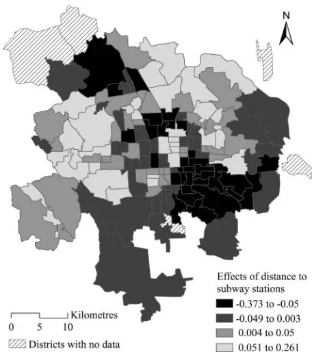
Regarding the random effect estimates of locational variables, Figure 3 illustrates the spatially varying effects of proximity to subway stations in urban Bei-jing. The break points in Figure 3 correspond to the lower quartile, median, and upper quartile of estimated posterior means of the district-level effect of proximity

Figure 3. District-level effects of proximity to subway stations using estimates from multilevel modeling-multivariate Leroux con-ditional autoregressive (MLM-MLCAR) model.

to subway stations. Clusters with large effects of being close to subway stations (large negatives) are identi-fied, including areas to the southeast of the central business district (CBD), areas near Zhongguancun (a subcenter in Beijing), and areas in the northwest sub-urb of Beijing. It suggests that increasing the subway accessibility, particularly for the districts around employment centers (e.g., the CBD and Zhongguan-cun) and large “bedroom” communities (e.g., Hui Long Guan in the northwest suburbs), will increase travel satisfaction of residents in these areas substan-tially. This is possibly because higher subway accessi-bility significantly increases commuting satisfaction on a typical workday, as a job–housing spatial mismatch exists in Beijing (Ma et al. 2014). This analysis, for the first time, investigates spatially varying effects of subway accessibility on travel satisfaction, identifies the particular districts with subway development prior-ities, and suggests useful solutions to improving peo-ple’s well-being in Beijing.

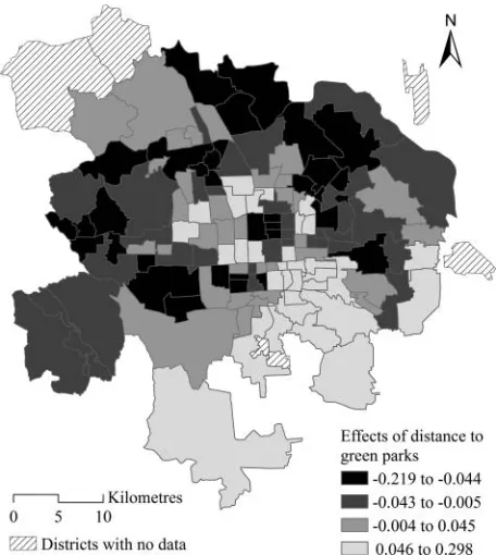
Figure 4 illustrates the spatially varying effects of proximity to green parks, with break points at the lower quartile, median, and upper quartile of estimated posterior means at the district level. It also shows that the marginal effect of proximity to green parks on travel satisfaction varies across districts, with the high

effect of proximity to green parks predominately dis-tributed in the northern area of Beijing. Although the employment subcenters are mostly located in northern Beijing, better access to green space substantially increases travel satisfaction of residents in northern districts, possibly due to the higher satisfaction with recreational travels. In addition, the random effect estimates of proximity to green parks and subway sta-tions from nonspatial random slope MLM and MLM-MLCAR are illustrated and compared in Figure 5, with a scatter plot superimposed by a 45-degree dashed line. By and large, it presents a good correspondence in estimates between these two models, with simple Pearson correlation coefficients for estimated effects of proximity to green parks and subway stations being 0.835 and 0.839, respectively. It also shows that the large positive effects of these two locational variables are reduced in MLM-MLCAR, whereas the small neg-ative values are raised.

Conclusion

This study presents a new modeling approach through the development of a spatial random slope MLM that incorporates the spatial dependence effects into standard nonspatial MLM. The motivation is that for many geographically clustered survey data, the cru-cial assumption of independence among the higher level spatial units underlying the standard nonspatial random slope MLM is challengeable. The geographical closeness of areal units is likely to induce spatial

Figure 5. Comparing effect estimates of proximity to green parks and subway stations from multilevel modeling-multivariate Leroux conditional autoregressive (MLM-MLCAR) and nonspatial multi-level modeling (MLM).

Figure 4. District-level effects of proximity to green parks using estimates from multilevel modeling-multivariate Leroux condi-tional autoregressive (MLM-MLCAR) model.

dependence in geographical-level random effects, which means that the contextual effects at higher level in random slope MLM might be dependent across space.

Building on an MCAR model, we define the area-level random effects as a complex and correlated spa-tial process, and propose a complex MLM-MLCAR approach. The proposed approach can simultaneously model the spatial dependence effect across space and the within-area correlations between different sets of random effects. Given the proliferation of geographi-cally grouped data on individuals and their extensive use in social, health, and environmental research, we anticipate that the developed approach could be useful in a wide range of applications.

Using Beijing as a case study, we use the new method to investigate the spatial variations of people’s subjective travel satisfaction and its determinants. Model results show that life circumstance variables including income and age and commute-related char-acteristics such as commuting time and travel mode choices are significantly associated with travel satisfac-tion. Regarding the locational variables, better access to subway stations and green parks is significantly cor-related with higher levels of travel satisfaction. Fur-thermore, the effects of proximity to subway stations and green parks exhibit a fairly strong spatial pattern in Beijing, with high and low values clustering together, respectively. This could be due to the rela-tively large spatial correlation parameter identified in the model.

One potential issue not addressed here regards the sensitivity of the identified district-level effect, due to the notable issue of uncertain geographic context (Kwan 2012). The problem might exist in our case study, as districts might not be the true geographical context that influences individuals’ subjective travel satisfaction. We hope, however, that using the devel-oped hybrid spatial MLM that allows the outcomes to be not only influenced by their immediate geographi-cal context but also by neighboring contexts, random effect estimates at the higher level can be more robust. Although spatial dependence is considered globally in our model, we find that some districts that are geo-graphical neighbors can have different random effect estimates (Figures 3 and 4). Our next step is to further incorporate a localized perspective of spatial depen-dence into the model using the approach developed by Lee and Mitchell (2013). A further extension of our method would allow for nonspatial dependence between aerial units. Pryce (2013), for example,

argued that Euclidean distance or contiguity might not be the only way that dependence occurs between aerial units—perceived substitutability; social net-works or communication and transport links might lead to some units being “close” even if they are spa-tially distant. In such circumstances, the conditional autoregressive component of the model could be con-structed in substitutability or network space rather than Cartesian space (ºaszkiewicz, Dong, and Harris 2014).

Acknowledgments

The authors are grateful for the comments of three reviewers and the editor, which have greatly improved the content of this article. They also would like to thank Professor Bill Browne and Dr. George Leckie from the Centre for Multilevel Modeling (CMM), University of Bristol for providing valuable comments on the previous draft of the article. Thanks are also due to Professor Wenzhong Zhang and Dr. Jianhui Yu from the Institute of Geographical Sciences and Natu-ral Resources Research, Chinese Academy of Sciences for providing the data used in the study.

Funding

This work was funded by the Economic and Social Research Council (ESRC) through the Applied Quan-titative Methods Network: Phase II, grant number ES/ K006460/1. The first author also gratefully acknowl-edges the ESRC for funding his doctoral research dur-ing 2011 and 2014 and support from the National Natural Science Foundation of China (Project No. 41201169).

Notes

1. For each of the spatial multilevel models implemented, the convergence of the MCMC sampler is diagnosed using the CODA package (Plummer et al. 2006) in R. In terms of efficient computation, a crucial part is updat-ing the spatially random effect, aJP by 1 (384 by 1 in this case) vector based on its full posterior conditional distribution. We take advantage of a desirable charac-teristic of the GMRFs, the sparsity of their precision matrix, and therefore some fast sparse matrix Cholesky factorization can be carried out. More specifically, a canonical parameterization of the posterior distribution of the spatial random effect is used to draw samples of them via a very useful and computationally efficient function in an R package, SPAM, created by Furrer and

Sain (2010). Details on fast sampling algorithms for GMRFs are provided in Rue and Held (2005) and Furrer and Sain (2010). It takes about four minutes for the MCMC sampler of the MLM-MLCAR model to pro-duce 10,000 samples on a laptop with an Intel Core 2.5 GHz processor. Before applying the code to the travel satisfaction data, we conducted a series of simula-tion studies with known data generating processes and using the geography (data structure) of the travel data to test the code. The results show that spatial multilevel models can accurately retrieve the true model parame-ters. The R code for implementing the spatial multilevel models and the simulation study results are available on request.

2. Based on estimates from MLM-MLCAR in Table 4, the marginal effects of commuting by car and public trans-ports (with other transport modes as baseline category) are 0.492 + (–0.158) £Commuting time and 0.791 + (–0.218) £ Commuting time, respectively. Equating the two marginal effects to zero (and exponentiating the solutions) gives the commuting time thresholds in the main text.

References

Anselin, L. 1988. Spatial econometrics: Methods and models. Dordrecht, The Netherlands: Kluwer Academic. Arcaya, M., M. Brewster, C. Zigler, and S. V. Subramanian.

2012. Area variations in health: A spatial multilevel modeling approach.Health and Place18:824–31. Assuncao, R. M. 2003. Space varying coefficient models for

small area data.Environmentrics14:453–73.

Ballas, D., and M. Tranmer. 2012. Happy people or happy place?: A multilevel modelling approach to the analysis of happiness and well-being.International Regional Sci-ence Review35:70–102.

Baltagi, B. H., B. Fingleton, and A. Pirotte. 2014. Spatial lag models with nested random effects: An instrumen-tal variable procedure with an application to English house prices.Journal of Urban Economics80:76–86. Banerjee, S., B. P. Carlin, and A. E. Gelfand. 2004.

Hierar-chical modeling and analysis for spatial data. Boca Raton, FL: Chapman and Hall/CRC.

Besag, J., J. C. York, and A. Mollie. 1991. Bayesian image resto-ration, with two principle applications in spatial statistics.

Annals of the Institute of Statistical Mathematics43:1–59. Brooks, S. P., and A. Gelman. 1998. General methods for

monitoring convergence of iterative simulations. Jour-nal of ComputatioJour-nal and Graphical Statistics7:434–55. Browne, W. J., and H. Goldstein. 2010. MCMC sampling

for a multilevel model with nonindependent residuals within and between cluster units.Journal of Educational and Behavioral Statistics35:453–73.

Browne, W. J., H. Goldstein, and J. Rasbash. 2001. Multi-ple-membership multiple-classification (MCMC) mod-els.Statistical Modelling1:103–24.

Chaix, B., J. Merlo, and P. Chauvin. 2005. Comparison of a spatial approach with the multilevel approach for investigating place effects on health: The example of healthcare utilisation in France.Journal of Epidemiology and Community Health59:517–26.

Chaix, B., J. Merlo, S. V. Subramanian, J. Lynch, and P. Chauvin. 2005. Comparison of a spatial perspective with the multilevel analytical approach in neighbor-hood studies: The case of mental and behavioural disor-ders due to psychoactive substance use in Malm€o, Sweden, 2001. American Journal of Epidemiology

162:171–82.

Chib, S., and E. Greenberg. 1995. Understanding the Metropolis–Hastings algorithm. The American Statisti-cian49:327–35.

Clark, A. E., E. Diener, Y. Georgellis, and R. E. Lucas. 2008. Lags and leads in life satisfaction: A test of the baseline hypothesis.The Economic Journal118:222–43.

Cliff, A., and J. K. Ord. 1981. Spatial processes: Models and applications.London: Pion.

Congdon, P. 2014. Applied Bayesian modeling. 2nd ed. Boca Raton, FL: Chapman & Hall/CRC.

Corrado, L., and B. Fingleton. 2012. Where is the econom-ics in spatial econometreconom-ics. Journal of Regional Sciences

52:210–39.

Cressie, N. 1993. Statistics for spatial data. Rev. ed. New York: Wiley.

Dong, G. P., and R. Harris. 2015. Spatial autoregressive models for geographically hierarchical data structures.

Geographical Analysis47:173–91.

Dong, G. P., R. Harris, K. Jones, and J. Yu. 2015. Multilevel modelling with spatial interaction effects with applica-tion to an emerging land market in Beijing, China.

PLoS ONE10 (6): e0130761.

Easterlin, R. A. 2001. Income and happiness: Towards a unified theory.The Economic Journal111:465–84. Ettema, D., M. Friman, T. Garling, L. E. Olsson, and S.

Fujii. 2012. How in-vehicle activities affect work commuters’ satisfaction with public transport. Journal of Transport Geography24:215–22.

Fotheringham, A. S., C. Brunsdon, and M. Charlton. 2002.

Geographically weighted regression: The analysis of spatially varying relationships. Chichester, UK: Wiley.

Furrer, R., and S. Sain. 2010. Spam: A sparse matrix R package with emphasis on MCMC methods for Gauss-ian Markov random fields.Journal of Statistical Software

36 (10): 1–25.

Gelfand, A. E. 2012. Hierarchical modeling for spatial data problems.Spatial Statistics1:30–39.

Gelfand, A. E., S. Banerjee, C. F. Sirmans, Y. Tu, and S. E. Ong. 2007. Multilevel modeling using spatial processes: Application to the Singapore housing market. Compu-tational Statistics and Data Analysis51:3567–79.

Gelfand, A. E., and D. Dey. 1994. Bayesian model choice: Asymptotics and exact calculations.Journal of the Royal Statistical Society: Series B56:501–14.

Gelfand, A. E., and P. Vounatsou. 2003. Proper multivariate conditional autoregressive models for spatial data anal-ysis.Biostatistics4:11–25.

Gelman, A., B. Carlin, H. S. Stern, and D. B. Rubin. 2004,

Bayesian Data Analysis, 2nd ed. Chapman & Hall/CRC. Goldstein, H. 2003. Multilevel statistical methods. 3rd ed.

London: Arnold.

Haining, R. 2003.Spatial data analysis: Theory and practice. Cambridge, UK: Cambridge University Press.

Harris, R., G. P. Dong, and W. Zhang. 2013. Using contex-tualized geographically weighted regression to model