GALILEO, University System of Georgia
GALILEO Open Learning Materials
Biological Sciences Open Textbooks Biological Sciences
Spring 2018
Introduction to Environmental Science: 2nd
Edition
Caralyn Zehnder
Georgia College and State University, [email protected] Kalina Manoylov
Georgia College and State University, [email protected] Samuel Mutiti
Georgia College and State University, [email protected] Christine Mutiti
Georgia College and State University, [email protected] Allison VandeVoort
Georgia College and State University, [email protected] See next page for additional authors
Follow this and additional works at:https://oer.galileo.usg.edu/biology-textbooks Part of theBiology Commons, and theEcology and Evolutionary Biology Commons
This Open Textbook is brought to you for free and open access by the Biological Sciences at GALILEO Open Learning Materials. It has been accepted for inclusion in Biological Sciences Open Textbooks by an authorized administrator of GALILEO Open Learning Materials. For more information, please [email protected].
Recommended Citation
Zehnder, Caralyn; Manoylov, Kalina; Mutiti, Samuel; Mutiti, Christine; VandeVoort, Allison; and Bennett, Donna, "Introduction to Environmental Science: 2nd Edition" (2018).Biological Sciences Open Textbooks. 4.
Authors
Caralyn Zehnder, Kalina Manoylov, Samuel Mutiti, Christine Mutiti, Allison VandeVoort, and Donna Bennett
Open Textbook
Georgia College and State University
UNIVERSITY SYSTEM OF GEORGIA
Caralyn Zehnder, Kalina Manoylov, Samuel Mutiti,
Christine Mutiti, Allison VandeVoort, Donna Bennett
Introduction to
Table of Contents
i.
Introduction
ii.
Population Ecology
iii.
Human Demography
iv.
Non-Renewable Energy
v.
Alternative Energy
vi.
Air Pollution
vii.
Climate Change
viii.
Water
Return to Table of Contents
Chapter 1: Introduction to Environmental Sciences
Learning Objectives
At the end of this section, students will be able to:
1. Describe, at an introductory level, the basic chemical and biological foundations of life on Earth
2. Define environment, ecosystems, and environmental sciences
3. Give examples of the interdisciplinary nature of environmental science 4. Define sustainability and sustainable development
5. Explain the complex relationship between natural and human systems, pertaining to environmental impact, the precautionary principle, and environmental justifications 6. Understand scientific approach and begin to apply the scientific method
The Chemical and Biological Foundations of Life
Elements in various combinations comprise all matter on Earth, including living things. Some of the most abundant elements in living organisms include carbon, hydrogen, nitrogen, oxygen, sulfur, and phosphorus. These form the nucleic acids, proteins, carbohydrates, and lipids that are the fundamental components of living matter. Biologists must understand these important building blocks and the unique structures of the atoms that make up molecules, allowing for the formation of cells, tissues, organ systems, and entire organisms.
At its most fundamental level, life is made up of matter. Matter is any substance that occupies space and has mass. Elements are unique forms of matter with specific chemical and physical properties that cannot be broken down into smaller substances by ordinary chemical reactions. There are 118 elements, but only 92 occur naturally. The remaining elements are synthesized in laboratories and are unstable. The five elements common to all living organisms are oxygen (O), carbon (C), hydrogen (H), and nitrogen (N) and phosphorous (P). In the non-living world, elements are found in different proportions, and some elements common to living organisms are relatively rare on the earth as a whole (Table 1.1). For example, the atmosphere is rich in nitrogen and oxygen but contains little carbon and hydrogen, while the earth’s crust, although it contains oxygen and a small amount of hydrogen, has little nitrogen and carbon. In spite of their differences in abundance, all elements and the chemical reactions between them obey the same chemical and physical laws regardless of whether they are a part of the living or non-living world.
Table 1.1. Approximate percentage of elements in living organisms (from bacteria to humans) compared to the non-living world. Trace represents less than 1%.
Biosphere Atmosphere Lithosphere
Oxygen (O) 65% 21% 46%
Carbon (C) 18% trace trace
Hydrogen (H) 10% trace trace
Nitrogen (N) 3% 78% trace
Phosphorus (P) trace trace >30%
The Structure of the Atom
An atom is the smallest unit of matter that retains all of the chemical properties of an element. For example, one gold atom has all of the properties of gold in that it is a solid metal at room temperature. A gold coin is simply a very large number of gold atoms molded into the shape of a coin and containing small amounts of other elements known as impurities. Gold atoms cannot be broken down into anything smaller while still retaining the properties of gold. An atom is
composed of two regions: the nucleus, which is in the center of the atom and contains protons and neutrons, and the outermost region of the atom which holds its electrons in orbit around the nucleus, as illustrated in Figure 1.1. Atoms contain protons, electrons, and neutrons, among other subatomic particles. The only exception is hydrogen (H), which is made of one proton and one electron with no neutrons.
Figure 1.1. Elements, such as helium, depicted here, are made up of atoms. Atoms are made up of protons and neutrons located within the nucleus, with electrons in orbitals surrounding the nucleus.
Protons and neutrons have approximately the same mass, about 1.67 × 10⁻²⁴ grams. Scientists arbitrarily define this amount of mass as one atomic mass unit (amu) (Table 1.2). Although similar in mass, protons and neutrons differ in their electric charge. A proton is positively
charged whereas a neutron is uncharged. Therefore, the number of neutrons in an atom contributes significantly to its mass, but not to its charge.
Table 1.2. Protons, neutrons, and electrons
Charge Mass (amu) Location in atom
Proton +1 1 Nucleus
Neutron 0 1 Nucleus
Electron -1 0 Orbitals
Electrons are much smaller in mass than protons, weighing only 9.11 × 10⁻²⁸ grams, or about 1/1800 of an atomic mass unit. Hence, they do not contribute much to an element’s overall atomic mass. Although not significant contributors to mass, electrons do contribute greatly to the atom’s charge, as each electron has a negative charge equal to the positive charge of a proton. In uncharged, neutral atoms, the number of electrons orbiting the nucleus is equal to the number of protons inside the nucleus. In these atoms, the positive and negative charges cancel each other out, leading to an atom with no net charge. Accounting for the sizes of protons, neutrons, and electrons, most of the volume of an atom—greater than 99 percent—is, in fact, empty space. With all this empty space, one might ask why so-called solid objects do not just pass through one another. The reason they do not is that the electrons that surround all atoms are negatively
charged and negative charges repel each other. When an atom gains or loses an electron, an ion is formed. Ions are charged forms of atoms. A positively charged ion, such as sodium (Na+), has lost one or more electrons. A negatively charged ion, such as chloride (Cl-), has gained one or more electrons.
Molecules
Molecules are formed when two or more atoms join together through chemical bonds to form a unit of matter. Throughout your study of environmental science, you will encounter many molecules including carbon dioxide gas. Its chemical formula is CO2, indicating that this molecule is made up of one carbon atom and two oxygen atoms. Some molecules are charged due to the ions they contain. This is the case for the nitrate (NO3-), a common source of nitrogen to plants. It contains one nitrogen atom and three oxygen atoms, and has an overall charge of negative one.
Isotopes
Isotopes are different forms of an element that have the same number of protons but a different number of neutrons. Some elements—such as carbon, potassium, and uranium—have naturally occurring isotopes. Carbon-12 contains six protons, six neutrons, and six electrons; therefore, it has a mass number of 12 (six protons and six neutrons). Carbon-14 contains six protons, eight neutrons, and six electrons; its atomic mass is 14 (six protons and eight electrons). These two alternate forms of carbon are isotopes. Some isotopes may emit neutrons, protons, and electrons,
and attain a more stable atomic configuration (lower level of potential energy); these are radioactive isotopes, or radioisotopes. Radioactive decay describes the energy loss that occurs when an unstable atom’s nucleus releases radiation, for example, carbon-14 losing neutrons to eventually become carbon-12.
Carbon
The basic functional unit of life is a cell and all organisms are made up of one or more cells. Cells are made of many complex molecules called macromolecules, such as proteins, nucleic acids (RNA and DNA), carbohydrates, and lipids. The macromolecules are a subset of organic molecules that are especially important for life. The fundamental component for all of these macromolecules is carbon. The carbon atom has unique properties that allow it to form covalent bonds with as many as four different atoms, making this versatile element ideal to serve as the basic structural component, or “backbone,” of the macromolecules.
Hydrocarbons
Hydrocarbons are organic molecules consisting entirely of carbon and hydrogen, such as methane (CH4. We often use hydrocarbons in our daily lives as fuels—like the propane in a gas grill or the butane in a lighter. The many covalent bonds between the atoms in hydrocarbons store a great amount of energy, which is released when these molecules are burned (oxidized). Methane, an excellent fuel, is the simplest hydrocarbon molecule, with a central carbon atom bonded to four different hydrogen atoms, as illustrated in Figure 1.2.
Figure 1.2. Methane (CH4) has a tetrahedral geometry, with each of the four hydrogen atoms spaced 109.5° apart.
As the backbone of the large molecules of living things, hydrocarbons may exist as linear carbon chains, carbon rings, or combinations of both. This three-dimensional shape or conformation of the large molecules of life (macromolecules) is critical to how they function.
Biological molecules
Life on Earth is primarily made up of four major classes of biological molecules, or biomolecules. These include carbohydrates, lipids, proteins, and nucleic acids.
Most people are familiar with carbohydrates, one type of macromolecule, especially when it comes to what we eat. Carbohydrates are, in fact, an essential part of our diet; grains, fruits, and vegetables are all natural sources of carbohydrates. Carbohydrates provide energy to the body, particularly through glucose, a simple sugar that is a component of starch and an ingredient in many staple foods. Carbohydrates also have other important functions in humans, animals, and plants. Carbohydrates can be represented by the stoichiometric formula (CH2O)n, where n is the number of carbons in the molecule. In other words, the ratio of carbon to hydrogen to oxygen is 1:2:1 in carbohydrate molecules. This formula also explains the origin of the term
“carbohydrate”: the components are carbon (“carbo”) and the components of water (hence, “hydrate”). The chemical formula for glucose is C6H12O6. In humans, glucose is an important source of energy.
During cellular respiration, energy is released from glucose, and that energy is used to help make adenosine triphosphate (ATP). Plants synthesize glucose using carbon dioxide and water, and glucose in turn is used for energy requirements for the plant. Excess glucose is often stored as starch that is catabolized (the breakdown of larger molecules by cells) by humans and other animals that feed on plants. Plants are able to synthesize glucose, and the excess glucose, beyond the plant’s immediate energy needs, is stored as starch in different plant parts, including roots and seeds. The starch in the seeds provides food for the embryo as it germinates and can also act as a source of food for humans and animals.
Lipids include a diverse group of compounds such as fats, oils, waxes, phospholipids, and steroids that are largely nonpolar in nature. Nonpolar molecules are hydrophobic (“water
fearing”), or insoluble in water. These lipids have important roles in energy storage, as well as in the building of cell membranes throughout the body.
Proteins are one of the most abundant organic molecules in living systems and have the most diverse range of functions of all macromolecules. Proteins may be structural, regulatory, contractile, or protective; they may serve in transport, storage, or membranes; or they may be toxins or enzymes. Each cell in a living system may contain thousands of proteins, each with a unique function. Their structures, like their functions, vary greatly.
Enzymes, which are produced by living cells, speed up biochemical reactions (like digestion) and are usually complex proteins. Each enzyme has a specific shape or formation based on its use. The enzyme may help in breakdown, rearrangement, or synthesis reactions.
Proteins have different shapes and molecular weights. Protein shape is critical to its function, and many different types of chemical bonds maintain this shape. Changes in temperature, pH, and exposure to chemicals may cause a protein to denature. This is a permanent change in the shape of the protein, leading to loss of function. All proteins are made up of different arrangements of the same 20 types of amino acids. These amino acids are the units that make up proteins. Ten of these are considered essential amino acids in humans because the human body cannot produce them and they are obtained from the diet. The sequence and the number of amino acids
ultimately determine the protein's shape, size, and function.
Nucleic acids are the most important macromolecules for the continuity of life. They carry the genetic blueprint of a cell and carry instructions for the functioning of the cell. The two main types of nucleic acids are deoxyribonucleic acid (DNA) and ribonucleic acid (RNA). DNA is the genetic material found in all living organisms, ranging from single-celled bacteria to
multicellular mammals. DNA controls all of the cellular activities by turning the genes “on” or “off.” The other type of nucleic acid, RNA, is mostly involved in protein synthesis.
DNA has a double-helix structure (Figure 1.3).
Figure 1.3. Native DNA is an antiparallel double helix. The phosphate backbone (indicated by the curvy lines) is on the outside, and the bases are on the inside. Each base from one strand interacts via hydrogen bonding with a base from the opposing strand. (credit: Jerome Walker/Dennis Myts)
Biological organization
All living things are made of cells; the cell itself is the smallest fundamental unit of structure and function in living organisms. In most organisms, these cells contain organelles, which provide specific functions for the cell. Living organisms have the following properties: all are highly organized, all require energy for maintenance and growth, and all grow over time and respond to their environment. All organisms adapt to the environment and all ultimately reproduce
contributing genes to the next generation. Some organisms consist of a single cell and others are multicellular. Organisms are individual living entities. For example, each tree in a forest is an organism.
All the individuals of a species living within a specific area are collectively called a population. Populations fluctuate based on a number of factors: seasonal and yearly changes in the
environment, natural disasters such as forest fires and volcanic eruptions, and competition for resources between and within species. A community is the sum of populations inhabiting a particular area. For instance, all of the trees, insects, and other populations in a forest form the forest’s community. The forest itself is an ecosystem.
An ecosystem consists of all the living things in a particular area together with the abiotic, non-living parts of that environment such as nitrogen in the soil or rain water. At the highest level of organization, the biosphere is the collection of all ecosystems, and it represents the zones of life on earth. It includes land, water, and even the atmosphere to a certain extent.
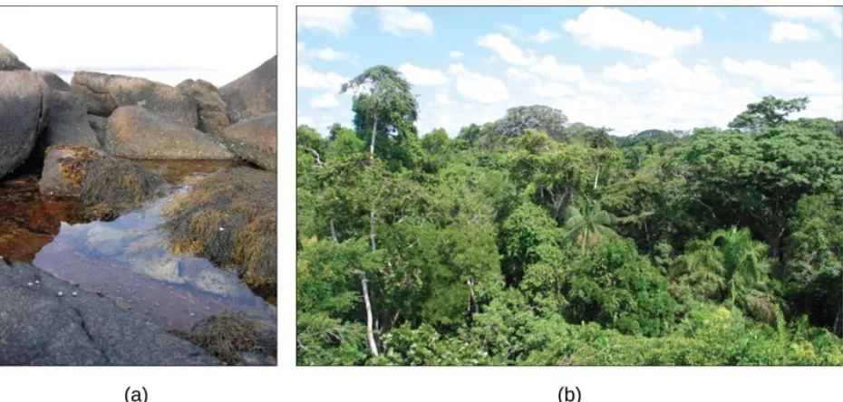
Life in an ecosystem is often about competition for limited resources, a characteristic of the process of natural selection. Competition in communities (all living things within specific habitats) is observed both within species and among different species. The resources for which organisms compete include organic material from living or previously living organisms, sunlight, and mineral nutrients, which provide the energy for living processes and the matter to make up organisms’ physical structures. Other critical factors influencing community dynamics are the components of its physical and geographic environment: a habitat’s latitude, amount of rainfall, topography (elevation), and available species. These are all important environmental variables that determine which organisms can exist within a particular area. Ecosystems can be small, such as the tidal pools found near the rocky shores of many oceans, or large, such as the Amazon Rainforest in Brazil (Figure 1.4).
There are three broad categories of ecosystems based on their general environment: freshwater, ocean water (marine), and terrestrial. Within these broad categories are individual ecosystem types based on the organisms present and the type of environmental habitat. Ocean ecosystems are the most common, comprising 75 percent of the Earth's surface. The shallow ocean
ecosystems include extremely biodiverse coral reef ecosystems, and the deep ocean surface is known for its large numbers of plankton and krill (small crustaceans) that support it. These two
environments are especially important to aerobic respirators worldwide as the phytoplankton perform 40 percent of all photosynthesis on Earth. Although not as diverse as the other two, deep ocean ecosystems contain a wide variety of marine organisms. Such ecosystems exist even at the bottom of the ocean where light is unable to penetrate through the water.
Freshwater ecosystems are the rarest, occurring on only 1.8 percent of the Earth's surface. Lakes, rivers, streams, and springs comprise these systems; they are quite diverse, and they support a variety of fish, amphibians, reptiles, insects, phytoplankton, fungi, and bacteria.
Figure 1.4. (a) A tidal pool ecosystem in Matinicus Island, Maine, is a small ecosystem, while (b) the Amazon rainforest in Brazil is a large ecosystem. (credit a: modification of work by Jim Kuhn; credit b: modification of work by Ivan Mlinaric)
Terrestrial ecosystems, also known for their diversity, are grouped into large categories called biomes, such as tropical rainforests, savannas, deserts, coniferous forests, deciduous forests, and tundra. Grouping these ecosystems into just a few biome categories obscures the great diversity of the individual ecosystems within them. For example, there is great variation in desert
vegetation: the saguaro cacti and other plant life in the Sonoran Desert, in the United States, are relatively abundant compared to the desolate rocky desert of Boa Vista, an island off the coast of Western Africa.
All living things require energy in one form or another. It is important to understand how organisms acquire energy and how that energy is passed from one organism to another through food webs. Food webs illustrate how energy flows directionally through ecosystems, including how efficiently organisms acquire it, use it, and how much remains for use by other organisms of
[image:12.612.75.540.212.434.2]
the food web. The flow of energy and matter through the ecosystems influences the abundance and distribution of organisms within them.
Ecosystems are complex with many interacting parts. They are routinely exposed to various disturbances: changes in the environment that affect their compositions, such as yearly variations in rainfall and temperature. Many disturbances are a result of natural processes. For example, when lightning causes a forest fire and destroys part of a forest ecosystem, the ground is eventually populated with grasses, followed by bushes and shrubs, and later mature trees: thus, the forest is restored to its former state. This process is so universal that ecologists have given it a name—succession. The impact of environmental disturbances caused by human activities is now as significant as the changes wrought by natural processes. Human agricultural practices, air pollution, acid rain, global deforestation, overfishing, oil spills, and illegal dumping on land and into the ocean all have impacts on ecosystems.
We rely on ecosystem services. Earth’s natural systems provide ecosystem services required for our survival such as: air and water purification, climate regulation, and plant pollination. We have degraded nature’s ability to provide these services by depleting resources, destroying habitats, and generating pollution. The benefits people obtain from ecosystems include: nutrient cycling, soil formation, and primary production. Another important service of natural
ecosystems is provisioning like food production, production of wood, fibers and fuel. Ecosystems are responsible for climate regulation, flood regulation together with disease
regulation. Finally ecosystems provide cultural and esthetic services. As humans we benefit from observing natural habitats, recreation in waters and mountains. Nature is a source of inspiration for poets and writers. It is a source of aesthetic, religious and other nonmaterial benefits.
Studying ecosystem structure in its original state is the only way we can make anthropogenic (man-made) systems like agricultural fields, reservoirs, fracking operations, and dammed rivers work for human benefit with minimal impact on our and other organisms’ health.
Environment and environmental science
Viewed from space, Earth (Figure 1.5) offers no clues about the diversity of lifeforms that reside there. The first forms of life on Earth are thought to have been microorganisms that existed for billions of years in the ocean before plants and animals appeared. The mammals, birds, and plants so familiar to us are all relatively recent, originating 130 to 200 million years ago. Humans have inhabited this planet for only the last 2.5 million years, and only in the last 200,000 years have humans started looking like we do today. There are around 7.35 billion people today (https://www.census.gov/popclock/).
[image:14.612.102.494.72.279.2]
Figure 1.5 This NASA image is a composite of several satellite-based views of Earth. To make the whole-Earth image, NASA scientists combine observations of different parts of the planet. (credit: NASA/GSFC/NOAA/USGS)
The word environment describes living and nonliving surroundings relevant to organisms. It incorporates physical, chemical and biological factors and processes that determine the growth and survival of organisms, populations, and communities. All these components fit within the ecosystem concept as a way to organize all of the factors and processes that make up the environment. The ecosystem includes organisms and their environment within a specific area. Review the previous section for in-depth information regarding the Earth’s ecosystems. Today, human activities influence all of the Earth’s ecosystems.
Environmental science studies all aspects of the environment in an interdisciplinary way. This means that it requires the knowledge of various other subjects including biology, chemistry, physics, statistics, microbiology, biochemistry, geology, economics, law, sociology, etc. It is a relatively new field of study that has evolved from integrated use of many disciplines.
Environmental engineering is one of the fastest growing and most complex disciplines of engineering. Environmental engineers solve problems and design systems using knowledge of environmental concepts and ecology, thereby providing solutions to various environmental problems. Environmentalism, in contrast, is a social movement through which citizens are involved in activism to further the protection of environmental landmarks and natural resources. This is not a field of science, but incorporates some aspects of environmental knowledge to advance conservation and sustainability efforts.
The Process of Science
Environmental science is a science, but what exactly is science? Science (from the Latin scientia, meaning “knowledge”) can be defined as all of the fields of study that attempt to comprehend the nature of the universe and all its parts. The scientific method is a method of research with defined steps that include experiments and careful observation. One of the most important aspects of this method is the testing of hypotheses by means of repeatable experiments. A
hypothesis is a suggested explanation for an event, which can be tested. A theory is a tested and confirmed explanation for observations or phenomena that is supported by many repeated
experiences and observations.
The scientific method
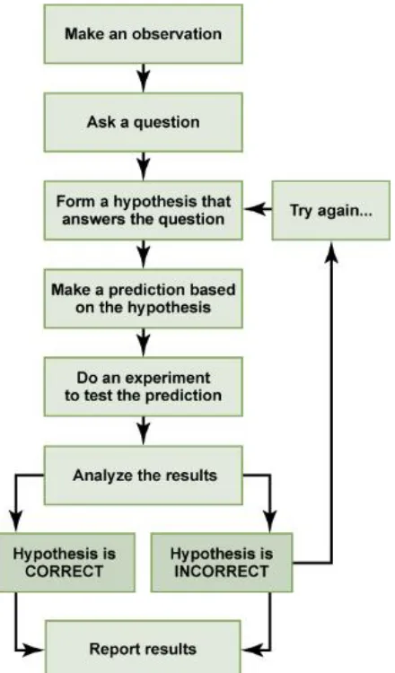
The scientific process typically starts with an observation (often a problem to be solved) that leads to a question. The scientific method consists of a series of well-defined steps. If a
hypothesis is not supported by experimental data, a new hypothesis can be proposed. Let’s think about a simple problem that starts with an observation and apply the scientific method to solve the problem. One Monday morning, a student arrives in class and quickly discovers that the classroom is too warm. That is an observation that also describes a problem: the classroom is too warm. The student then asks a question: “Why is the classroom so warm?”
Proposing a Hypothesis
Recall that a hypothesis is a suggested explanation that can be tested. To solve a problem, several hypotheses may be proposed. For example, one hypothesis might be, “The classroom is warm because no one turned on the air conditioning.” But there could be other responses to the
question, and therefore other hypotheses may be proposed. A second hypothesis might be, “The classroom is warm because there is a power failure, and so the air conditioning doesn’t work.” Once a hypothesis has been selected, the student can make a prediction. A prediction is similar to a hypothesis but it typically has the format “If . . . then . . . .” For example, the prediction for the first hypothesis might be, “If the student turns on the air conditioning, then the classroom will no longer be too warm.”
Testing a Hypothesis
A valid hypothesis must be testable. It should also be falsifiable, meaning that it can be disproven by experimental results. Importantly, science does not claim to “prove” anything because scientific understandings are always subject to modification with further information. This step — openness to disproving ideas — is what distinguishes sciences from non-sciences. The presence of the supernatural, for instance, is neither testable nor falsifiable.
To test a hypothesis, a researcher will conduct one or more experiments designed to eliminate, or disprove, the hypotheses. Each experiment will have one or more variables and one or more controls. A variable is any part of the experiment that can vary or change during the experiment. The independent variable is the variable that is manipulated throughout the course of the
experiment. The dependent variable, or response variable is the variable by which we measure change in response to the independent variable. Ideally, all changes that we measure in the dependent variable are because of the manipulations we made to the independent variable. In most experiments, we will maintain one group that has had no experimental change made to it. This is the control group. It contains every feature of the experimental group except it is not given any manipulation. Therefore, if the results of the experimental group differ from the control group, the difference must be due to the hypothesized manipulation, rather than some outside factor. Look for the variables and controls in the examples that follow.
To test the hypothesis “The classroom is warm because no one turned on the air conditioning,” the student would find out if the air conditioning is on. If the air conditioning is turned on but does not work, there should be another reason, and this hypothesis should be rejected. To test the second hypothesis, the student could check if the lights in the classroom are functional. If so, there is no power failure and this hypothesis should be rejected. Each hypothesis should be tested by carrying out appropriate experiments. Be aware that rejecting one hypothesis does not
determine whether or not the other hypotheses can be accepted; it simply eliminates one hypothesis that is not valid (Figure 1.7). Using the scientific method, the hypotheses that are inconsistent with experimental data are rejected.
The scientific method may seem too rigid and structured. It is important to keep in mind that, although scientists often follow this sequence, there is flexibility. Sometimes an experiment leads to conclusions that favor a change in approach; often, an experiment brings entirely new
scientific questions to the puzzle. Many times, science does not operate in a linear fashion; instead, scientists continually draw inferences and make generalizations, finding patterns as their research proceeds. Scientific reasoning is more complex than the scientific method alone
suggests. Notice, too, that the scientific method can be applied to solving problems that aren’t necessarily scientific in nature.
Figure 1.7. The scientific method consists of a series of well-defined steps. If a hypothesis is not supported by experimental data, a new hypothesis can be proposed.
Sustainability and Sustainable Development
In 1983 the United Nations General Assembly passed a resolution that established the Special Commission on the Environmental Perspective to the Year 2000 and Beyond
(http://www.un.org/documents/ga/res/38/a38r161.htm). Their charge was:
a. To propose long-term environmental strategies for achieving sustainable development to the year 2000 and beyond;
b. To recommend ways in which concern for the environment may be translated into greater co-operation among developing countries and between countries at different stages of economic and social development and lead to the achievement of common and mutually supportive objectives which take account of the interrelationships between people, resources, environment and development;
c. To consider ways and means by which the international community can deal more effectively with environmental concerns, in light of the other recommendations in its report;
d. To help define shared perceptions of long-term environmental issues and of the appropriate efforts needed to deal successfully with the problems of protecting and enhancing the environment, a long-term agenda for action during the coming decades, and aspirational goals for the world community, taking into account the relevant resolutions of the session of a special character of the Governing Council in 1982.
Although the report did not technically invent the term sustainability, it was the first credible and widely disseminated study that used this term in the context of the global impacts of humans on the environment. Its main and often quoted definition refers to sustainable development as development that meets the needs of the present without compromising the ability of future generations to meet their own needs. The report uses the terms ‘sustainable development’, ‘sustainable’, and ‘sustainability’ interchangeably, emphasizing the connections among social equity, economic productivity, and environmental quality (Figure 1.6). This three-pronged approach to sustainability is now commonly referred to as the triple bottom-line. Preserving the environment for humans today and in the future is a responsibility of every generation and a long-term global goal. Sustainability and the triple bottom-line (meeting environmental, economic, and social goals simultaneously) require that we limit our environmental impact, while promoting economic well-being and social equity.
Figure 1.6. A depiction of the sustainability paradigm in terms of its three main components, showing various intersections among them. Source: International Union for the Conservation of Nature.
Examples of sustainable development include sustainable agriculture, which is agriculture that does not deplete soils faster than they form and does not destroy the biodiversity of the area. Sustainable farming and ranching do not reduce the amount of healthy soil, clean water, genetic diversity of crop plants and animals. Maintaining as much ecological biodiversity as possible in the agro-ecosystem is essential to long-term crop and livestock production.
The IPAT Equation
As attractive as the concept of sustainability may be as a means of framing our thoughts and goals, its definition is rather broad and difficult to work with when confronted with choices among specific courses of action. One way of measuring progress toward achieving sustainable goals can be with the application of the IPAT equation. This equation was designed in an attempt to define the different ways that a variety of factors contribute to the environmental degradation, or impact, of a particular setting. Importantly, IPAT tells us that there are more ways we impact our environment than just through pollution:
I = P x A x T
I represents the impacts on an environment P is the size of the relevant human population A is the affluence of the population
T is the technology available to the population
Affluence, or wealth, tells us the level of consumption per person. Wealthy societies consume more goods and services per person. Because of this, their environmental impact is multiplied. Technology, or impact per unit of consumption, interpreted in its broadest sense. This includes any human-created tool, system, or organization designed to enhance efficiency. As societies gain greater access to technology, they are able to do more work with fewer individuals. This equates to a greater impact per person. While this equation is not meant to be mathematically rigorous, it provides a way of organizing information for analysis.
The proportion of people living in cities has greatly increased over the past 50 years. We can use the IPAT equation to estimate the impact of these urban populations. When the impact of
technology, which is much easier to access in urban settings, is combined with the impact of population, the impact on the environment is multiplied. In an increasingly urban world, we must focus much of our attention on the environments of cities and on the effects of cities on the rest of the environment. This equation also has large-scale applications in the environmental
sciences, and was included in the Intergovernmental Panel on Climate Change Special Report on Emissions Scenarios (2001) to project future greenhouse gas emissions across the globe.
The precautionary principle
The precautionary principle or the precautionary approach is one perspective of environmental risk management. The precautionary principle stakes that “When the health of humans and the environment is at stake, it may not be necessary to wait for scientific certainty to take protective action”. In other words, better to be safe than sorry. Proponents of the precautionary principle also believe that the burden of proof should be on the individual, company or government who is proposing the action, not on the people who will be affected by it. For example, if environmental regulations concerning pesticides were based on the precautionary principle (in the United States, they are not), then any pesticide that could potentially harm the environment or human health would not be used. Overuse of the precautionary principle can have negative
consequences as well. If federal regulations concerning medicines for human use were based on the precautionary principle (again, in the United States, they are not), then any medicine that could potentially harm any person would not be used. This would effectively ban nearly all medical trials leading to new medications.
What is the environment worth to you?
The environment, and its benefits to individuals or groups, can be viewed and justified from multiple perspectives. A utilitarian justification for environmental conservation means that we should protect the environment because doing so provides a direct economic benefit to people. For example, someone might propose not developing Georgia’s coastal salt marshes because the young of many commercial fishes live in salt marshes and the fishers will collapse without this habitat. An ecological justification for environmental conservation means that we should protect the environmental because doing so will protect both species that are beneficial to other as well as other species and an ecological justification for conservation acknowledges the many
ecosystem services that we derive from healthy ecosystems. For example, we should protect Georgia’s coastal salt marshes because salt marshes purify water, salt marshes are vital to the survival of many marine fishes and salt marshes protect our coasts from storm surges. An aesthetic justification for conservation acknowledges that many people enjoy the outdoors and do not want to live in a world without wilderness. One could also think of this as recreational, inspirational, or spiritual justification for conservation. For example, salt marshes are beautiful places and I always feel relaxed and calm when I am visiting one, therefore we should protect salt marches. And finally a moral justification represents the belief that various aspects of the environment have a right to exist and that it is our moral obligation to allow them to continue or help them persist. Someone who was arguing for conservation using a moral justification would say that it is wrong to destroy the coastal salt marshes.
_____________________________________________________________________________ Global perspective
The solution to most environmental problems requires a global perspective. Human population size has now reached a scale where the environmental impacts are global in scale and will require multilateral solutions. You will notice this theme continue as you move through the next seven chapters of this text. As you do so, keep in mind that the set of environmental, regulatory, and economic circumstances common in the United States are not constant throughout the world. Be ready to investigate environmental situations and problems from a diverse set of viewpoints throughout this semester.
Parts of this chapter have been modified from the OpenStax textbooks.
Study questions
1. Why there was a need to study the impact of human population growth on the environment?
2. What does sustainability mean to you?
3. What are the consequences of unsustainable vs. sustainable living? What impacts do these have on quality of life do we want for us and future generations?
4. Think of an environmental problem that requires a global perspective for a solution. How might this problem be examined from a variety of environmental justification
perspectives?
Websites for more information and further discussion
Information about the field of environmental science: http://www.environmentalscience.org/
"Process" of science http://undsci.berkeley.edu/
ReturntoTableofContents
Chapter
2:
Population
Ecology
A population of elephants at Pinnewala Elephant Orphanage, Sri
Lanka. Photo by Paginazero, Wikimedia commons. A shoal of anchovies in Liguria, Italy. Photo by Alessandro Duci. Wikimedia commons.
Learning Outcomes - At the end of this, chapter students will be able to:
• Define the variables in the exponential and logistic growth equations. • Use the exponential and logistic equations to predict population growth rate.
• Compare the environmental conditions represented by the exponential growth model vs. the logistic
growth model.
• Define carrying capacity and be able to label the carrying capacity on a graph.
• Compare density-dependent and density-independent factors that limit population growth and give
examples of each.
• Interpret survivorship curves and give examples of organisms that would fit each type of curve.
Chapter outline
2.1 Population Ecology... 2 2.2 Population Growth Models ... 2 2.2.1 Exponential Growth ... 2 2.2.2 Logistic Growth ... 4 2.3 Factors limiting population growth... 7 2.4 Life Tables and Survivorship... 9
2.1 Population Ecology
Ecology is a sub-discipline of biology that studies the interactions between organisms and their environments. A group of interbreeding individuals (individuals of the same species) living and interacting in a given area at a given time is defined as a population. These individuals rely on the same resources and are influenced by the same environmental factors. Population ecology, therefore, is the study of how individuals of a particular species interact with their environment and change over time. The study of any population usually begins by determining how many individuals of a particular species exist, and how closely associated they are with each other. Within a particular habitat, a
population can be characterized by its population size (N), defined by the total number of individuals, and its population density, the number of individuals of a particular species within a specific area or volume (units are number of individuals/unit area or unit volume). Population size and density are the two main characteristics used to describe a population. For example, larger populations may be more stable and able to persist better than smaller populations because of the greater amount of genetic variability, and their potential to adapt to the environment or to changes in the environment. On the other hand, a member of a population with low population density (more spread out in the habitat), might have more difficulty finding a mate to reproduce compared to a population of higher density. Other characteristics of a population include dispersion – the way individuals are spaced within the area; age structure – number of individuals in different age groups and; sex ratio – proportion of males to females; and growth – change in population size (increase or decrease) over time.
2.2 Population Growth Models
Populations change over time and space as individuals are born or immigrate (arrive from outside the population) into an area and others die or emigrate (depart from the population to another location). Populations grow and shrink and the age and gender composition also change through time and in response to changing environmental conditions. Some populations, for example trees in a mature forest, are relatively constant over time while others change rapidly. Using idealized models, population ecologists can predict how the size of a particular population will change over time under different conditions.
2.2.1 ExponentialGrowth
Charles Darwin, in his theory of natural selection, was greatly influenced by the English clergyman Thomas Malthus. Malthus published a book (An Essay on the Principle of Population) in 1798 stating that populations with unlimited natural resources grow very rapidly. According to the Malthus’ model, once population size exceeds available resources, population growth decreases dramatically. This accelerating pattern of increasing population size is called exponential growth, meaning that the population is increasing by a fixed percentage each year. When plotted (visualized) on a graph showing how the population size increases over time, the result is a J-shaped curve (Figure 2.1). Each individual in the population reproduces by a certain amount (r) and as the population gets larger, there are more individuals reproducing by that same amount (the fixed percentage). In nature, exponential growth only occurs if there are no external limits.
One example of exponential growth is seen in bacteria. Bacteria are prokaryotes (organisms whose cells lack a nucleus and membrane-bound organelles) that reproduce by fission (each individual cell splits into two new cells). This process takes about an hour for many bacterial species. If 100 bacteria are placed in a large flask with an unlimited supply of nutrients (so the nutrients will not
become depleted), after an hour, there is one round of division and each organism divides, resulting in 200 organisms - an increase of 100. In another hour, each of the 200 organisms divides, producing 400 - an increase of 200 organisms. After the third hour, there should be 800 bacteria in the flask - an increase of 400 organisms. After ½ a day and 12 of these cycles, the population would have increased from 100 cells to more than 24,000 cells. When the population size, N, is plotted over time, a J-shaped growth curve is produced (Figure 2.1). This shows that the number of individuals added during each reproduction generation is accelerating – increasing at a faster rate.
Figure 2.1: The “J” shaped curve of exponential growth for a hypothetical population of bacteria. The
population starts out with 100 individuals and after 11 hours there are over 24,000 individuals. As time goes on and the population size increases, the rate of increase also increases (each step up becomes bigger). In this figure “r” is positive.
This type of growth can be represented using a mathematical function known as the exponential growth model:
G = r x N (also expressed as dN/dt = r x N). In this equation
G (or dN/dt) is the population growth rate, it is a measure of the number of individuals added per time interval time.
r is the per capita rate of increase (the average contribution of each member in a population to population growth; per capita means “per person”).
N is the population size, the number of individuals in the population at a particular time.
Percapitarateofincrease(r)
In exponential growth, the population growth rate (G) depends on population size (N) and the per capita rate of increase (r). In this model r does not change (fixed percentage) and change in population growth rate, G, is due to change in population size, N. As new individuals are added to the population, each of the new additions contribute to population growth at the same rate (r) as the individuals already in the population.
r = (birth rate + immigration rate) – (death rate and emigration rate).
If r is positive (> zero), the population is increasing in size; this means that the birth and immigration rates are greater than death and emigration.
If r is negative (< zero), the population is decreasing in size; this means that the birth and immigration rates are less than death and emigration rates.
If r is zero, then the population growth rate (G) is zero and population size is unchanging, a condition known as zero population growth. “r” varies depending on the type of organism, for example a population of bacteria would have a much higher “r” than an elephant population. In the exponential growth model r is multiplied by the population size, N, so population growth rate is largely influenced by N. This means that if two populations have the same per capita rate of increase (r), the population with a larger N will have a larger population growth rate than the one with a smaller
N.
2.2.2 LogisticGrowth
Exponential growth cannot continue forever because resources (food, water, shelter) will become limited. Exponential growth may occur in environments where there are few individuals and plentiful resources, but soon or later, the population gets large enough that individuals run out of vital resources such as food or living space, slowing the growth rate. When resources are limited,
populations exhibit logistic growth. In logistic growth a population grows nearly exponentially at first when the population is small and resources are plentiful but growth rate slows down as the population size nears limit of the environment and resources begin to be in short supply and finally stabilizes (zero population growth rate) at the maximum population size that can be supported by the environment (carrying capacity). This results in a characteristic S-shaped growth curve (Figure 2.2). The mathematical function or logistic growth model is represented by the following equation:
�
=
�
∗
�
∗
[
�
−
�
�
]
Where,K is the carrying capacity – the maximum population size that a particular environment can sustain (“carry”). Notice that this model is similar to the exponential growth model except for the addition of the carrying capacity.
In the exponential growth model, population growth rate was mainly dependent on N so that each new individual added to the population contributed equally to its growth as those individuals previously in the population because per capita rate of increase is fixed. In the logistic growth model, individuals’ contribution to population growth rate depends on the amount of resources available (K). As the number of individuals (N) in a population increases, fewer resources are available to each
[image:27.612.62.508.103.375.2]
individual. As resources diminish, each individual on average, produces fewer offspring than when resources are plentiful, causing the birth rate of the population to decrease.
Figure 2.2: Shows logistic growth of a hypothetical bacteria population. The population starts out
with 10 individuals and then reaches the carrying capacity of the habitat which is 500 individuals.
Influence ofKonpopulationgrowthrate
In the logistic growth model, the exponential growth (r * N) is multiplied by fraction or expression that describes the effect that limiting factors (1 - N/K) have on an increasing population. Initially when the population is very small compared to the capacity of the environment (K), 1 - N/K is a large fraction that nearly equals 1 so population growth rate is close to the exponential growth (r * N). For example, supposing an environment can support a maximum of 100 individuals and N = 2, N is so small that 1 – N/K (1 – 2/100 = 0.98) will be large, close to 1. As the population increases and population size gets closer to carrying capacity (N nearly equals K), then 1 - N/K is a small fraction that nearly equals zero and when this fraction is multiplied by r * N, population growth rate is slowed down. In the earlier example, if the population grows to 98 individuals, which is close to (but not equal) K, then 1 – N/K (1 – 98/100 = 0.02) will be so small, close to zero. If population size equals the carrying capacity, N/K = 1, so 1 – N/K = 0, population growth rate will be zero (in the above example, 1 – 100/100 = 0). This model, therefore, predicts that a population’s growth rate will be small when the population size is either small or large, and highest when the population is at an intermediate level relative to K. At small populations, growth rate is limited by the small amount of individuals (N) available to reproduce and contribute to population growth rate whereas at large populations, growth rate is limited by the limited amount of resources available to each of the large number of individuals to enable them reproduce successfully. In fact, maximum population growth rate (G) occurs when N is half of K.
Yeast is a microscopic fungus, used to make bread and alcoholic beverages, that exhibits the classical S-shaped logistic growth curve when grown in a test tube (Figure 2.3). Its growth levels off as the population depletes the nutrients that are necessary for its growth. In the real world, however, there are variations to this idealized curve. For example, a population of harbor seals may exceed the carrying capacity for a short time and then fall below the carrying capacity for a brief time period and as more resources become available, the population grows again (Figure 2.4). This fluctuation in population size continues to occur as the population oscillates around its carrying capacity. Still, even with this oscillation, the logistic model is exhibited.
Figure 2.3: Graph showing amount of yeast versus time of growth in hours. The curve rises steeply,
[image:28.612.58.492.186.399.2]and then plateaus at the carrying capacity. Data points tightly follow the curve. The image is a micrograph (microscope image) of yeast cells
Figure 2.4: Graph showing the number of harbor seals versus time in years. The curve rises steeply
then plateaus at the carrying capacity, but this time there is much more scatter in the data. A photo of a harbor seal is shown.
[image:28.612.58.497.447.656.2]2.3 Factors limiting population growth
Recall previously that we defined density as the number of individuals per unit area. In nature, a population that is introduced to a new environment or is rebounding from a catastrophic decline in numbers may grow exponentially for a while because density is low and resources are not limiting. Eventually, one or more environmental factors will limit its population growth rate as the population size approaches the carrying capacity and density increases. Example: imagine that in an effort to preserve elk, a population of 20 individuals is introduced to a previously unoccupied island that’s 200 km2 in size. The population density of elk on this island is 0.1 elk/km2 (or 10 km2 for each individual elk). As this population grows (depending on its per capita rate of increase), the number of individuals increases but the amount of space does not so density increases. Suppose that 10 years later, the elk population has grown to 800 individuals, density = 4 elk/ km2 (or 0.25 km2 for each individual). The population growth rate will be limited by various factors in the environment. For example, birth rates may decrease due to limited food or death rate increase due to rapid spread of disease as individuals encounter one another more often. This impact on birth and death rate in turn influences the per capita rate of increase and how the population size changes with changes in the environment. When birth and death rates of a population change as the density of the population changes, the rates are said to be density-dependent and the environmental factors that affect birth and death rates are known as
density-dependent factors. In other cases, populations are held in check by factors that are not related
to the density of the population and are called density-independent factors and influence population size regardless of population density. Conservation biologists want to understand both types because this helps them manage populations and prevent extinction or overpopulation.
The density of a population can enhance or diminish the impact of density-dependent factors. Most density-dependent factors are biological in nature (biotic), and include such things as predation, inter- and intraspecific competition for food and mates, accumulation of waste, and diseases such as those caused by parasites. Usually, higher population density results in higher death rates and lower birth rates. For example, as a population increases in size food becomes scarcer and some individuals will die from starvation meaning that the death rate from starvation increases as population size increases. Also as food becomes scarcer, birth rates decrease due to fewer available resources for the mother meaning that the birth rate decreases as population size increases. For density-dependent factors, there is a feedback loop between population density and the density-dependent factor.
Two examples of density-dependent regulation are shown in Figure 2.5. First one is showing results from a study focusing on the giant intestinal roundworm (Ascaris lumbricoides), a parasite that infects humans and other mammals. Denser populations of the parasite exhibited lower fecundity (number of eggs per female). One possible explanation for this is that females would be smaller in more dense populations because of limited resources and smaller females produce fewer eggs.
6 7 8 9 10 11 12 13
0 20 40 60 80
Average
clutch
size
Numberof breeding pairs
a b
Figure 2.5: (a) Graph of number of eggs per female (fecundity), as a function of population size. In this population of roundworms, fecundity (number of eggs) decreases with population density. (b) Graph of clutch size (number of eggs per “litter”) of the great tits bird as a function of population size (breeding pairs). Again, clutch size decreases as population density increases. (Photo credits: Worm image from Wikimedia commons, public domain image; bird image from Wikimedia commons, photo by Francis C. Franklin / CC-BY-SA-3.0)
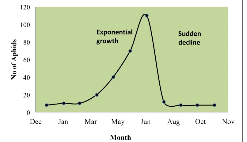
Density-independent birth rates and death rates do NOT depend on population size; these factors are independent of, or not influenced by, population density. Many factors influence population size regardless of the population density, including weather extremes, natural disasters (earthquakes, hurricanes, tornadoes, tsunamis, etc.), pollution and other physical/abiotic factors. For example, an individual deer may be killed in a forest fire regardless of how many deer happen to be in the forest. The forest fire is not responding to deer population size. As the weather grows cooler in the winter, many insects die from the cold. The change in weather does not depend on whether there is a population size of 100 mosquitoes or 100,000 mosquitoes, most mosquitoes will die from the cold regardless of the population size and the weather will change irrespective of mosquito population density. Looking at the growth curve of such a population would show something like an exponential growth followed by a rapid decline rather than levelling off (Figure 2.6).
20 40 60 80 100 120
No of
Aphids
Exponential
growth Sudden decline
0
Dec Jan Mar May Jun Aug Oct Nov
[image:31.612.86.489.56.289.2]Month
Figure 2.6: Weather change acting as a density-independent factor limiting aphid population growth.
This insect undergoes exponential growth in the early spring and then rapidly die off when the weather turns hot and dry in the summer
In real-life situations, density-dependent and independent factors interact. For example, a devastating earthquake occurred in Haiti in 2010. This earthquake was a natural geologic event that caused a high human death toll from this density-independent event. Then there were high densities of people in refugee camps and the high density caused disease to spread quickly, representing a density-dependent death rate.
Q: Can you think of other density-dependent (biological) and density-independent (abiotic)
population limiting factors?
2.4 Life Tables and Survivorship
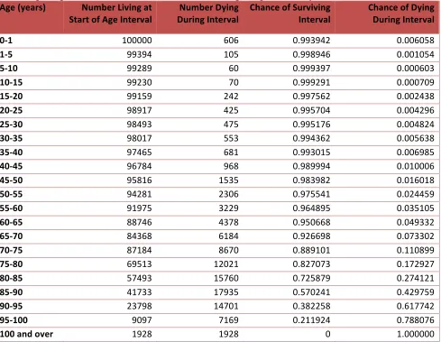
Population ecologists use life tables to study species and identify the most vulnerable stages of organisms’ lives to develop effective measures for maintaining viable populations. Life tables, like
Table 2.1, track survivorship, the chance of an individual in a given population surviving to various
ages. Life tables were invented by the insurance industry to predict how long, on average, a person will live. Biologists use a life table as a quick window into the lives of the individuals of a population, showing how long they are likely to live, when they’ll reproduce, and how many offspring they’ll produce. Life tables are used to construct survivorship curves, which are graphs showing the proportion of individuals of a particular age that are now alive in a population. Survivorship (chance of surviving to a particular age) is plotted on the y-axis as a function of age or time on the x-axis. However, if the percent of maximum lifespan is used on the x-axis instead of actual ages, it is possible to compare survivorship curves for different types of organisms (Figure 2.7). All survivorship curves start along the y-axis intercept with all of the individuals in the population (or 100% of the individuals
[image:32.612.59.548.150.529.2]
surviving). As the population ages, individuals die and the curves goes down. A survivorship curve never goes up.
Table 2.1: Life Table for the U.S. population in 2011 showing the number who are expected to be
alive at the beginning of each age interval based on the death rates in 2011. For example, 95,816 people out of 100,000 are expected to live to age 50 (0.983 chance of survival). The chance of surviving to age 60 is 0.964 but the chance of surviving to age 90 is only 0.570.
Age (years) Number Living at Number Dying Chance of Surviving Chance of Dying Start of Age Interval During Interval Interval During Interval
0-1 100000 606 0.993942 0.006058
1-5 99394 105 0.998946 0.001054
5-10 99289 60 0.999397 0.000603
10-15 99230 70 0.999291 0.000709
15-20 99159 242 0.997562 0.002438
20-25 98917 425 0.995704 0.004296
25-30 98493 475 0.995176 0.004824
30-35 98017 553 0.994362 0.005638
35-40 97465 681 0.993015 0.006985
40-45 96784 968 0.989994 0.010006
45-50 95816 1535 0.983982 0.016018
50-55 94281 2306 0.975541 0.024459
55-60 91975 3229 0.964895 0.035105
60-65 88746 4378 0.950668 0.049332
65-70 84368 6184 0.926698 0.073302
70-75 87184 8670 0.889101 0.110899
75-80 69513 12021 0.827073 0.172927
80-85 57493 15760 0.725879 0.274121
85-90 41733 17935 0.570241 0.429759
90-95 23798 14701 0.382258 0.617742
95-100 9097 7169 0.211924 0.788076
100 and over 1928 1928 0 1.000000
SOURCE: CDC/NCHS, National Vital Statistics System.
Survivorship curves reveal a huge amount of information about a population, such as whether most offspring die shortly after birth or whether most survive to adulthood and likely to live long lives. They generally fall into one of three typical shapes, Types I, II and III (Figure 2.7a). Organisms that exhibit Type I survivorship curves have the highest probability of surviving every age interval until old age, then the risk of dying increases dramatically. Humans are an example of a species with a Type I survivorship curve. Others include the giant tortoise and most large mammals such as elephants. These organisms have few natural predators and are, therefore, likely to live long lives. They tend to produce only a few offspring at a time and invest significant time and effort in each offspring, which increases survival.
In the Type III survivorship curve most of the deaths occur in the youngest age groups. Juvenile survivorship is very low and many individuals die young but individuals lucky enough to survive the first few age intervals are likely to live a much longer time. Most plants species, insect
species, frogs as well as marine species such as oysters and fishes have a Type III survivorship curve. A female frog may lay hundreds of eggs in a pond and these eggs produce hundreds of tadpoles. However, predators eat many of the young tadpoles and competition for food also means that many tadpoles don’t survive. But the few tadpoles that do survive and metamorphose into adults then live for a relatively long time (for a frog). The mackerel fish, a female is capable of producing a million eggs and on average only about 2 survive to adulthood. Organisms with this type of survivorship curve tend to produce very large numbers of offspring because most will not survive. They also tend not to provide much parental care, if any.
Type II survivorship is intermediate between the others and suggests that such species have an
even chance of dying at any age. Many birds, small mammals such as squirrels, and small reptiles, like lizards, have a Type II survivorship curve. The straight line indicates that the proportion alive in each age interval drops at a steady, regular pace. The likelihood of dying in any age interval is the same.
In reality, most species don’t have survivorship curves that are definitively type I, II, or III. They may be anywhere in between. These three, though, represent the extremes and help us make predictions about reproductive rates and parental investment without extensive observations of individual behavior. For example, humans in less industrialized countries tend to have higher
mortality rates in all age intervals, particularly in the earliest intervals when compared to individuals in industrialized countries. Looking at the population of the United States in 1900 (Figure 2.7b), you can see that mortality was much higher in the earliest intervals and throughout, the population seemed to exhibit a type II survivorship curve, similar to what might be seen in less industrialized countries or amongst the poorest populations.
a b
Figure 2.7: (a) Survivorship curves show the distribution of individuals in a population according to age. Humans and most large mammals have a Type I survivorship curve because most death occurs in the older years. Birds have a Type II survivorship curve, as death at any age is equally probable. Trees have a Type III survivorship curve because very few survive the younger years, but after a certain age, individuals are much more likely to survive. (b) Survivoship curves for the US population for 1900, 1950, 2000, 2050, 2100
SOURCE: www.ssa.gov.
******************************************************************************
This material has been modified from the OpenStax Biology textbook.
POPULATION ECOLOGY PRACTICE PROBLEMS
1. If a population is experiencing exponential growth, what happens to N, r and G over time (increase, decrease or stay the same)?
2. At the beginning of the year, there are 7650 individuals in a population of beavers whose per capita rate of increase for the year is 0.18. What is its population growth rate at the end of the year?
3. A zebrafish population of 1000 individuals lives in an ecosystem that can support a maximum of 2000 zebrafish. The per capita rate of increase for the population is 0.01 for the year. What is the population growth rate?
4. In a scenario where: r = 0.25; K = 18,000;
a. What is G when i) N = 4,500; ii) N = 9,000; and iii) N = 13,500? b. Which N level results in the highest population growth rate and why?
5. A chipmunk population is experiencing exponential growth with a population growth rate of 265 individuals/year, and a per capita rate of increase of 0.15. How many chipmunks are currently in this population?
6. Scientists discovered a new species of frog and were able to estimate its population at 755 individuals. At the end of the year, 105 frogs were added to this population. Assuming the population is undergoing exponential growth, what is the per capita rate of increase?
Test your skills (extra challenge)
7. At the beginning of the year, a wildlife area that is 1,000,000 ha in size has a population of 90 Brown bears with a per capita growth rate of 0.02. It’s estimated that brown bears need a territory of about 10 km2 per individual (note: 1 km2 = 100 ha). Use this information to answer the
following questions.
a. What is the density of brown bears in this wildlife preserve currently? b. What is the carrying capacity of the preserve?
c. What is the population growth rate for this year?
8. A wildlife ranch currently has a population of polar bears whose death rate is 0.05 and birth rate is 0.12 per year. This particular ranch is isolated from other suitable habitats so there’s no
immigration into or emigration from this population. This population is experiencing logistic growth and currently has 550 bears. If the population growth rate for the year was 36 bears, what is the carrying capacity of the preserve?
Return to Table of Contents
Chapter 3: Human
D
emography
By the end of this chapter, you will be able to:
• State the current size of the human population. • Interpret age-structure diagrams.
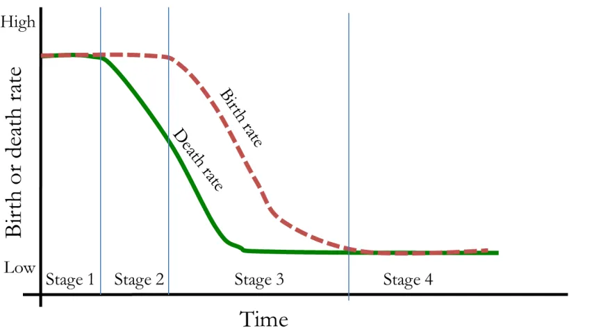
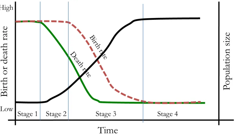
• Explain what the demographic transition model represents and describe the societal changes that cause the demographic transition.
• Describe what happens to birth rates, death rates, population growth rate, and population size as a country moves through the stages of the demographic transition model.
• Give examples of countries in the different stages of the demographic transition models and match age-structure diagrams with the stages of the demographic transition model.
• Define life expectancy and explain how it changes as a country moves through the demographic transition model.
• Define fertility and explain how it changes as a country moves through the demographic transition model.
Chapter outline
1. The human population 2. Demography
3. Age structure diagrams
4. The demographic transition model 5. Life expectancy
6. Fertility
3.1 The human population.
The human population is growing rapidly. For most of human history, there were fewer than 1 billion people on the planet. During the time of the agricultural revolution, 10,000 B.C., there were only 5-10 million people on Earth - which is basically the population of New York City t