CSG based automatic mesh generation using multiple element types

Rochester Institute of Technology

RIT Scholar Works

Theses

Thesis/Dissertation Collections

8-1-1993

CSG based automatic mesh generation using

multiple element types

Richard H. Hall

Follow this and additional works at:

http://scholarworks.rit.edu/theses

This Thesis is brought to you for free and open access by the Thesis/Dissertation Collections at RIT Scholar Works. It has been accepted for inclusion

in Theses by an authorized administrator of RIT Scholar Works. For more information, please contact

[email protected]

.

Recommended Citation

Approved by:

CSG BASED AUTOMATIC MESH GENERATION

USING MULTIPLE..ELEMENT TYPES

by

Richard H. Hall

A Thesis Submitted

In

Partial Fulfillment

of the

Requirements for the Degree of

MASTER OF SCIENCE

In

Mechanical Engineering.

Prof.~

_

Dr.

Richard Budynas (Thesis Advisor)

Prof.

_

Dr.

Joseph Torok

Prof.

_

Mr.

Guy Johnson

Prof.

_

Dr.

Charles Haines (Department Head)

Department of Mechanical Engineering

College of Engineering

Title of Thesis -- "CSG Based Automatic Mesh Generation using Multiple Element Types"

I, Richard H. Hall, hereby grant pennission to the Wallace Memorial Library of R.I.T. to

reproduce my thesis in whole or

in

part. Any reproduction will not

be

for commercial use or

profit.

Date: 10/21/93

Abstract

The

objective ofthis thesisproject

is

toexplore aunique approachtowardautomatic mesh

generation

for finite

element analysis.

Current

mesh generationalgorithms are

only

applicable to a singletype of

domain.

Countless

meshgeneratorsexist

for meshing 2D

regions with triangles and

quadrilaterals, and mesh generators also existwhich can mesh

3D

regionswith tetrahedraand

other elementtypes.

However,

not all structures are

strictly

"2D"

or

"3D",

and not all structures

are

best

modeledwitha singletype of element.

An

experienced

finite

element analyst

typically

uses

many

typesofelements when

modeling

a real problem.

This

thesisaddresses this approach to

meshing in

anautomatic manner.

However,

atvarious stages, the user

has

the

ability

tochange

thecourse ofthemodeler.

In

this thesis project,aprogram

for

automatic mesh generation

has been developed

on a

constructive solid

geometry

(CSG)

foundation. This

program waswritten

in

object-oriented

Pascal,

and consistsof well over

25,000

lines

of code.

The

CSG

system used was

developed

with

PADL-2

asthe guide, and allowscomplex geometriesto

be

modeled as combinations of

blocks

andcylinders.

This

solidmodel

is

then

broken

into

ID,

2D

and

3D

regions, or

"segments",

using

CSG-Tree

segmentation

logic. Each

segmentcanthen

be

meshed

using

an appropriate mesh

generationtechnique.

Thus,

a singlemodelcan

be

meshedwithmultiple element

types, just

as an

Acknowledgments

This

thesis

has been

a

long

time

in

themaking, which

has

given

many

people a chance to

contribute.

I

would

like

to thankeveryone who made the

writing

ofthis thesispossible:

Dr. Richard

Budynas,

who

has been envisioning

a computer program toperform

automatic mesh generator

using

multiple elementtypes

for

a

long,

long

time. I'm

thankful to

Dr.

Budynas

for

having

confidence

in

_me,

believing

that

I

would

be

able tomake

his dream

areality,

and

for

his

continued support and encouragement.

I only

hope

thatwhat

I have

produced

does

justice

to what

he had in

mind.

Committee

members

Dr. Joseph Torok

and

Mr.

Guy

Johnson,

who

deserve extraordinary

credit

just for reading

such a

fat,

boring

book. Dr. TOrok's

knowledge

of

finite

element

theory

and

Guy

Johnson's knowledge

of geometric

modeling

and

programming

were

instrumental in

writing

the

finished

version ofthisthesis, and theircontributions are

greatly

appreciated.

Mr.

Steve

Kurtz,

who's course

"Computer Graphics is

Design" taughtme object-oriented

Pascal

and, more

importantly,

enthusiasm

for

elegant programming.

Without

having

picked

up

thisenthusiasm

from

Steve,

writing 25,000

lines

of code would not

have been

possible.

Dr.

Charles

Haines,

department

head

and academic advisor.

As

a

BS/MS

student,

I'd like

to thank

Dr. Haines

for

making

me

feel

like

therewas someone

looking

out

for

me.

The Gleason

Society,

for

the

honor

and

financial

support of

being

selected asthe

1991/92

Gleason

Graduate

Scholar.

Thanks

to

Megan,

who

has been

an

important

part of

my

life

and can never

be anything

less.

And

finally,

I

would

like

toexpress

my

appreciation and gratitude

for my

parents,

Harley

and

Sandy,

for

their

never-ending

patience and support.

This

thesisand

every

success

in my life is

Table

of

Contents

Abstract

iii

Acknowledgments

iv

List

of

Figures

viii

List

of

Symbols

xiii

1. Introduction

1

1.1. The Finite Element Method in Mechanical

Engineering

1

1.2.

History

ofthe

Finite Element Method

2

1.3. Finite Element

Theory

4

1.4. Types

and

Uses

of

Finite Elements

7

1.4.1. One-Dimensional Second-Order Equations

7

1.4.2. One-Dimensional Fourth-Order Equations

12

1.4.3. Two-Dimensional Scalar Valued Second-Order Equations

16

1.4.4. Two-Dimensional

Multi-

Variable Equations

21

1.4.5.

Three-Dimensional

Equations

22

1.5.

Modeling

using Multiple Element Types

23

1.6. Thesis Objective

24

2. Automatic Mesh Generation

Review

of

Related

Literature

25

2.1.

History

of

Mesh

Generation

25

2.2. Automatic

Meshing

of

1-D Regions

26

2.3. Automatic

Meshing

of

2-D Regions

27

2.3.1.

Volume

Triangulization

Methods

27

2.3.2. Element

Extraction

Methods

32

2.3.3. Recursive Spatial Decomposition Methods

35

2.4. Automatic

Meshing

of

3-D Regions

37

2.4.1. Volume

Triangulization

Methods

37

2.4.2. Element Extraction Methods

39

2.4.3. Recursive Spatial Decomposition Methods

40

2.5. Expert Systems for Automatic Mesh Generation

41

3. Geometric

Modeling

44

3.1.

Modeling

Techniques

44

3.1.1.

Sweep

Representations

45

3.1.2. Cell

Decompositions

45

3.1.3.

Boundary

Representation

46

3.1.4. Constructive Solid

Geometry

47

3.2.

Boundary

Evaluation

48

4. Expert S

ystems

53

4.1. Expert

System Structure

53

4.2.

Expert

System

Development

55

5.

CSG

Based

Automatic

Mesh

Generation

using Multiple Element Types

58

5.1.

"CSGMesh"

Computer

Program

59

5.1.1. Program Overview

60

5.1.1.1. Input File

60

5.1.1.2.

CSG

Tree

66

5.1.1.3. Segments

70

5.1.1.4. Options

73

5.1.1.5. Meshes

76

5.1.1.6. Output File

83

5.1.2.

Solid Representation

85

5.1.2.1. Solids

86

5.1.2.1.1. Blocks

88

5.1.2.1.2.

Cylinders

88

5.1.2.1.3. Other Primitives

89

5.1.2.1.4. Unions

89

5.1.2.1.5. Differences

90

5.1.2.1.6. Intersections

90

5.1.2.2.

Boundary

Representation

90

5.1.2.2.1. Surfaces

92

5.1.2.2.2.

Edges

93

5.1.2.3.

Boundary

Evaluation

94

5.1.3.

Segments

98

5.1.3.1. BeamSegments

98

5.1.3.2. PlateSegments

99

5.1.3.3.

CylinderPlateSegments

99

5.1.3.4. BrickSegments

99

5.1.3.5. CSG Segmentation Logic

100

5.1.3.5.1. Blocks

103

5.1.3.5.2.

Cylinders

103

5.1.3.5.3.

Unions

103

5.1.3.5.4.

Differences

104

5.1.3.5.5. Intersections

104

5.1.3.5.6. Special

Cases

104

5.1.3.5.7.

Using

Surfaces

tomake

Segments

106

5.1.3.5.8.

Combining

Segments

106

5.

1

.4.

Segment

Meshing

Techniques

108

5.1.4.1. Types

of

Meshes

108

5.1.4.2.

Meshing

Beam

Segments

109

5.1.4.3.

Meshing

Plate

Segments

109

5.1.4.4.

Meshing

CylinderPlate Segments

111

5.1.4.5.

Meshing

Brick

Segments

112

5.1.4.6.

Editing

Meshes

113

5.2. Future Extensions

to "CSGMesh"

5.2.1. Further Primitive

Types

5.2.2.

Implementing

Mesh

Generators

5.2.3.

Other

possible additionsto "CSGMesh"

Results: Examples

of

Geometries

Meshed

using

"CSGMesh"

6.1. Plate

with

Holes

6.1.1. Plate using Plate

Segment

(2D

Mesh)

6.1.2. Plate using Brick

Segment

(3D

Mesh)

6.2.

I-Beam

6.2.1.

I-Beam using Beam

Segment

6.2.2. I-Beam using Plate

Segment

6.2.3. I-Beam using Multiple Plate

Segments

6.2.4. I-Beam using Brick

Segments

6.3.

Pipe

6.3.1.

Pipe using Beam Segment

6.3.2. Pipe using Plate

Segment

6.3.3. Pipe using

CylinderPlate Segment

6.3.4. Pipe using Brick

Segment

6.4. Pipe

with

Holes

6.5. Bracket

114

115

120

122

127

127

129

130

132

133

134

135

136

137

138

139

140

141

142

145

7. Discussion/Conclusion

8. References

150

151

9. Appendices:

Appendix A.

Appendix

B.

Appendix

C.

Appendix

D.

Appendix

E.

Appendix F.

Appendix

G.

PADL-2

Source Files

PADL-2 Point

Sets:

Primitives, Halfspaces,

and

Edges

CSGMesh

Object

Hierarchy

CSGMesh

Object Reference

CSGMesh Input

(.CSG)

File

Syntax Diagrams

Algor

Supersap

Output File

ANSYS

version

5.0 Output File

Appendix

H.

NASTRAN

Output File

List

of

Figures

Figure

Page

Chapter 1:

Figure 1.1

Division

of circle

into

triangles

2

Figure 1.2

Generic Domain

Q

4

Figure 1.3

Strong

and

Weak

Statements

5

Figure 1.4

One-Dimensional Domain for

Second-Order Equations

7

Figure 1.5

Typical

One-Dimensional,

Second-Order Element

8

Figure 1.6

Interpolation Functions for ID Two-Node Linear Element

1 1

Figure 1.7

One Dimensional Domain for Fourth-Order

Equations

12

Figure 1.8

Interpolation Functions for ID Two-Node

Quadratic

Element

15

Figure 1.9

Two-Dimensional Domain

16

Figure 1.10

Two-Dimensional

Elements

1

8

Figure 1.11

Interpolation Functions for 2D Three-Node Linear Triangle

Elements

19

Figure 1.12

Four-Node Rectangular Element Local Coordinate System

19

Figure

1.13

Interpolation

Functions for 2D

Four-

Node Linear Quadrilateral Elements

20

Figure 1.14

Three-Dimensional

Elements

22

Figure 1.15

Mesh using Different Element Types

23

Chapter

2:

Figure

2. 1

Convex Hull

of a

Set

of

Points

28

Figure 2.2

Starting

Mesh

for

Delaunay

Triangulation

29

Figure 2.3

Node Insertion in

Delaunay

Triangulation

30

Figure 2.4

Delaunay

Triangulation

ofthe

Convex Hull

of a

Set

of

Points

3 1

Figure

2.6

Various

Stages

ofa

Paving

Algorithm

with

Fronts

by

Inflation

33

Figure 2.7

Various Stages

ofa

Paving

Algorithm

using

Quadrilaterals

34

Figure 2.8

Various

Stages

of a

Quadtree Algorithm

35

Figure 2.9

Mesh

Generated

by

Quadtree

Algorithm

36

Figure

2. 10

Mesh

Generated

by

3D

Delaunay

Triangulation

38

Figure

2.11

Mesh

Generated

by Plastering

Algorithm

39

Figure 2.12

Mesh

Generated

by

Octree

Algorithm

40

Chapter

3:

Figure 3. 1

Sweep

Representation

45

Figure 3.2

Boundary

Representation

(B-Rep)

46

Figure 3.3

Constructive Solid

Geometry

(CSG)

Representation

47

Figure 3.4

Polygonal Representation

of

CSG Primitives

49

Figure

3.5

Polygonal Representation

of

CSG Solid

49

Figure

3.6

PADL-2 Block

51

Figure

3.7

PADL-2

Cylinder

51

Figure

3.8

PADL-2 Wedge

51

Figure

3.9

PADL-2

Cone

51

Figure

3.10

PADL-2 Sphere

51

Figure

3.11

PADL-2

Torus

51

Chapter 4:

Figure

4.

1

Expert System Structure

54

Chapter

5:

Figure 5. 1

CSGMesh

File Menu

6

1

Figure 5.2

Block in

standard position

62

Figure 5.3

Cylinder

in

standard position

64

Figure 5.4

Operations

on

Block

and

Cylinder

65

Figure 5.5

Typical

CSG Input

File

65

Figure 5.6

CSGMesh

CSG-Tree

Menu

66

Figure 5.7

CSG Tree

67

Figure 5.8

CSGMesh

CSG Tree

and

SolidList

67

Figure 5.9

Sketch

of

CSG Tree Primitives

69

Figure 5.10

CSGMesh Segments

Menu

70

Figure 5.11

Drawing

of

Segment

(Solid)

7 1

Figure 5.12

Drawing

of

Segment

(Representation)

72

Figure 5.13

CSGMesh Options Menu

73

Figure 5.14

Material Definition

Dialog

Box

74

Figure 5.15

CSGMesh Mesh Menu

76

Figure 5.16

Mesh

of

Segment

(Plate)

78

Figure 5.17

Mesh

of

Segment

(Brick)

78

Figure

5.18

Fine Mesh

of

Segment

79

Figure

5.19

Course

Mesh

of

Segment

80

Figure 5.20

Course Mesh

of

Segment

with

Node Added

80

Figure 5.21

Two

Adjoining

Plate

Segments

81

Figure 5.22

Two

Adjoining

Plate Segments Merged

82

Figure 5.23

Two

Adjoining

Plate Segments Merged

and

Connected

82

Figure 5.24

Mesh Loaded into Algor

Supersap

83

Figure 5.25

Mesh Loaded

into ANSYS

version

5.0

84

[image:12.563.51.481.50.701.2]

Figure 5.27

SolidList

and

CSGTree

Data Structures

87

Figure

5.28

Solid

Object

Hierarchy

88

Figure

5.29

Operation Data

Structure

90

Figure 5.30

Boundary

Representation Data

Structure

91

Figure 5.31

Surface Outside

Sense

92

Figure 5.32

Example

of

Boundary

Evaluation

Sequence

95

Figure

5.33

Table (Example

of

CSG Tree

Segmentation)

100

Figure 5.34

CSG Tree

of

Table

100

Figure 5.35

HollowBlock Special Case

105

Figure

5.36

Re-

Definition

_of

HollowBlock

105

Figure 5.37

Node Generation in Plate

Segments

1 10

Figure 5.38

Node Generation in CylinderPlate

Segments

111

Figure 5.39

Meshing

of

Brick

Segments

1 13

Chapter

6:

Figure 6.1

Plate

with

Holes

-

Primitives

128

Figure 6.2

Plate

with

Holes

-

Solid

_after

Boundary

Evaluation

128

Figure

6.3

Plate

with

Holes

as

Plate Segment

129

Figure 6.4

Mesh

of

Plate

with

Holes

as

Plate Segment

130

Figure

6.5

Plate

with

Holes

as

Brick Segment

131

Figure

6.6

Mesh

of

Plate

with

Holes

as

Brick

Segment

1

3

1

Figure

6.7

I-Beam

-

Primitives

132

Figure

6.8

I-Beam

as

Beam Segment

133

Figure

6.9

Mesh

of

I-Beam

as

Beam Segment

133

Figure

6.10

I-Beam

as

Plate Segment

134

Figure 6.11

Mesh

of

I-Beam

as

Plate Segment

1

34

Figure 6.12

I-Beam

as

Multiple Plate Segments

135

Figure

6.13

Mesh

of

I-Beam

as

Multiple

Plate Segments

1

35

Figure 6.14

I-Beam

as

Brick Segment

136

Figure

6.15

Mesh

of

I-Beam

as

Brick

Segment

136

Figure

6.16

Pipe

-Primitives

137

Figure

6.17

Pipe

as

Beam

Segment

138

Figure 6.18

Mesh

of

Pipe

as

Beam

Segment

1

3 8

Figure 6.19

Pipe

as

Plate

Segment

139

Figure 6.20

Mesh

of

Pipe

as

Plate

Segment

139

Figure 6.21

Pipe

as

CylinderPlate Segment

140

Figure 6.22

Mesh

of

Pipe

as

CylinderPlate

Segment

140

Figure 6.23

Pipe

as

Brick Segment

141

Figure 6.24

Mesh

of

Pipe

as

Brick

Segment

141

Figure 6.25

Pipe

with

Holes

-

Primitives

142

Figure

6.26

Pipe

with

Holes

Solid

after

Boundary

Evaluation

143

Figure

6.27

Pipe

with

Holes

-

Plate

Segment

Representation

143

Figure

6.28

Mesh

of

Pipe

with

Holes

144

Figure 6.29

Mesh

of

Pipe

with

Holes

144

Figure

6.30

Bracket

~

Primitives

145

Figure

6.3

1

Bracket

-

Solid

after

Boundary

Evaluation

146

Figure 6.32

Bracket

-

Plate Segment Representation

147

Figure

6.33

Bracket

-

Plate Segment Representation (End

View)

147

Figure 6.34

Bracket

-

Mesh

148

Figure

6.35

Bracket

~

Mesh

(End

View)

148

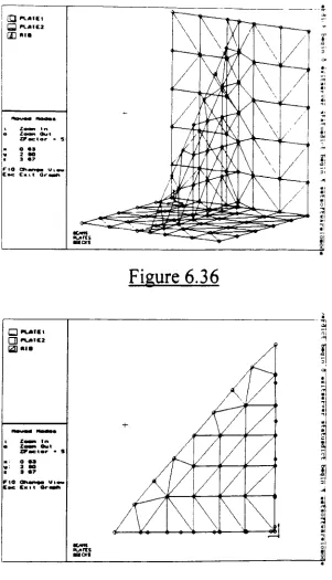
Figure

6.36

Bracket

-

Mesh

after

Merging

and

Connecting

149

Figure

6.37

Bracket

--

Mesh

[image:13.563.55.478.45.646.2]

List

of

Symbols

Bold

letters

Vector

or

Matrix

a unknown parameter

in

approximation

function

A

Differential

operator

B(v,u)

Bilinear

functional

ofuand v

BLO

Block

primitive

CON

Cone

primitive

CSG

Constructive Solid

Geometry

CYL

Cylinder

primitive

DIP

Difference

operation

DOF

Degree

of

Freedom

e

Typical

Element

E

Modulus

of

Elasticity

(Young's

Modulus)

EBC

Essential

Boundary

Condition

/

forcing

function

F(e)

Force Vector

for

_{element e}

FEA

Finite Element Analysis

FEM

Finite Element Method

G

Shear

Modulus

INT

Intersection

operation

Ixx

Moment

of

Inertia

about x-axis

Ixy

Product

of

Inertia

Iyy

Moment

of

Inertia

about y-axis

J

Polar Moment

of

Inertia

K(e)

Stiffness

Matrix

for

elemente

l(y)

Linear

functional

ofv

M[X,

S]

Classify

X

against

S

MCR

Membership

Classification Result

NBC

Natural

Boundary

Condition

PADL

Part

and

Assembly

Description (or

Definition)

Language

RSD

Recursive Spatial Decomposition

SPH

Sphere

primitive

TOR

Torus

primitive

u unknown

function

UN

Union

operation

WED

Wedge

primitive

v test

function

1. Introduction

1.1. The Finite

Element Method

in Mechanical

Engineering

In

today's

highly

competitive_world, products must

be

designed

very

carefully.

Modern

engineers must ensurethat their

designs

will

be

functional,

last

when subjectto

hard

use and extreme

conditions,

be

attractive and

pleasing

_{to the user,} achieve

high

standards

in

termsof

safety,

and will

satisfy

a multitude of other consumer

demands.

In

additiontoall ofthese

requirements,

designs

must

be

cost-effective as well.

Fortunately,

a modern

design

engineer

is

not requiredtoproduce a prototype of

each of

his design

alternativesto submitto

testing

of allthe

necessary

criteria.

This surely

wouldnot

be

cost effective.

There

are severaltechniquesavailable

in

whichtheengineer

can represent

his design

mathematically

to testvarious parameters.

One

ofthemost

powerful, and

certainly

themost_popular,

is

the

Finite Element Method

(FEM).

In

the

Finite Element

Method,

a complex

geometry is broken down into

a

finite

numberof simple geometric_shapes, called

finite

elements.

The

material properties and

governing

relationships

(usually

a set of

differential equations)

areexpressed overthese

elementstoyield a system of equations.

These

equations can

be

solvedtogivethe

1.2.

History

ofthe

Finite

Element

Method

The

idea

of

representing

_{a given}

domain

_{with anumber ofsimple geometric shapes}

is

not new.

Ancient

_{mathematiciansestimatedthevalue of pi accurateto}

40

_places

by

representing

a circle with a

large

number oftriangles as shown

in figure

1

.

1

Typical

"element"

h

Ae=

4rbh

Figure

1.1

In

modern

times,

the

basic ideas

ofthe

finite

element method originated

in

the

aircraft

industry,

where wings and

fuselages

were represented as collections of

strings,

skins, and shear panels.

In

1941,

HrenikofT

presented the

"frame-work

_method,"[11

in

whichplane elastic regions were modeled

using

acollectionof

bars

and

beams. The

use

of piecewise continuous

functions dates

to

1943,

when

Courant

useda collection of

triangularelements andtheprinciple of minimum potential

energy

to

study

the

St. Venant

Torsion

problem.121

The formal

_{presentationofthe}

finite

_{element method}

is

attributedto

Turner, Clough, Martin,

and

Topp,

who

in

1956

derived

stiffness matrices

for

truss,

beam,

and otherelements,!31 _andto

Argyris

_and

Kelsey,

who wrotetheirpaper on

Energy

Theorems

and

Structural Analysis

in

1960.[4]

The

_term

"finite

element"

was

first

coined

In

the

early

1960's,

_{engineersused the}

finite

_{element methodto}

find

_approximate

solutionsto problems

in

stress

analysis,

fluid

flow,

heat

transfer,

and other areas.

The

first

book

on

finite

elements

by

Ziekiewicz

and

Chung

was published on 1967.[5]

In

the

late

1960's

and

early

1970's,

the

finite

element method was appliedtonon-linear problemsand

large deformations.

A

book

on non-linear continua

by

Oden

appeared

in 1972.

[6]

Mathematical

foundations

were

laid in

the

1970's,

including

element

development,

convergence

studies,

and other related studies.

Since its

inception,

the

literature

onthe

finite

element method

has

grown

exponentially,

and

today

thereare numerous

journals

whichare

devoted primarily

to the

theory

and application ofthe

finite

element method.

A

reviewofthe

historical

developments

andthe

basic

theory

ofthemethod can

be found

in

dozens

oftextbooksthat

1.3. Finite

Element

Theory

As

with

any

numerical

technique,

an

understanding

ofthe

underlying

principlesof the

FEM

is necessary in

ordertousethemethod effectively.

However,

it

would not

be

practicalto

include

athorough

discussion

ofthe

theory

ofthe

finite

element method

in

this

thesis.

Volumes

upon volumes

have been

written aboutthe

theory

and application ofthe

finite

elementmethod.

The

purpose ofthis thesis

is

toexplorethearea of automatic mesh

generation, and notto explain

fully

the

theory

and concepts ofthe

finite

element method.

Thus,

the subject of

finite

element

theory

will

be limited

to a

brief summary discussion.

The Finite Element Method

is

a piecewiseapplicationof avariationalmethod.

A

typicalproblem

involves

some

domain

Q,

defined

by

a

boundary

T,

overwhich some

mathematical relations

hold.

The

objectiveofthe analysis

is

to

determine

unknown

functions

which

satisfy

themathematical relations

(usually

differential equations)

overthe

domain. Figure 1.2

shows a generic

domain

Q.

overwhicha set of

differential

equations

describe

the

behavior.

Boundary J7

Applied

Force

Governing

Equation: Au

=

f

A

= _{differentialoperator} u = _unknown

function

f

=

forcing

function

Edge Fixed

In

ordertomake use ofthe

finite

elementmethod, the

governing

equations

describing

the

behavior

ofthe

domain

must

be

cast

in

"weak"

(or

variational)

form. The

differential

equation

Aw

=/is saidto

be in

the"strong"

form,

meaning

thatthe equation

represents an exact statementat

every

point

in

the

domain.

To

obtaintheweak

form,

test

functions

(represented

by

"v")

must

be

chosen which are

sufficiently differentiable

and

whichtakeonthevalue zero at

Essential

Boundary

Condition

(EBC)

locations.

Both

sides ofthe

strong form

are multiplied

by

the test

function

vandthen

integrated

overthe

domain,

yielding

j(Au-f)vdQ

=

0.

a

An analogy

which

helps

tomaketheconcepts of"strong" and "weak"

forms

more clear

is

that of some simple

function,

say

g(x).

The

statement

g(x)

=

₀

for 0

_{< x <}

L

is

a

strong

statement.

It

saysthatat

every

point

between

0

and

L,

thevalue of

g

is

identically

zero.

However,

thestatement

\g(x)dx

=

0

is

_{a muchweakerstatement.}

It

_allowsthe

value of

g

to

be

something

otherthanzero

between

0

and

L,

as

long

astheaverage value overthe

domain is

zero.

This forces

the

arbitrary

function

g(x)

toapproximate zero as

closely

as possible

between

0

and

L. This

is

shown

in figure

1.3.

*00

g(*)=

o

utmr,^_^^jt

strong statement

g

i ^ i

L

x

₀

gCO*0

L

g(x)dx =

₀

"weak"

statement

L

x

After

the

differential

equation

is

cast

in

weak

form,

thenext

step is

to

integrate

by

partstotransferthe

differentiation from

the

dependent

variableuto thetest

function

v.

This

servestoreducethe

differentiation

requirementon

u,

whichallows

lower-order

functions

to

be

usedtoapproximatethe

behavior

ofthesystem.

In

theprocess of

integrating by

parts,

boundary

termsare obtainedwhich

identify

thenature ofthe

boundary

conditions

in

thesolution.

By

setting

v=

₀

at

Essential

Boundary

Condition

(EBC) locations,

and

defining

secondary

variables at

Natural

Boundary

Condition

(NBC)

locations,

the

boundary

conditions

become imposed into

the

functional.

The

weak

form becomes

thusposed as:

find

u suchthat

B(w,v)

-/(v)

for

alltest

functions

vsuchthatv=

₀

at

EBC

locations,

where

B

is

bilinear functional representing

theweak

form

and

/ is

linear

functional

representing

the

boundary

terms.

This

processwill

be

shownmore

clearly

as

it is

usedto

develop

element equations

1.4. Types

and

Uses

of

Finite

Elements

The

finite

elementmethod

is

applicabletocountless problems posed on

many

domains.

Each

typeof problem and each

domain have

theirownunique set of equations.

In

thissection a

few

problemswill

be

consideredto

demonstrate

therequirements

for

casting

an equation

in

variational

form

over a

domain.

1.4.1.

One-Dimensional Second-Order

Equations

Consider

the problem of

finding

the

function

u whichsatisfiestheequation

d_

dx

'&'-applied overthe

domain

0

< x <

L,

andthe

boundary

conditions

w(0)

=

₀

and

a^\ =

P

, where a =

a(x),f=f[x)

and

P

are given

data

oftheproblem.

This

x=L

dx

equation arises

in

theaxial

deformation

of a

bar.

The

domain

Q=(0, L)

of_{the problem,} shown

in figure

1.4(a),

is divided into

a set of

line

elements, calledthe

finite

element_mesh, as shown

in

figure

1.4(b).

p

(a)

Physical

Problem

nodes

p

(b)

Finite

Element

Mesh

Since

the

governing

differential

equation

is

valid overthewhole

domain O

=

(0,L),

it is

valid overeachelementofthe

finite

element mesh.

In particular,

it is

validover

generic element e.

Following

theprocedure

described

in

section

1.3,

thevariational

formulation

ofthe

governing

differential

equation can

be

constructed over element e:

The

strong form is

given

by

\a

]-/=

0

overthe

domain

of element _e,

dx\ dx)

Qe

=

(*A,*B)

as shown

in

figure

1.5.

local

node

1

u(xA)-u[e)

(--)

-

tf>

O

local

node

2

u(xB)-u^

x=

xft

(--)

s PM

x=_x.

ilf

Figure 1.5

Multiplying

by

the test

function

vand

integrating

overthe

domain

yieldstheweak

form:

Jxa

d(

du

_{, ,}

a\-f

dx

dx

ctx=

₀

Integrating

by

partstotransferthe

differentiation

from

theunknown

function

uto

thetest

function

vgives:

)x\

dx dx

)

-a-du

Examining

the

boundary

term

in

theabove equation shows that thespecification of

u at x =

x and x =

xB

constitutetheessential

boundary

conditions,

andthespecification

1

~a~dY

I

at X =

*A

X =

Xb

constltutetnenatural

boundary

conditions

for

the

element.

Thus,

the

basic

unknowns atthe element nodes arethe

primary

variableu, which

is

the

degree

of

freedom

(DOF),

and the

secondary

variable

I

-a

)

To simplify

the

writing

ofthe

equations,

let

u(xa)

=u

du\

-a

.

dx)

,() - ,,,

eP,W

u(xb)

=U2

du

+a-dx

=P:(e) XB

Substituting

thisnotation

into

thevariational

form

gives

JxA\

dx dx

)

v(xa)-Piwv(xb)

=

0

fxsf a\

du

\ or

B(v,w)

-/(v)

=

₀

where

B(v,w)

is

the

bilinear

form

given

by B(v,u)

= a ax

Jx\

dx

dx)

and

/(v)

is

the

linear form

given

by

/(v)

=

[

vfdx+v(xa)Pim

+v(xs)P2(e) JXA

To

find

an approximate solutionto theabovevariationalproblem

using

the

Galerkin

method,

the

function

u

is

approximated overtheelement

by

n.(x)

=

2>(V,)(.t)

tt

(*

^^

AK

&,/dx

~ p,w

v^

PiW

v,(x,)

=

By

defining

the

local

stiffness

matrix,

K,

andthe

local force

_vector,

F,

as

follows,

K,"

=

B(V.,V,)=ra^*

JjM _{GDC &}

F,(c)

=

/(Vl)

=

J"v|/'/A

₊P*(e)

V'(xa)

+Pi(e)

v|/,(xrB)

theabove equation can

be

written

concisely in

matrix

form:

[K(c)]{a(e)}

=

{F(e)}.

All

that remains

is

to constructtheapproximation

functions,

\j/..

These

functions

are constructed

using

theconditions mentioned

in

section

1.3.

Namely,

theselected

functions

must

be sufficiently differentiable

and

satisfy

the essential

boundary

conditions of

the element.

They

must also

be

linearly

independent

and complete.

Three

ofthese

conditions are met

if

wechoose a

linear

approximation ofthe

form

ue(x)

=

cl

+ c2x.

In

orderto

satisfy

the

remaining

requirement, we require

ue

to

satisfy

the

EBC

ofthe

element.

Thus,

ci+ cixa =

u(xa)

=m(e)

c\+cixb

-u(xb)

= U2(e)

Solving

for

ct

and

c2

in

terms of

u^

and 2(e)_yields

UXWXB-U.WXA

2W-I/1W

C\ = _Cl

By

substituting

and

collecting coefficients,

it

can

be

shownthat

ue(x)

=

^

Ui{e)\\i,{e i=\

where \j/i(e) =

xb-x

VJ/2W =

X-Xa

, and x. < x <xE.

This

expression satisfiesthe

XB-Xa

Xb-Xa

essential

boundary

conditions of_{the element,} andthe approximation

functions

(v|/()

are

continuous and

linearly

independent

overtheelement.

These

interpolation

functions

for

the two-node

linear

element are shown

in figure

1.6.

Using

these

interpolation functions

to approximatethe

dependent

variable, the

following

matrix equationsareobtained:

M=r

1

-1

-1

1

[F(c)}

=

h

2

ll +

where

he

is

the

length

oftheelement

(xB

- _xA).

All

that_remains

is

toassemblethe

equations

derived for

each element

into

theglobal

finite

element

formulation.

This

process

is

straightforwardand

is

similar

for

all element

types,

so

it

will not

be

discussed

here.

1.4.2.

One-Dimensional Fourth-Order Equations

Consider

theproblem of

finding

the

function

uwhich satisfiestheequation

dx2\

dx2 J

applied overthe

domain

0

< x <

L,

where

b

=

b(x)

and/=

fix)

arethegiven

data

ofthe problem.

This

case arises

in

the

bending

of

beams.

As in

the second-order_{case, the}

domain is

discretized

into

subintervals, as shown

in figure

1.7.

nodes

M0

(a)

Physical Problem

(b)

Finite Element Mesh

Figure

1.7

The

variational

form

over atypicalelement e

is

given

by

J-v

JXA dx2

j

Integrating

twice

by

partsto transfer

half

ofthe

differentiation

from

wto vyields

r*B[

d2v

d2w

U

+vf

dx

+

v-dx

d2w

'dx2

dv

.

d2w

b

dx

dx2

dw

Inspection

ofthe

boundary

terms

indicates

that thespecification ofwand atx =

x.

dx

and x =

xB

constitutethe

EBC,

andthespecification of

d(,d2w^

dx

dx2

. Ld2w

and

b

-atx=x,

dx2 A

andx =

xB

constitutethe

NBC for

theelement.

Thus,

the

basic

unknownsattheelement

nodesarethe

primary

variables,which

for

notational conveniencewill

be

writtenas

,00_

wv ' =

w(xa)

so ^_<^_

dx

e.w = W2W =W(XB)

dx

andthe

secondary

variables, which will

be

writtenas

*

dx

{

dx2)

Q2M=bd a

2w

be2 X=XA () _ Q.w

-1

d

_w >

dx

Q*w=b

d2w

dx2

dx2

In

thecase ofthe

bending

of

beams,

the

primary

variables,wand

0,

represent

displacement

and_rotation, whicharethe

DOF

ofthe element, whilethe

secondary

variables,

Ql3

and

Q24,

representshear

forces

and

bending

moments.

Substituting

this

,

d2v

d2w

B(v'w>

=

Lb^^dx

l(v)

= _-f'vfdx+v(xA)Qi(e) JXA Q2Ce)-v(xs)Q3w +

'dv

^dx Q4(e)

The

variational

form

requiresthatthe

interpolation

functions

be

continuous with

continuous

derivatives

up

toorder

3

(so

that

Qt

and

Q3

arenonzero), and that

they

allow

theapproximation

for

wto

satisfy

the

EBC.

Since

thereareatotalof

four

conditions

in

an

element, a

four

parameterpolynomial

is

selected

for

wg:

wg(x)

=

ct

+ c^x +

c3x2

+ c^x3.

Forcing

the constraints

(EBCs),

wegetthesystem ofequations

1

Xa

Xa2

0

-1 -2xa

1

XB

XB1

0

-1 -2xb -3x XA1

'

Cl W\

3XA2

C2

01

i _r=

i > XSJ

C3 W2

3xs2_

C4

02

Solving

for

thec/s

in

termsof

wv

wv

0p

and

02,

and

substituting

theresults

back

into

wg

givesthe

interpolation functions:

Y|/lW=l-3,oo _i_il x XA i ₊₂ XB-XA X-Xa

\

xb-xaJ yxB-XA 2 H/3W =

3

XB-XA

X-Xa

\

J

X-XA

V|/400 =

-(x-x^)

x-x^ ^XB-X/f,

.2

X-Xa

These interpolation

functions

are shown

in figure

1.8.

Figure 1.8

Using

these

interpolation

functions,

the

following

element matrices result:

Kh

6

-3h -6 -3h

-3h 2h2

3/;

h2

-6

3h

6

3/j

-3h h2

3h

2h2

l*W]-Z

12

[6]

\QA

-h

6

+<

h

[Q*\

wheretheelement

displacement

vector

is

given

by

[u(e)

}

=

MM

01

M>2

02

1.4.3. Two-Dimensional

Scalar Valued

Second-Order Equations

Consider

theproblem of

finding

theequation uwhichsatisfiesthesecond-order

partial

differential

equation

(PDE)

5

(

bu

bu\

b

f

bu

bus

an van a2i 1-022

bxy

Sx

by)

by\

5x

by

+aoou-f=0

applied oversome

2-dimensional

region

Q,

as shown

in figure

1.9,

where a =

a

(x)

and/

=fix)

arethegiven

data

oftheproblem.

This

equation arises

in

2-dimensional

heat

transfer

in

an

isotropic

medium.

Boundary f

Finite Element

Mesh

Figure

1.9

The

variational

form is

given

by

J*

(

bx

bu

5a|

5

an +ai2

\-bx

by

J

by

(

bu

bu]

,

#21 +022

\

+aoou-t

bx

by)

dxdy

=

0.

Integration

by

parts

(with

some

help

from

the

divergence

theorem)

yields:

a'"L

Sv(

Su Su

8v[

5o 8m

f

Su Su

(

Su SuY

an₊

ai2 h 021 hau

8y^

8jc

Syj

+ aoovu -vf

dxdy- _iv

J

r<"

nx\ an \-an

{

Sx

Syj

+

"{a2%

+

a2%[

ds=0

where

nx

and

ny

arethex andv componentsoftheunit normal

ne

onthe

boundary Te,

and

ds is

the arc

length

of an

infinitesimal

piece ofthe

boundary.

Inspection

ofthe

boundary

termshowsthatspecification ofuconstitutesthe

EBC

andthespecification of* an + an +hJ a2i -\-a22

(which

will

be

referred

^

5x

by)

{

bx

by)

to as

qn)

constitutesthe

NBC

ofthe

formulation.

Thus,

u

is

the

primary

variableand

qn

is

the

secondary

variable.

In

thecase of

heat

transfer

in

an

isotropic

_medium, uwould

representtemperatureand

qn

wouldrepresent

heat flux

acrosstheelement

boundary.

Using

this

notation,

thevariational

form

can

be

writtenas

J

n>L

5v

5x

bu

bu

an

1-012-8x

by)

by

+

-5v

bu

bu\

r

a2\

1-#22

\

_{+ aoovu -vf}

bx

by

)

dxdy

-<j>vqnds=

₀

.

The

variational

form indicates

thatu

may

be

approximated

by

ue=

^

,v|/, whereu ;=i

arethevalues of u atthepoint

(x,

_v),and w are

linear interpolation functions. The

specific

forms

of\\/.

depend

onthe typeofelementused.

Substituting

thisapproximation

into

thevariational

formulation for

u and vj/

for

v

gives K/Ve) =F,w where

8\)/i

5x

'

b\\lj

b\\lj

\

b\\li

f

b\\lj

8\|/;

^

an

-+a.2 - +-

a2i-r-+fl22-+aoo\|/(\|/>

5x

by

)

by

\

bx

by

)

dxdy

E(e) ₌

J

y.fdxdy

+

As

mentioned_{above, the}

form

ofthe

interpolation functions

\\i

depend

onthe

elementtype.

For

three-node

triangles,

three

linearly

independent

terms are_required, so

the

interpolation

function

couldtakeonthe

form

u(xy)

=

ct

+ CjX + c^y.

For

a

four-node

quadrilateral, the

form

u(xy)

=

cL

+ c^c + c^y+ _c4xycould

be

used.

Higher

order

functions,

suchas

u(xy)

-Cj

+ c2x +

c^y

+ c4xv + c5(x2

+y2)

and

u(xy)

=

cl

+c^c+

c^y

+

c4xy + c5x2 + c^y2 could

be

used

for higher

order_elements, suchas aquadrilateral witha

fifth

nodeat

its

center,

or a six-nodetrianglewithnodes at

its

cornersandmid-sides.

Examples

of

3, 4,

5,

and

6

node

2D

elements are shown

in

figure

1. 10.

3

-node

4

-node

5

-node

6-node

Figure

1.10

By

solving

for

theconstantsc,and _{substituting, the}

interpolation

functions

for

three-node triangleelements are

found

to

be:

yi=

((x2

V3

-X3

V2)

+

(>>2

-V3)x+

(xs

-x.)y)

2A

\|/2=

((x3Vi-xiV3)

+

(v3-

yi)x+

{x\-X3)y)

2A

^3=

((xi

V2

-X2

vi)

+

{yi

-V2)x+

(x2

-xi)y)

2. Ae

where

Ae

is

the area of_{the element,} and

(x(

y)

arethecoordinatesof node

i.

These

Figure 1.11

The

interpolation functions

for

thequadrilateral elementturnoutto

be

{&l)

=

fi-i]

V

a)

1--2

V

a)

1

b

if

wetake

(,

n)

torepresent a

local

coordinate system on a master rectangular element withsidesa and

b,

as shown

in figure

1.12.

T

}

node3

r

b

nodt4

node2

node1

a ?

Figure 1.12

The

interpolation functions

for

a

four-node

quadrilateral element are shown

in

figure

1.13.

node4

HI

node 1

node3

node2

node4

%

node1

node3

node2

node4 m

oefl ^r/node3 node

1^^^(

K'

node2

node4

node

node3

node2

Computation

ofthestiffness matrices

for

2

dimensional

elements

by

exact

integration is

not easy.

Generally,

theelement matrices are computed

using

numerical

1.4.4.

Two-Dimensional

Multi-

Variable Equations

In

theprevious

section,

the

finite

element analysisof

second-order,

two

dimensional

problemsthat

involved

only

one

dependent

unknown was considered.

Often,

an engineer must

face

a system of coupled partial

differential

equations

in

as

many

dependent

variables asthenumber ofequations.

Examples

oftwo-dimensionalproblems

in

whichcoupled

differential

equations arise

include

plane elastic

deformation

of a

linear

elastic

solid,

the

flow

of an

incompressible

viscous

fluid,

andthe

bending

of elastic plates

withtransverse shear strains.[7]

The

equations

describing

the

behavior

ofa plate under

plane stress

loading

can

be

writtenas:

8

(

E

bu

oE

Sv

Sx

-h

+

l-u2Sx

l-u28vj

2(l

+o)Sv

h-h-

8

(bu

bv\

, n

+

-fx

=

0

by

bx)

8

(bu

Sv^l

8

(

+

2(l

+o)8xl8v

SxJ

by

oE

bu

E

8v

+

-l-o28x

l-u28vj

h-fy

=

₀

where

h is

theplate

thickness,

E

is

themodulus of

elasticity,

and u

is

the

Poisson's

ratio of

theplate material.

These

equations would

be

slightly

different for

theplane strain _case, and

for

theaxisymmetric case.

Each

node

in

the

finite

element mesh would

have

2

degrees

of

freedom:

translation

in

thex

andy directions.

Thus,

athree-nodetriangleelement would

have

6

DOF,

and a

four-node

quadrilateral would

have

8

DOF. The

element stiffness matrices

in

this case will

be

quite

large,

and

like

the

2D

scalar valued_case, are

generally

computed

using

numerical

1.4.5.

Three-Dimensional Equations

Consider

the problem of

finding

the

function

uwhich satisfiesthepartial

differential

equation

f

8^

bxy

bx)

byy

by

j

5

r*,^l-A

8

(

,

bu

bz\

3Sz

'

where

ki

=

&(x,

y,

z)

mdf=fix, y,

z)

are given

functions

ofposition

in

athree-dimensional

domain

Q.

The domain

is divided into

somethree-dimensional _elements, suchas

tetrahedrons,

wedges, or

bricks,

shown

in figure

1.14.

<A

&

o.^

Figure 1.14

The

element matrices requiretheuse of

interpolation

functions

thatare at

least

linear in

x, y,

and z.

The assembly

of_{equations, the}

imposition

of

boundary

conditions,

andthesolution ofthe equations are

completely

analogoustothose

described in

the

1.5.

Modeling

using

Multiple Element

Types

The

elementsand equations

derived in

theprevious sections are

but

a small

fraction

ofthoseavailableto an engineer

performing

a

finite

element analysis.

As

was

demonstrated,

each element

is

painstakingly developed

overacertain

domain

for

a certain

typeof application.

Therefore,

it

would

be

wisetousetheseelements

in

themanner

for

which

they

were

developed. Structures

whichareto

be

analyzed

using

the

FEM

areoften

not representable

by

a singletypeof element.

While

certain regionsofthestructure

may

be best

represented

by

a particulartypeof

element,

thatelementtype

may

not

be

at all

appropriate

for

other regionsofthestructure.

For

_example,to modela simple

table, it

would

be impossible

to choose a singletypeof elementtoperformtheanalysis.

If

the

entiretableweremodeled

using 3D

elements such astetrahedraor

bricks,

thecostof

performing

theanalysis

in

termsofcomputertimeand storage would

be

astronomical.

Instead,

the analyst would choose

beam

elementstorepresentthe table's

legs

and plate

elementsto represent

its top,

as shown

in figure

1.15.

plate element

beam

element

1.6. Thesis

Objective

The

objectiveofthis thesisproject

is

to

develop

a computer programto perform

automatic

meshing

of structures

using

different

elementtypeswhereappropriate.

lust

as

an analystwithcommon sense would

apply

beam

elements

in

long,

narrow sections ofthe

structure and plate elements

in

flat

sections ofthe_structure, so shouldtheproposed

computerprogram.

An

additional requirement oftheproposed program

is

to

be

abletomeshthesame

structure

in

several

different

ways attheuser's

discretion.

In

ordertogenerate

beam,

plate, and

brick

elements

in

a commercial program such as

ANSYS,

theusermust

define

geometries

using

lines,

_areas, andvolumes, respectively.

There

is

no

way for

theuserto

define

a

geometry

_once, and thenmesh

it

using different

elementtypes.

If

amodel

is

designed

to

be

meshedwith

3D elements,

andtheanalyst changes

his

mind and

decides

to

use

2D elements,

theentire model must

be discarded

and a new one

begun

which will

allowthegeneration ofthe

desired

mesh.

The

programwritten

in

this thesisproject

should

be

ableto meshthesame geometricmodel

in

different

_ways, thus

saving

valuable

2.

Automatic Mesh

Generation:

Review

of

Related

Literature

Since

the

finite

element method

has become

such an

important

tool

in

modern

engineering,

researchersare

striving

to makethe

best

possible use ofthemethod.

Currently,

thearea ofautomatic mesh generation

is

being

very

heavily

researched.

Current

research efforts

into

mesh generation

focus

on

developing_/w//y

automatic mesh

generation techniques.

A

fully

automatictechnique

is

one

in

which

only

theobject

geometry

and

topology

and meshattributesarerequired asinput.'81

2.1.

History

of

Mesh

Generation

In

the

early

days

ofthe

FEM,

analysts were requiredto

manually

create meshes.

This

involved

defining

each and

every

node and element

in

the model.

Specifically,

for

each element

is

was

necessary

to

specify

shape

(triangle,

quadrilateral,

tetrahedron,

hexahedron,

etc.),

vertices

(by

node

number),

coordinates of_vertices,physical attributes

of_{vertices, edges,} and_surfaces, and sub-domain

(element)

number.

Furthermore,

the

finite

element analysis was a

batch

process,

and no

feedback

was availableto

indicate

errors

during

model construction.

It

was

only

aftertheanalysis was run andtheresults

became

suspectthattheanalyst wouldgo

back

and checkthe

validity

ofthemodel.

Thus,

the

finite

element method could not

be

practical

for large

or complex problems.

Naturally,

researcherstried to

improve

theprocess

by

providing

a graphics

interface

during

mesh generation and

automating

themesh generationprocess.

In

the

late

1960's,

methods were suggested

for

automatically

determining

thecoordinates of

interior

nodes

based

on

interpolation

schemes appliedto the

boundary

nodes.

By

the

early

1970's,

pre-processors withgraphicscapabilities

had

emerged.

The introduction

of

low-cost,

high-resolution

machines

in

the

late 1970's

produced a

dramatic

change

in

the

way

meshes

weregenerated and checked.

Some

oftheearliest

finite

element modelers were

PDA

Engineering's

"PATRAN,"

and

SDRC's

"GEOMOD/SUPERTAB."

During

the

late

1970's

and

early

1980's,

the

MacNeal-Schwendler

Corporation's

"MSGMESH"

gained

popularity.

This pre-processor,

withwhich

it

was possibleto create models

for

analysis

using

MSC/NASTRAN,

included

methods

for

generating

nodes and elements

by

simple

mapping

techniquesapplied over

linear

quadrilateral and

hexahedral

"grid

point

fields.

"[9]

Most

commercially

available

finite

element programs

today

include

pre-processors

with

interactive

or semi-automatic mesh generation methods.

To

generate a mesh

using

these methods, theusermust

first divide

the

geometry

into

simple mapable _regions, such

as quadrilaterals or

hexahedrons.

The

usermustthen

insure

thatthemeshwill

be

continuous across region

boundaries.

The

individual

regions wouldthen

be

meshed

using

transport

mapping

techniques.

Today,

breakthroughs

are

being

made

in

fully

automatic meshgeneration.

Several

algorithms are availableto mesh

arbitrary 2D

planar_regions, and

3D

mesh generation

algorithmsare

continually

becoming

more robust.

2.2. Automatic

Meshing

of

ID

Regions

The

meshing

of

ID

(Beam-like)

regions

is

trivial.

All

that

is

required

is

to

divide

the

domain

into

a number of

line

segments,each segment

being

an elementwitha node at

2.3.

Automatic

Meshing

of

2D

Regions

Robust

automaticmeshgenerationalgorithms

for

2D

regions are now

widely

available.

Most

ofthe

fully

automaticmethods can

be

grouped

into

three

families:

Volume

Triangulation

methods,

Element Extraction

methods,

and

Recursive Spatial

Decomposition

methods.

Other

semi-automaticmethods

do

exist which are quite elegant.

For example,

thegeneration of meshes

by

thesolution of partial

differential

equations can

produce

truly

beautiful

meshes.[10]

However,

thismethod requiresuser

interaction

to

define

the

equations,

andtherefore

is

not

fully

automatic.

The

goal ofthis thesis

is

automatic mesh

generation,

so

only

fully

automatic methodswill

be

considered.

2.3.1.

Volume

Triangulation

Methods

Mesh

generators

in

this

category

are

typically

referredtoas

Delaunay

_generators,

because

they

usetheprinciple of

Delaunay

Triangulation. Numerous

authors,

including

Cavendish[11],

Barnhill'121, Lawson'131,

Green

and

Sibson[I4),

Lewis

and

Robinson115',

Lee[16],

Watson[17],

Bowyer1181,

Coulomb'191,

and

Garg

and Budynas'201

have investigated

mesh generators

based

onthis technique.

The

method of

Delaunay

Triangulation

meshestheconvex

hull

ofa set of points.

The

set of points

is

thecollection of nodes

in

themodel the

Delaunay

technique

does

not addressthe

issue

of node generation.

Various

researchers

have

developed

numerous

methods of

defining

nodes on whichtoperform

Delaunay

Triangulation.

In

two

dimensions,

the taskof node

definition

is

relatively

simple compared withthemuch greater

taskof

creating

a valid mesh

from

thesenodes.

The

convex

hull

of a set ofpoints

(nodes)

is

the

boundary

ofthesmallest convex

domain containing

the setofpoints'211

Given

_{theset of points}

in

figure

2.

1(a),

the convex

hull

can

be

thoughtof asthe

boundary

acquired

by

enclosing

theset of points with a

"rubber

band,"

as shown

in

figure

2.1(b).

"rubber

band"

o

o 0

r 0

0 o

I

0 o

0 o

o \ 0 ,

o o

setof points convex

hull

(a)

(b)

Figure 2.1

There

are severaltypesof algorithms

for

performing

Delaunay

Triangulation.

One

ofthese

types,

known

as

Incremental

algorithms'12'13,

18],

constructthetriangulation

by

starting

with

any

_node, and

inserting

nodesone at atime

into

themesh.

Another

type,

Divide

and

Conquer

algorithms'15'

16],

recursively

splittheset of

data

points

into

equally

sized subsets until

elementary

subsets are_obtained, andthenmergethe

resulting

pieces.

These

algorithms can

further be

classified

into

one-step

and

two-step

_methods,

based

on whether

they

producethe

final

mesh

in

a single_step, orwhether

they

first

The

method utilized

in

thepresent work

is

a modification of

Watson's

algorithm'171.

Watson's

algorithm meshes a given set of nodesthroughthe

following

steps:

Step

:

Three

nodes

(which

will

be

referredto as

"StartNodes")

defining

a

triangle are created suchthatthetriangleenclosesthegiven set of

nodes,

as shown

in

figure

2.2(a).

This

triangleconstitutesthe

original

mesh,

consisting

of one element andthreenodes

(the

StartNodes).

The

circum-circleofthe triangle

is

computed and

stored.

(The

circum-circle of atriangle

is

thecirclewhichpasses

througheach of_{the triangles vertices,} as shown

in figure

2.2(b).)

original mesh

(one

triangle)

(a)

Figure 2.2

Step

:

Insert nodes,

one at a

time,

into

themesh.

To insert

a node:

(a)

Determine

whichtriangles

in

themeshcontainthenode

being

(b)

Compute

the

bounding

polygon oftheset oftriangles

found

in

step

(a)

as shown

in

figure

2.3(b)

by

removing

all trianglesidesshared

by

two

triangles,

keeping

only

those thatare a part of

only

one

triangle.

Make

a

list

ofthenodes onthis

bounding

polygon.

(c)

Delete

the triangles

found

in

(a)

from

themesh.

(d)

Create

newtriangles

using

thenodes

found

in

(b)

andthenode

being

inserted,

as shown

in

figure

2.3(c),

and addthemto themesh.

Compute

and storethecircum-circles ofthesetriangles.

Node

to

be Inserted

Tnangles

containing Node

within Circum-

Circles

Mesh

at some

time

(a)

Bounding

NewTriangll

Polygon

^

(b)

(c)

Step

G>

:

Repeat

Step

for

all nodes.

Step

:

Delete

triangleswhich contain one ofthe three

StartNodes. The

remaining

trianglesarethe

Delaunay

Triangulation

oftheconvex

hull

ofthe

nodes,

as shown

in figure

2.4.

Final Mesh

of

Convex Hull

Figure 2.4

Watson's

algorithm

has been

extended

in

thisworkto

be

ableto

determine

which

trianglesare

inside

and outside_{the geometry,} sothatnon-convex

domains

withor without

holes

can

be

meshed.

Although

thisresult was accoplished

in

theworkaf

Garg'211,

the

techniqueused

in

this thesis

is

completely different.

Meshes

created

by

Delaunay

Triangulation

have

the

property

of optimal

equiangularity.

This

meansthat themesh generated

for

a set of points

by Delaunay

Triangulation

containstriangleswhichare as equiangularas can

be

achievedwiththe

given points.

Thus,

the mesh containsthe

best

shaped elements possible

for

thegiven set

2.3.2. Element Extraction

Methods

Element

Extraction

methods are also

known

as

Advancing

Front

methods, or

simply

as

Paving

methods.

This

class of meshgenerators

has been investigated

by

George'221, Sadek'231, Lo'241,

Bui

and

Hanh'251,

_and

Blacker

et

al.'261,

to name a

few.

This

method

begins

withtheobject's

boundary

andgeneratesnodes and elements

inward

from

the

boundary

untiltheentire

domain is

discretized

into

elements.

This

process can

be broken down

into

the

following

steps.

Step

:

Initialize

the

front:

theobject's

boundary

is

represented as a

polygonal

discretization

oftheactual

boundary.

Step

:

Analyze

the

front:

(a)

Determine

the

"departure

zone,"

the region where new elements

will

be

generated.

(b)

Create

internal

points and elements.

Step

G>

:

Update

the

front.

Step

:

Repeat

Steps

and

G)

until

front

is

null

(entire

domain has been

meshed).

Figure

2.5

shows an object at various stages of

meshing

by

a

paving

algorithm.

Here,

thezone of

departure is

determined

by

examining

theentire

front.

Figure

2.6

shows