City, University of London Institutional Repository
Citation
:
Liatsis, P., Nazarboland, M. A., Goulermas, J. Y., Zeng, X. J. & Milonidis, E. (2008). Automating the processing of cDNA microarray images. International Journal of Intelligent Systems Technologies and Applications, 5(1-2), pp. 115-144. doi:10.1504/IJISTA.2008.01817
This is the accepted version of the paper.
This version of the publication may differ from the final published
version.
Permanent repository link:
http://openaccess.city.ac.uk/14869/Link to published version
:
http://dx.doi.org/10.1504/IJISTA.2008.01817Copyright and reuse:
City Research Online aims to make research
outputs of City, University of London available to a wider audience.
Copyright and Moral Rights remain with the author(s) and/or copyright
holders. URLs from City Research Online may be freely distributed and
linked to.
City Research Online: http://openaccess.city.ac.uk/ [email protected]
Automating the processing of cDNA microarray images
P. Liatsis1, M.A. Nazarboland2, J.Y. Goulermas3, X.J. Zeng4 and E. Milonidis1
1 School of Engineering and Mathematical Sciences, City University, London, UK
2 Department of Textiles and Paper, University of Manchester, Manchester, UK
3 Department of Electrical Engineering and Electronics, University of Liverpool,
Liverpool, UK
4 School of Informatics, University of Manchester, Manchester, UK
Abstract
This work is concerned with the development of an automatic image processing tool
for DNA microarray images. This paper proposes, implements and tests a new tool for
cDNA image analysis. The DNAs are imaged as thousands of circularly shaped
objects (spots) on the microarray image and the purpose of this tool is to correctly
address their location, segment the pixels belonging to spots and extract quality
features of each spot. Techniques used for the addressing, segmentation and feature
extraction of spots are described in detail. The results obtained with the proposed tool
are systematically compared with conventional cDNA microarray analysis software
tools.
Keywords: cDNA microarrays, gene expression levels, spot detection, addressing,
1 Introduction
Over the last decade, scientists have been working toward a complete DNA
sequencing of the human genome. Consequently, the focus of genomic research is
turning towards looking at how to derive functional information about the newly
discovered genes from the vast amount of sequencing information that has been
compiled. The analysis of global gene expression patterns is an important new area of
genomic research because the development and differentiation of a cell or organism as
well as its progression to the disease state is determined largely by its profile of gene
expression.
DNA microarrays, in which thousands of different DNA sequences are arrayed in a
defined matrix on a glass or silicon support, are part of a new class of
biotechnologies, which allow the monitoring of expression levels for thousands of
genes simultaneously. By comparing gene expression in normal and abnormal cells,
microarrays may be used to identify genes which are involved in particular diseases
and can then be targeted by therapeutic drugs.
A DNA microarray is an orderly arrangement of DNA samples. It provides a medium
for matching known and unknown DNA samples based on base-pairing rules and
automating the process of identifying the unknowns. The first step in the fabrication
of microarrays is choosing the cell population. Cells from two different tissues are
specialised for performing different functions in an organism. Comparative
experiments can reveal genes that are preferentially expressed in specific tissues.
Some of these genes implement the behaviours that distinguish the cell's tissue type,
differentiate between these types of genes, the DNAs are labelled with a reporter
molecule that identifies their presence. The end product (microarray) is then scanned
and imaged for further interpretation and analysis.
A key step in experiments using DNA microarrays is locating the thousands of
individual spots in a scanned array image. Each spot provides quantitative information
about a distinct DNA sequence, so it is vital that spots are found and quantified
accurately. Spot finding is complicated by variations in the positions and sizes of
spots and by the presence of artifacts and background noise in microarray images.
Image analysis is an important aspect of microarray experiments, potentially having a
large impact on downstream analysis such as clustering or identification of
differentially expressed genes. In a microarray experiment, the arrays are imaged to
measure the red and green fluorescence intensities on each spot on the glass slide.
These fluorescence intensities correspond to the level of hybridisation of the two
samples to the DNA sequences spotted on the slide. These intensities are stored
digitally and using image analysis techniques, the data is analysed.
Typically, this task requires carrying out spot detection and segmentation of the pixels
corresponding to each individual spot, and feature extraction in terms of intensity
estimation and other image quality features. However, the major sources of
uncertainty in spot finding are discrete image artefacts, variable spot size and position,
and variation of the image background. Image filtering operations are then used to
smooth out noise, while robust shape detection algorithms allow feature extraction for
The spot-finding algorithm is applied to both images (red and green channel) and the
features of the corresponding spots are compared to analyse the result of the
biological experiment. Similar features in both images indicate a reaction between the
two DNAs, whereas spot detection only in one channel is indicative that no such
reaction has occurred.
This research describes the development of a fully automated image processing tool
for analysis of microarray images. The tool developed can process and analyse as
many images as needed without human supervision or intervention. Section 2
provides a literature survey of the currently available microarray image analysis
software. Section 3 discusses the type of microarray image data used in this work,
while section 4 gives an overview of the proposed microarray image analysis system.
The techniques used for gridding, spot segmentation and feature extraction are
described in detail in sections 5 through 7. Section 8 provides a comparison of the
results of the proposed tool with some of the leading software currently available.
Finally, section 9 summarizes the work carried out in this research and provides
recommendations for further development of the tool.
2 Overview of existing Microarray Image Analysis techniques
This section reviews the available literature and software tools proposed by academia
and industry for the processing of microarrays, with emphasis on image analysis and
We will firstly present the main steps in microarray image analysis. The first step is
addressing or gridding and is the process of assigning coordinates to each of the
spots. The second step is segmentation of the desired spots and finally, the third step
is feature extraction of the corresponding spots.
Gridding
Most software such as Dapple (Zhou et al., 2001), ImaGene (Groch et al., 1999),
ScanAlyze (Eisen 1999), GenePix (Axon Instruments, 2002), QuantArray (GSI
Lumonics, 1999), Spot (Yang et al., 2000) and an algorithm suggested by (Kim et al.,
2001), use the geometry of a microarray, namely, the number and relative spacing of
grids, in addition to the arrangement and spacing of spots within each grid, to divide a
microarray image into vignettes which contain individual spots. Some of these require
manual intervention in order to place the predefined grid over each meta-array. Others
insert the predefined grid on the image and it is the user who should adjust the grid
over the meta-arrays. The main advantage of this approach is the speed of addressing
and locating the grid. However, there are numerous disadvantages with the greatest
being user-intervention itself. It is important to automate the entire procedure of
image processing to minimise errors due to human intervention, as well as alleviate
human operators from such tedious and time-consuming tasks.
Another method called GLEAMS (Zhou et al., 2001) looks for peaks in the 2D
periodogram of the image and the distance between the strongest peaks determines the
size of the sub-array. A template of a sub-array is then made using the latter and the
number of rows/columns. This is used to determine regions in the image that resemble
smoothing and noise removal, which is described in detail in (Zhou et al., 2001). The
technique is automated and does not require user intervention, however it is time
consuming due to computational complexity. Another approach that claims automatic
gridding is implemented in AutoGene (Kuklin 2000), however no results are shown or
implementation details discussed.
Segmentation
Segmentation of an image can generally be defined as the process of partitioning the
image into different regions, each having certain properties (Soille 1999). In the case
of microarray image analysis, it is a step to classify the pixels in the image as either
being the desired spots (foreground) or the background to the image. The pixels
composing the spots are then examined closely to calculate the fluorescence
intensities of those particular spots. There exist four groups of segmentation methods,
which are explained here.The first method is fixed circle segmentation. This method
is quite easy to implement and works by fitting a circle with constant diameter to all
the spots in the image. However, the main disadvantage of this method is that the
spots on the microarray image need to be circular and of the same constant diameter
size. ScanAlyze (Eisen 1999) is an example of software using this method. Adaptive
circle segmentation is the second category, where the circle’s diameter is estimated
separately for each spot. Two image analysis systems that employ this method are
GenePix (Axon Instruments, 2002) and Dapple (Buhler et al., 2000). The advantage
of this method over the last one is the varying diameter size, which can correspond to
the varying sizes of spots. One of the main disadvantages, however, is the fact that
some or most spots are not perfectly circular and can exhibit oval shapes (Eisen and
third category uses adaptive shape segmentation. The two most commonly used
techniques in this category are the watershed transform (Beucher and Meyer, 1993),
(Vincent and Soille, 1991) and seeded region growing (SRG) (Adams and Bischof,
1994). Both these procedures require a starting position (seeds) for the
commencement of the segmentation process. There are obvious issues with the use of
this method, namely the number of seeds and the selection of seed positions.
AutoGene (Kuklin, 2000), ImaGene (BioDiscover, 2001), (Groch et al., 1999) and
Spot (Yang et al., 2000) make use of this approach. Another category of segmentation
methods used is histogram segmentation employed in GLEAMS (Zhou et al., 2001)
and QuantArray (GSI Lumonics, 1999). This class of techniques uses a target mask,
which is chosen to be larger than all spots on the image. The histogram of pixel values
for pixels inside the masked area approximates the background and foreground
intensities for each spot. This method is quite easy to implement but its main
disadvantage is that quantification is unstable when a large target mask is set to
compensate for spot size variation (Yang et al., 2000). (Nagarajan and Upreti, 2006)
use correlation statistics, (Pearson correlation and Spearman rank correlation) to
segment the foreground and background intensity of microarray spots. It is shown that
correlation-based segmentation is useful in flagging poorly hybridized spots, thus
minimizing false-positives. A probabilistic approach to simultaneous image
segmentation and intensity estimation for cDNA microarray experiments is followed
in (Gottardo and Besag et. al., 2006). In this work, segmentation is achieved using a
flexible Markov random field approach, while parameter estimation is tackled using
two approaches, namely expectation-maximization and the iterated conditional modes
algorithms, and a fully Bayesian framework. A similar modelling framework based on
Plataniotis, 2006) suggest the use of nonlinear, generalized selection vector filters
within a vector processing based framework which classifies the cDNA image data as
either microarray spots or image background. (Baek and Son et al., 2007) proposed a
new approach to simultaneous cDNA image segmentation and intensity estimation by
adopting a two-component mixture model. One component of this mixture
corresponds to the distribution of the background intensity, while the other
corresponds to the distribution of the foreground intensity.
Feature Extraction
The final stage of this process is to calculate the foreground and background
intensities of the spots and some measures of spot quality. In almost all microarray
image analysis software packages, the foreground intensity is measured as the mean
or median of pixel intensity values of the pixels corresponding to the spot.
(Figure 1 near here)
Figure 1 shows the regions considered by different software packages for the
calculation of the background intensity for each spot. QuantArray uses the area
between two concentric circles (the green circles, which creates a problem when the
two spots are very close to each other. ScanAlyze considers all the pixels that are not
within the spot mask but are inside a square centred at the spot centre (blue lined
square), however this could include some foreground pixels from neighbouring spots.
One method that safely deals the above problems is the method used in Spot, which
uses four diamond (pink dashed lines) shaped areas between the spots to calculate the
integrated image processing tool for background adjustment, segmentation, image
compression, and analysis of cDNA microarray images. BASICA uses a fast
Mann-Whitney test-based algorithm to segment cDNA microarray images and performs
postprocessing to eliminate the segmentation irregularities. The segmentation results,
along with the foreground and background intensities obtained with the background
adjustment, are then used for independent compression of the foreground and
background. A new distortion measurement for cDNA microarray image compression
is introduced and a coding scheme is devised by modifying the embedded block
coding with optimized truncation (EBCOT) algorithm to achieve optimal
rate-distortion performance in lossy coding while still maintaining outstanding lossless
compression performance. Further information regarding feature extraction
techniques, is given in an excellent reviews by (Petrov and Shams, 2004) and
(Rahnenfuhrer, 2005).
3 Experimental Data
The images used in this work are part of a microarray image of Streptomyces
coelicolor, which belongs to a family of bacteria known as Streptomycetes.
Streptomycetes are used to produce the majority of antibiotics applied in human and
veterinary medicine and agriculture, as well as anti-parasitic agents, herbicides,
pharmacologically active metabolites and several enzymes important in the food and
other industries.
The microarrays for S. coelicolor are produced for global analysis of transcription in
Streptomyces. The arrays are used to investigate changes in gene expression during
for molecular studies in this group of organisms (Flett et al., 1999) and its study was
carried out to analyse global patterns of gene expression and protein synthesis. The
sequencing of the 8Mb G+C-rich genome is now almost completed and it is predicted
to contain about 7,400 genes. Figure 2 shows an image of a microarray, which
corresponds to the expression of Streptomyces coelicolor.
(Figure 2 near here)
The microarray is expressed in 4×4 blocks (meta-arrays) and each block has 21×21
spots, hence a total of more than 7000 spots. It is important to note here that each
microarray is considered in both green and red channel frequencies. The image in
Figure 2 shows the data in grey-scale, however this image can be synthetically
coloured red or green corresponding to the dye that the DNAs have been tagged with.
In the following sections, only a portion of this image will be shown for testing
purposes.
4 Structure of the Image Analysis System
As already mentioned in Section 2, there are three distinct tasks that need to be
tackled during the image analysis of microarray images which are as follows:
1- Addressing, i.e., the process of assigning coordinates to each spot. The
outcome of this stage of the system is to superimpose a grid on the image,
hence it is also known as gridding.
2- Segmentation, which should correctly find the spots of interest on the image
and categorically find the pixels that form part of the spot (foreground) or the
3- Feature extraction, which includes calculating certain statistical intensity
features (e.g., mean, median, mode) for each spot and its background. Each
pixel in the image has a fluorescent intensity corresponding to the level of
hybridisation at a specific location on the slide.
The purpose of microarray image analysis is to find these statistical features, which
are subsequently processed by statisticians and biologists, who use mathematical
modelling and simulation of these features along with specific biological information
obtained from databases to understand gene expression. This makes the final step
quite important since statisticians process each spot as a single value (due to large
processing time and high storage space needed), which is the combination of all the
pixels producing the spot. Of course, in real terms, each spot is made up of between
50-200 pixels. Hence, it is quite important that in the first instance, the spot is fully
segmented and secondly the intensities of the pixels making up the spot contribute
towards calculating the statistical features of interest.
Estimation of the background intensity is generally considered necessary for the
purpose of performing background correction. The reason underlying this is that a
spot’s measured fluorescence intensity includes a contribution, which is not
specifically due to the hybridisation of the mRNA samples to the spotted DNA (Yang
et al., 2000). Microarrays are afflicted with discrete image artifacts such as highly
fluorescent dust particles, unattached dye, salt deposits from evaporated solvents, and
fibres or other airborne debris.
Figure 3 is a top-level breakdown of the system structure of the proposed tool for the
analysis of microarray images. The following sections concentrate fully on each of the
three tasks, describing the techniques used for their implementation and their test
results.
5 Addressing
Addressing is an important step in the analysis of the microarray image. Even though
it is always best to take into consideration the highest level of accuracy in developing
an algorithm, in the case of addressing, it is only necessary to find the approximate
location of each spot. Most algorithms and software developed for this purpose
require some level of user interaction. However, since the quality of most microarray
images is not perfect and there is a requirement for a fully automated system, a novel
approach has been proposed here and tested with positive results. In this technique,
the image is enhanced, binarised, circular shapes preserved and a statistical method is
used to detect the location of each vignette. Figure 4 shows the overall steps
undertaken to achieve automatic addressing in microarray image analysis. The
following sub-sections fully explain these steps along with the results of testing the
corresponding algorithms.
(Figure 4 near here)
5.1 Thresholding
The addressing algorithm uses morphological operators to preserve shapes and the
binarised and hence the first operation applied to the image is thresholding. Otsu’s
thresholding algorithm (Otsu 1979) is the first technique that was tested with
microarray images. The algorithm determines a threshold value, which maximises a
measure of the separability of the two classes, i.e., background and foreground. Otsu’s
method was unable to find most of the spots in the image since there is a large number
of noise artefacts in the image. One way of tackling this problem is to require the user
to intervene by selecting the location of blocks of spots using the mouse (interactive
thresholding). However, this compromises the objective of automated analysis of the
tool and hence was not explored further.
In the case of addressing, thresholding is used to extract the spots from the
background. It is not quite imperative to segment all the pixels that form the spot
since the addressing of the spots provides just an estimate of their position; however,
the majority of the pixels contributing to each spot should be found. Following careful
consideration and systematic application of diverse thresholding values to various
microarray images, a method of threshold selection has been chosen. The threshold
value was found empirically to be at about 1% of the maximum grey-level value (i.e.,
600).
(Figure 5 near here)
Figure 5 shows the effect of thresholding with different threshold values. It can be
seen from these images that the threshold value of 600 provides satisfactory results.
Lower threshold values classify parts of the background (see Figure 5(a) and (b)) as
belonging to the spots (and marked as “white”). Higher threshold values do not detect
all spots or the majority of their pixels (as is the case in Figure 5(d)).
5.2 Image Smoothing
In order to tackle noise originating, for instance, from dust, which can sometimes be
detected, a variety of linear and non-linear filtering techniques were applied, however
their performance was not deemed satisfactory. Instead it was decided to attempt the
use of morphological operators as a means of removing noise, while preserving the
circular shape of the spots. Morphological operators are used predominantly for noise
filtering, shape simplification, enhancing object structure and of course segmenting
objects from background.
We apply the opening transformation (Schalkoff 1989), which is generally used to
preserve specific shapes in the image and a structuring element of a defined shape is
used to preserve the corresponding shape. Opening can be used in the first instance to
remove noise from the image and secondly as an operation to preserve circular shapes
in the image. There are two types of noise in the image that can complicate further
processing. There are some noise patterns, which typically have a size less than the
smallest spot size, and some which are considerably larger. The former type of noise
can be removed when the filter for preserving the spots is applied, however, the latter
type needs to be targeted first. It is known that the spot diameters are typically
between 8-16 pixels. Hence, an 18×18 square filter is applied to the image, which
preserves any shape that corresponds to a large square. This filter obviously targets
(Figure 6 near here)
Figure 6 shows how the first type of noise is removed. First, all objects larger than the
spots are preserved (using the opening operator), and then the preserved objects are
removed from the original image to leave an image that does not contain this noise.
The above images are the top part of the image in Figure 2, which does not contain
any useful information (no DNA representation) and is made up of noise only. Not
only is this mask larger than the spot, but it is also square shaped since the spots are of
circular shape. This will satisfy the requirement that the spots should not be
preserved. Next, a circularly shaped mask is used to preserve the spots since most
spots are circular. It has a diameter of nine pixels, which corresponds to the smallest
possible spot radius. It is important to note that the current pixel where the mask is
positioned is at the centre of the mask. As it is needed to preserve all the spots on the
image, the smallest spot (with diameter of nine) is considered so that all spots are
preserved. Figure 7 shows the result of noise removal and preservation of circularly
shaped objects.
(Figure 7 near here)
5.3 Grid Placement
This subsection describes the approach followed for grid placement in microarray
images. The algorithm is based on the extraction of 1D signatures in the
horizontal/vertical directions. The proposed techniques make use of the proximity of
spot objects. Hence, by evaluating the 1D signatures of the DNA image, we can
indicate the presence of a block of spots. The procedure of 1D signature extraction is
applied to each row/column of the image, by simply counting the number of
foreground pixels. The primary means of detecting the boundaries was through the
first- and second-order derivatives of the intensity signal (Schalkoff 1989). The
zero-crossings of the first-order derivatives indicate the position of the peaks and valleys in
the signal, whereas the sign of the second-order derivative in these locations can
specify whether that point is a peak or a valley in the signal. However, prior to
differentiating, the signal should be smoothed with a Gaussian filter to remove false
peaks/valleys within another peak. These false peaks/valleys arise due to spots not
being aligned perfectly in one horizontal/vertical line (row/column).
(Figure 8 near here)
Figure 8 shows the 1D signal, its first and second-order derivatives, where the zero
crossings of the first-order difference signal indicate the location of the peaks and
valleys in the signal. These are very useful points since they can indicate the location
of the spot/meta-array boundaries. However, these peaks and valleys are present in the
noisy section of the signal, thus, further processing is needed to locate the true
valleys. In order to eliminate the peaks/valleys corresponding to the noisy sections of
the signal and to choose the correct valleys to designate the location of the
spot/meta-array boundaries, we make use of the procedure of hierarchical clustering.
A hierarchical clustering algorithm (Arabie et al., 1996) constructs a tree of nested
clusters based on proximity information. The primary purpose for building a cluster
hierarchy is to structure and present data at different levels of abstraction. The first
dissimilarity between every pair of objects in the data set by calculating the Euclidean
distance between them. The next stage is to group the objects into a binary,
hierarchical cluster tree. In this step, pairs of objects that are in close proximity are
linked using the “shortest distance” information generated in the last step. As objects
are paired into binary clusters, the newly formed clusters are grouped into larger
clusters until a hierarchical tree is formed. Finally, the objects in the hierarchical tree
are divided into clusters by detecting natural groupings in the hierarchical tree or by
cutting off the hierarchical tree at an arbitrary point.
The data set input to the hierarchical clustering algorithm is the distance of the peak
points from the beginning of the signal (i.e., column number). Hierarchical clustering
is therefore used to determine the closest points. Based on this data set, the shortest
distance method of cluster tree construction is used. The basis of linking data points
in this method is grouping points closest to one another. Figure 9 shows the resulting
tree structure, indicating five distinct clusters, using the shortest distance linking
method.
(Figure 9 near here)
(Figure 10 near here)
By examining the number of elements in each group of clusters, it can be deducted
that one cluster is associated with noise and the other four are the true peak points,
belonging to the four meta-arrays. Figure 10 shows the final outcome of the clustering
(Figure 11 near here)
However, the location of peak points does not imply the location of the
spot/meta-array boundaries. These are indicated by the valleys in either side of each peak point.
The first and last member of each cluster imply the locations of the meta-array
boundaries, while the ones within each cluster imply the locations of spot boundaries.
The Gaussian smoothing applied to the original data ensures that the valleys prior and
subsequent to each peak point inside each cluster are the true valleys, by removing the
false peaks/valleys at the early stages. Figure 11 shows the final result of
superimposing the non-uniform grid on the microarray image.
5.4 Locating individual spots
There are two means of finding the exact co-ordinates of each spot; either with the
technique used to find meta-array locations or by simply examining each position and
if the pixels that follow it have intensities in an ascending/descending order, it is the
starting/ending position of the spots in that row/column.
(Figure 12 near here)
The discontinuities in the data are taken as a probable location for a spot, however
these discontinuities could correspond to noise in the meta-array. For this reason, for
every discontinuity, the neighbouring values are examined and if the intensities of the
pixels preceding it are on the decrease while the ones following it are on the increase,
the current location is the starting/ending position of the spot. After using the
meta-array, and the horizontal/vertical 1-D signatures of each meta-array to find the
coordinates of spot vignettes, the algorithm is able to superimpose a non-uniform grid
over the image. Figure 12 shows the result of superimposing the non-uniform grid on
the image. Determining the approximate positions of the spots was the first part of the
algorithm. The main part is to locate the pixels that construct a spot, so that their
fluorescent intensities are extracted. Segmentation is used to locate these pixels.
6 Spot Segmentation
Segmentation is the process of decomposing images into separate regions such that
particular features can be extracted from them. A combination of edge detection and
region analysis techniques were used for spot segmentation in the proposed system.
Edge detection is the detection of significant changes in some physical aspect of the
image and is evident in the image as changes in intensity, colour and texture. Since in
the current approach, edge detection is used in conjunction with region analysis (edge
detection is used to find the pixels belonging to the spot boundary, followed by region
analysis to extract all the pixels inside each spot), thus it is important that the resulting
edges are connected together. Two edge detection techniques that were successfully
applied are the Canny and Laplacian of Gaussian (LoG).
(Figure 13 near here)
Figure 13 shows the steps in the spot segmentation algorithm. It shows that both
Canny and LoG edge detection techniques are used, the former using its output as an
input to the circle detection algorithm to verify and choose spots which are circular,
a seed corresponding to the centre of the circle and this boundary, using a flood-filling
algorithm, all the pixels belonging to a spot are segmented and are ready for
information extraction.
6.1 Canny Edge Detection
Canny proposed an optimal approach to edge detection (Canny 1983), (Canny, 1986),
based on three criteria. Firstly, it is important that edges occurring in images should
not be missed and that there are no responses to non-edges (low error rate). Next,
edge points are well localized, i.e., the distance between the edge pixels found by the
edge detector and the actual edge is minimised. Finally, there is only one response to
a single edge. Based on these criteria, the Canny edge detector first smoothes the
image to eliminate noise. It then finds the image gradient to highlight regions with
high spatial derivatives. The algorithm then tracks along these regions and suppresses
any pixel that is not an edge (non-maximum suppression). The gradient array is now
further reduced by hysteresis. Hysteresis is used to track along the remaining pixels
that have not been suppressed. Hysteresis uses two thresholds, if the magnitude is
below the first threshold, it is set to zero (set as a non-edge point). If the magnitude is
above the high threshold, it is labelled as an edge point, and if the magnitude is
between the two thresholds, then it is set to zero unless there is a path from this pixel
to a pixel with a gradient above the high threshold.
There are three parameters that need to be selected when using the Canny edge
detector; these are the sigma value, which determines the size of the Gaussian filter
and the upper and lower thresholds in the hysteresis stage. Extensive testing was
optimal values are a standard deviation of 2.7, an upper threshold of 65% and a lower
threshold of 25% of the maximum grey value (i.e., 42598 and 16384, respectively
with the maximum grey level of 16 bits or 65535).
6.2 The Gerig Hough Transform
The Hough Transform (HT) is a method of detecting complex patterns of points,
described by analytical equations in image data (Hough, 1962). The HT requires that
the edge elements are first enhanced/detected and then the edge map image is
thresholded. The extracted edge pixels are then processed to accumulate a set of
votes, which designates probabilities for a number of solution categories. The HT can
be seen as an evidence gathering procedure (Illingworth and Kittler, 1988).
Particularly, each edge primitive votes for all parameters that could have produced it,
if it was part of the required shape. After the final votes are collected, the highest ones
are indicative of the relative likelihood of shapes defined by the parameters
corresponding to those votes.
One of the problems with the standard Hough Transform is the large storage space
required when the range of circle radii is large. Gerig (Gerig and Klein, 1986)
proposed a technique by reordering the HT calculation to replace the 3D accumulator
of size N3 by three 2D arrays of size N2. The Gerig Hough transform (GHT) performs
the full HT as a series of HTs in which, at each stage, there is only a single value of
radius to guide the transform. At each stage, a 2D array acts as working space (CW)
for transform accumulation and local peak finding. Peaks are characterised by their
position, their size and the radius for which the transform is accumulated which can
array. At each stage, the working array is initialised and used to calculate the
transform for another value of radius r. This process is repeated for all possible
distinct radii. At the end of the process, the two 2D arrays contain information about
location, size and radius of transform peaks. We make use of the Gerig HT with
Gradient information (GHTG). This has low memory requirements, since the three
accumulators (in an m×n image) require 3×m×n cells in total, hence giving a space
complexity of O(m×n) at the expense of inability to locate concentric circles; a 3D
cubic a-b-r accumulator is unnecessary.
Every feature point P casts one vote in CW which in the standard implementation is set
to one. In order to make the accumulated evidence more objective, every point P
generates a vote V(P) which depends on its gradient magnitude G(P). This is an
adaptive incrementation scheme and enables strong edge points to outweigh other
noisy ones which usually have lower edge magnitudes, resulting in a reduction of
noise in parameter space. V(P) is bounded by a maximum and a minimum value to
avoid unreasonable vote values. In addition, to prevent weaker edges from being
completely masked off by stronger ones, an exponential voting system can be used
(Goulermas et al., 1995). Interpreting the transform space is the final task of the HT.
After the total transform has been accumulated, CP and CR contain information about
the centres and the radii of the circles. Hence, the next step involves analysing the
accumulated votes, so that true peaks that indicate the parameters of actual shape
instances are objectively detected.
The simplest method of peak detection (Ballard and Brown, 1982) is the global
thresholding of the accumulator. A predefined threshold can differentiate between
peak and non-peak bins. However, problems caused by image discontinuities,
inaccuracies in edge orientation, noisy feature points and non-perfectly circular
boundaries add noise to CP, spreading the peak to neighbouring cells and changing its
height and position. To address this, accumulator filtering is applied (Goulermas et
al., 1995). CP is sharpened with a high-pass filter, so that the real peaks are
accumulated and false ones are downcast. After accumulator filtering which also
sharpens the peaks, thresholding is applied to locate the peaks. Figure 14 shows the
result of circle detection using the Gerig Hough Transform with gradient information
for different peak thresholds.
6.3 Laplacian of Gaussian Edge Detection
Even though Canny edge detection provides a suitable input to the GHTG, it is not
sensitive enough to find weaker pixels that contribute to the spots under investigation.
Thus, using Canny edge detection does not guarantee that all spots will be accurately
segmented. On the other hand, the Laplacian of Gaussians (LoG) is quite sensitive
and can detect pixels which could potentially belong to the corresponding spots. This
very sensitivity however causes some noise to be detected in the image.
The next step in the development of the tool is to find the variations in parameters in
the LoG edge detection method. The only parameter that needs to be defined is the
standard deviation of the Gaussian, or simply, the size of the mask to be applied to the
removed causing the output result to make the edges of the noise connect to the edges
of the spots. A large mask size would not only remove noise but it could also remove
some parts of the spots (data) that are very weak. Experimentation with the arrays
available and the strength ratio of the noise versus image data led to approximating
the standard deviation value and hence the mask size was chosen to be 9×9. The LoG
edge detected image along with the circle centres are then used as input to the
flood-filling algorithm to extract all the pixels belonging to a spot.
6.4 Flood-Filling Algorithm
The Flood-filling algorithm (Liatsis, 2002) is a seeded region growing segmentation
technique. Using the GHTG, circularly shaped spots were detected and also the
GHTG was able to find the centre of its proposed circle. The Laplacian of Gaussian
determined the edges of these spots and hence the boundary that separated the spot
from the background. In the flood-filling algorithm, the circle centre is used as a seed
point and this seed can be grown to find all the pixels that compose the spot. This is a
recursive algorithm, which operates until all the pixels inside the spot boundary are
marked as belong to the spot or the boundary. In the proposed tool, a 4-connected
algorithm is used. The reason behind this choice is the shape and thickness of the
boundary. The boundary found using the LoG is only one pixel wide and in certain
cases, the 8-connected algorithm can move across the boundary and hence count the
background pixels as parts of the spot being investigated. The flood-filling algorithm
starts from the circle centre coordinates as the seed point and moves to the four
neighbours of this pixel, checking for the condition that they lie inside the boundary
of the spot. This is done in one direction (one neighbour) at a time. If the pixel being
reason for flagging it is for a pixel not to be counted more than once. The procedure
continues until the algorithm comes to a halt in all directions. This ensures that all the
spot pixels are segmented without moving outside the spot boundary set. The pixels
are divided into two categories, i.e., edge pixels and spot pixels.
7 Feature extraction
In the microarray experiments, both DNAs are tagged with different probes. A laser
excites these probes and they are imaged with a scanning confocal microscope. These
images are investigated and if the same spot exists in the same location on the two
images, it means that the complementary DNA and the sample DNA have bonded.
The whole basis of the tool developed for processing of microarrays is to extract the
features of the spots found so that they can be compared and contrasted in the two
channels to analyse if the genetic experiments have been successful. One of the most
common techniques is to extract the fluorescent intensity for individual spots,
however as spots are composed of numerous pixels, comparison can be complicated.
For this reason, the mean, median and mode intensities of each spot are calculated and
used for comparison. An important issue with the intensity values is that they are
proportional to the time after the reaction. Since, two images of the same microarray
in different channels (usually red and green) are taken separately, one could have been
over-exposed making the comparison difficult. To overcome this, these values need to
be normalised. This is done by the system biologists and is not within the scope of
Alternative methods of comparison were investigated and integrated as part of this
tool. One such method exploits the shape parameters of the spots. Spot area, circle
centre coordinates and spot compactness were used as benchmarks for comparison.
7.1 Intensity extraction
The proposed tool has successfully located the spots (addressing) and segmented the
pixels that contribute to the particular spot (segmentation). This step is done
concurrently with the flood-filling algorithm. As spot pixels are detected, their
corresponding fluorescent intensity is extracted. The extracted information is stored
for further processing.
7.2 Background Extraction
The background surrounding each spot is separated from the rest of the image by the
non-uniform grid superimposed at the initial stages of the image processing. After the
flood-filling algorithm, any pixels inside the vignette that are not marked as a
foreground (spot) pixel are set as background pixels by default.
(Figure 15 near here)
Figure 15 shows the boundaries that contain the pixels making up the background. As
it can be seen, red and grey indicate extracted spot and edge pixels, respectively. All
the pixels remaining inside the vignette (made up by white lines) are assumed to be
part of the background.
7.3 Mean, Median and Mode Intensities
There exist some statistics that characterise the distribution of a random variable. The
three most commonly used parameters to define the centre of a distribution are mean,
mode and median. The mean is the centre of gravity of the distribution and can be
easily found as the sum of all values divided by the number of values. The mode is
defined as the elementary event for which the probability density function has the
maximum value. This corresponds to the highest possible value in the distribution.
And finally, the median is the middle value of the distribution. It is evident that both
background and foreground intensities stored earlier can be used to calculate the three
different statistical parameters defined. The above procedures are applied to both
foreground and background intensities.
7.4 Compactness
Another property of each spot that can be compared is compactness or circularity.
This identifies how closely packed the shape is and is defined as perimeter2/area. The
most compact shape in Euclidean space is the circle having a compactness of 4π,
hence, if the compactness of each spot is calculated and then divided by 4π, the closer
the corresponding value is to one, the more circular the shape is. The perimeter of the
shape is the number of pixels found to be the boundary of each spot (using LoG edge
detection), while the area is the number of pixels that belong to the spot (found using
the flood-filling algorithm). These values are then used to calculate the circularity of
8 Comparison of Results
The software tool developed in this work is compared with three other tools, namely,
TIGR SpotFinder (TIGR SpotFinder, 2001), ScanAlyze (Eisen, 1999) and ImaGene
(BioDiversity, 2001). Twenty-five images of Streptomyces coelicolor were used for
testing. Figure 16 shows a portion of a microarray image used for testing purposes.
(Figure 16 near here)
One of the main differences in alternative software packages and the tool described
here is the artificial colouring used in images. This can be easily achieved, however,
since the tool developed is fully automatic, it does not require any changes to the
image for human inspection. On the other hand, the other techniques rely on the user
placing the grid and then the software takes over to start the spot analysis, hence,
image colouring is one way of helping the user decide on the location of spots.
The first step of analysis is the determination of a grid and addressing of the spots.
This is the main difference between the tools. In the three tools tested, grid placement
was the responsibility of the user whereas it is found automatically in the tool
developed. In all three tools, the user is asked for the number of meta-arrays and
number of rows and columns of spots inside those arrays, the spacing between spots
and the spot size (width and length). Using the information input by the user, a grid is
formed and it is the user’s responsibility to place the grid over the image correctly.
Next, the user needs to verify and correct the location of each vignette over a spot. On
each image, there could be as many as 8000 spots and possibly more than a few
to be present for supervision of every microarray image analysis experiment.
However, in the tool developed here, we can process as many images as necessary for
analysis with no user supervision (or intervention). It is important to note that the user
has the ability to intervene in the analysis of the image if they want to and this is
facilitated in the tool developed.
The next step in processing microarray images after addressing is segmentation. The
three tools heavily rely on the addressing (and the grid placed over the image as its
result) to apply local segmentation inside each vignette. The ScanAlyze software
package goes one step further and uses the grid positions (and shape) as a priori
information used for segmentation. The grid placed by the user is of circular shape
and is used by the tool to segment the spot.
(Figure 17 near here)
Basically, the tool captures all the pixels inside the circular grid as belonging to a
spot. Figure 17 shows the shortcomings of the segmentation method (fixed circle
segmentation) used by the ScanAlyze tool. The grid circle could contain some of the
background while some of the foreground information may be missing. This leads to
an incorrect output result, which can lead to failure in determining the result of the
biological experiment.
Figure 18 shows the difference in segmentation between TIGR SpotFinder and the
tool developed when comparing the segmentation area in corresponding spots. As it
the spot found by the former shows clearly that not all the pixels belonging to the spot
are segmented.
(Figure 18 near here)
The main advantage of the segmentation technique used in the tool developed over its
peers is the use of a combination of adaptive shape and circle segmentation. In this
tool, varying circle size masks are used to locate circular shapes in the image and the
corresponding spot is segmented no matter what shape it may possess, hence all of its
pixels are segmented. ImaGene uses an adaptive shape segmentation only which leads
to some noise to be segmented.
Feature extraction is the most important part of microarray images analysis. Most of
these tools use the spot and background statistics (mean, median and mode) along
with the number of pixels making up the spot and the background. Some other
features are also used, but the basis of all is correct segmentation of the spots. For this
reason, as it was discussed above, ScanAlyze and TIGR SpotFinder fail in finding
correct results for any of the above statistics since the segmentation is not satisfactory
enough to locate all the pixels contributing to the spot and even in some cases some of
the background is detected.
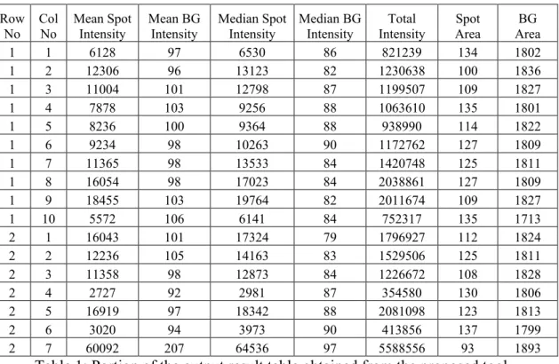
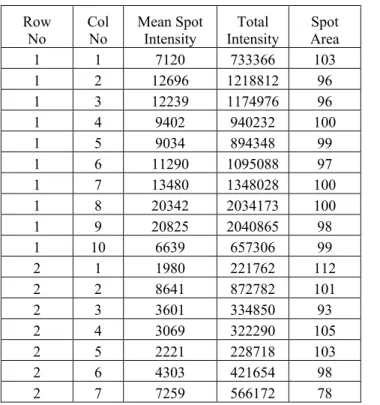
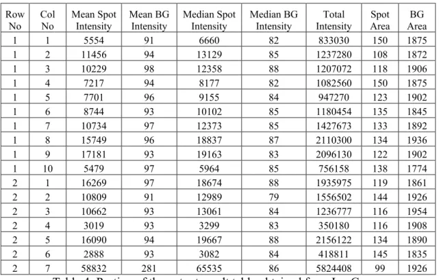
Tables 1-4 show a portion of the output result tables from the four tools tested.
Special notice should be paid to the spot area. In both ScanAlyze (equal number of
pixels in all spots since fixed circle segmentation is used) and TIGR SpotFinder, this
area is smaller than the one found by the tool developed here. This can be easily
belonging to the spots are not detected, hence, the resulting mean, median and mode
intensities are not properly calculated.
Row No Col No Mean Spot Intensity Mean BG Intensity Median Spot Intensity Median BG Intensity Total Intensity Spot Area BG Area
1 1 6128 97 6530 86 821239 134 1802 1 2 12306 96 13123 82 1230638 100 1836 1 3 11004 101 12798 87 1199507 109 1827 1 4 7878 103 9256 88 1063610 135 1801 1 5 8236 100 9364 88 938990 114 1822 1 6 9234 98 10263 90 1172762 127 1809 1 7 11365 98 13533 84 1420748 125 1811 1 8 16054 98 17023 84 2038861 127 1809 1 9 18455 103 19764 82 2011674 109 1827 1 10 5572 106 6141 84 752317 135 1713 2 1 16043 101 17324 79 1796927 112 1824 2 2 12236 105 14163 83 1529506 125 1811 2 3 11358 98 12873 84 1226672 108 1828 2 4 2727 92 2981 87 354580 130 1806 2 5 16919 97 18342 88 2081098 123 1813 2 6 3020 94 3973 90 413856 137 1799 2 7 60092 207 64536 97 5588556 93 1893
Table 1: Portion of the output result table obtained from the proposed tool
Row
No Col No Mean SpotIntensity Mean BGIntensity Median BGIntensity Area Spot Area BG
1 1 7278 168 85 97 1584 1 2 12654 99 86 97 1584 1 3 12166 114 90 97 1584 1 4 9542 190 86 97 1584 1 5 9203 130 87 97 1584 1 6 11293 144 87 97 1584 1 7 12945 201 85 97 1584 1 8 19181 253 90 97 1584 1 9 19579 217 86 97 1584 1 10 6526 181 89 97 1584 1 1 19442 128 89 97 1584 1 2 14594 177 83 97 1584 1 3 12327 118 85 97 1584 1 4 3350 108 85 97 1584 1 5 21252 150 89 97 1584 1 6 3624 132 86 97 1584 1 7 53080 749 89 97 1584
Row
No Col No Mean Spot Intensity Intensity Total Area Spot 1 1 7120 733366 103 1 2 12696 1218812 96 1 3 12239 1174976 96 1 4 9402 940232 100 1 5 9034 894348 99 1 6 11290 1095088 97 1 7 13480 1348028 100 1 8 20342 2034173 100 1 9 20825 2040865 98 1 10 6639 657306 99 2 1 1980 221762 112 2 2 8641 872782 101 2 3 3601 334850 93 2 4 3069 322290 105 2 5 2221 228718 103 2 6 4303 421654 98 2 7 7259 566172 78
Table 3: Portion of the output result table obtained from TIGR SpotFinder
However, this area is larger in the output results found by ImaGene. This leads to
considering some background pixels belonging to the foreground, hence leading to the
corruption of the statistical data. Since, spot segmentation algorithms in ImaGene are
not fully described, this tool was tested using its corresponding results.
Testing the different tools we may conclude that firstly, they do not offer a fully
automatic software, which can process images without user intervention. Secondly,
methods and algorithms used in segmentation of spots do not locate all the pixels
belonging to a spot or sometimes include some of the pixels contributing to the
background. The latter case can damage the result of the analysis. However, the
software tool developed here works automatically, allows user intervention (if
Row
No Col No Mean Spot Intensity Mean BG Intensity Median Spot Intensity Median BG Intensity Intensity Total Area Spot Area BG 1 1 5554 91 6660 82 833030 150 1875 1 2 11456 94 13129 85 1237280 108 1872 1 3 10229 98 12358 88 1207072 118 1906 1 4 7217 94 8177 82 1082560 150 1875 1 5 7701 96 9155 84 947270 123 1902 1 6 8744 93 10102 85 1180454 135 1845 1 7 10734 97 12373 85 1427673 133 1892 1 8 15749 96 18837 87 2110300 134 1936 1 9 17181 93 19163 83 2096130 122 1902 1 10 5479 97 5964 85 756158 138 1774 2 1 16269 97 18674 88 1935975 119 1861 2 2 10809 91 12989 79 1556502 144 1926 2 3 10662 93 13061 84 1236777 116 1954 2 4 3019 93 3299 83 350180 116 1908 2 5 16090 94 19667 88 2156122 134 1890 2 6 2888 93 3082 84 418811 145 1835 2 7 58832 281 65535 86 5824408 99 1926
Table 4: Portion of the output result table obtained from ImaGene
The features of the spot consist of the mean, median and mode of the intensities of the
pixels composing the signal (foreground) and the background, along with the total
intensities for the pixels composing the spot and the background are all tabulated in
the output result. The spot area and perimeter (which are used to calculate the
compactness of the spot) are followed by the circularity value in the output table.
Other outputs of this tool are the Canny and LoG edge detected images and also the
circle-detected image. There is an option for the non-uniform grid to be positioned
over the image, which should be selected prior to the start of the image processing
algorithms.
9 Conclusions
This work presented and discussed the methods and algorithms along with test results
in the development of a microarray image processing and analysis tool. The tool was
It first proposed an algorithm for automatically locating spots on the image leading to
the superimposition of a non-uniform grid over the image. The scheme used
morphological opening as both a smoothing operator and also to preserve circularly
shaped objects in the image. Next, the system used both adaptive shape and circle
segmentation techniques. The fluorescent intensities of these spots were then
extracted and these were recorded in a table along with other feature quality analysis
parameters such as mean, median and mode intensities, signal and background area
and compactness of the shape detected.
Finally, the tool developed was compared against three other tools to determine the
advantages/disadvantages of the former over these tools. The most important
difference was found to be the fact that the tool developed here is fully automatic,
whereas the three tools tested needed user intervention especially in determining and
placing a grid over the image. The other main difference was in the techniques used in
segmenting spots, where the other tools failed to fully segment all the pixels
composing a spot, and in some cases even some of the background was detected as
belonging to a spot.
There are various avenues for potential continuation and improvement of the work
presented here. There exist some images of reduced quality in terms of the presence
of potential spots. In these images apart from noise, some cDNAs are not detected and
hence the image provides a poor estimate of spot numbers. On the other hand, the
gridding algorithm proposed in this contribution depends on the accumulation of spots
this aspect causes a problem for images with more than half the number of possible
spots missing in addressing and locating spots.
Another area of improvement follows spot detection. Currently, the proposed tool
only removes background, i.e., noise that is not attached to spots. This needs to be
rectified so that noise contributing to spot pixel intensities is eliminated from the final
output result. Further analysis of the histogram statistics of each spot would provide a
means for suppressing erroneous information.
In spot segmentation, other techniques should be considered. One such technique is
seeded region growing (SRG) (Adams and Bischof, 1994). The problem faced in this
algorithm is the method of automatic seed selection. Alternatively, pulsed coupled
neural networks (PCNN) (Kuntimad and Ranganath, 1999) have been utilised in
image segmentation. The general approach to segment images using PCNN is to
adjust the parameters of the network so that the neurons corresponding to the pixels of
a given region pulse together and the neurons corresponding to the pixels of adjacent
regions do not pulse together.
References
R. Adams and L. Bischof, “Seeded region growing,” IEEE Transactions on Pattern
Analysis and Machine Intelligence, pp. 641-647, vol. 16, No. 6, 1994.
P. Arabie, L. J. Hubert and G. De Soete, “Clustering and classification”, World
J. Baek, Y.S. Song, G.J. McLachlan, “Segmentation and intensity estimation of
microarray images using a gamma-t mixture model”, Bioinformatics, Vol. 23, No. 4,
pp. 458-465, 2007.
D. H. Ballard and C. M. Brown, “Computer Vision”, Prentice-Hall, 1982.
S. Beucher and F. Meyer, “The morphological approach to segmentation: the
watershed transformation,” Mathematical morphology in image processing, vol. 34 of
Optical Engineering, pages 433-481, Marcel Dekker, New York, 1993.
BioDiscovery, Inc., “ImaGene 4.1,” user’s manual, 2001.
J. Buhler, T. Ideker and D. Haynor, “Dapple: Improved techniques for finding spots
on DNA microarrays,” UW CSE technical report UWTR, 2000.
J. F. Canny, “Finding edges and lines in images”, Technical Report AI-TR-720, MIT,
Artificial Intelligence Laboratory, Cambridge, MA, 1983.
J. F. Canny, “A computational approach to edge detection”, IEEE Transactions on
Pattern Analysis and Machine Intelligence, pp. 679-698, vol. 8, 1986.
I. J. Cox, S. L. Hingorani and S. B. Rao, “A maximum likelihood stereo algorithm”,
Computer Vision and Image Understanding, pp. 542-567, Vol. 63, No. 3, May 1996.
M. B. Eisen, “ScanAlyse documentation,” 1999.
O. Demirkaya, M.H. Asyali, M.M. Shoukri, “Segmentation of cDNA microarry spots
using Markov random field modelling”, Bioinformatics, Vol. 21, No. 13, pp.
2994-3000, 2005.
M. B. Eisen and P. O. Brown, “DNA arrays or analysis of gene expression”, Methods
in Enzymology, 303, 1999.
F. Flett, D. Jungmann-Campello, V. Mersinias, S.L.-M. Koh, R. Godden, and C.P.
the linear chromosome of Streptomyces coelicolor A3(2)" Mol Microbiol, pp.
949-958, vol. 31, 1999.
G. Gerig and F. Klein, “Fast contour identification through efficient Hough Transform
and simplified interpretation strategy”, 8th International Joint Conference on Pattern
Recognition, Paris, pp. 498-500, 1986.
R. Gottardo, J. Besag, M. Stephens and A. Murua, “Probabilistic segmentation and
intensity estimation for microarray images”, Biostatistics, Vol. 7, No. 1, pp. 85-99,
2006.
J. Y. Goulermas, P. Liatsis and M. Johnson, “Real-time intelligent vision systems for
process control”, Proceeding of 4th IchemE Conference on Advances in Process
Control, York, pp. 69-76, 1995.
K. Groch, A. Kuklin, A. Petrov and S. Shams, “Image segmentation and quality
control measures in microarray image analysis”, JALA, vol. 6, no. 3, July 2001.
GSI Lumonics, “QuantArray analysis software,” Operator’s Manual, 1999.
P. V. C. Hough, “Methods and means for recognising complex patterns”, US Patent
3069654, 1962.
J.P. Hua, Z.M. Liu, Z.X. Xiong, Q. Wu and K.R. Castleman, “Microarray BASICA:
Background adjustment, segmentation, image compression and analysis of microarry
images”, EURASIP J Applied Signal Processing, Vol. 1, pp. 92-107, 2004.
J. Illingworth and J. Kittler, “A survey of the Hough Transform”, Computer Vision
Graphics and Image Processing, pp. 87-116, vol. 44, 1988.
J. H. Kim, H. Y. Kim and Y. S. Lee, “A novel method using edge detection for signal
extraction from cDNA microarray image analysis”, Experimental and Molecular
A. Kuklin, “Automation in microarray image analysis with AutoGene”, JALA, vol. 5,
Nov. 2000.
G. Kuntimad and H. S. Ranganath, “Perfect image segmentation using pulsed coupled
neural networks”, IEEE Transactions on Neural Networks, Vol. 10, No. 3, May 1999.
P. Liatsis, “Intelligent visual inspection of manufacturing components”, Ph.D. Thesis,
UMIST, UK, 2002.
R. Lukac and K.N. Plataniotis, “cDNA microarray image segmentation using root
signals”, Int J Imaging Systems and Technology, Vol. 16, No. 2, pp. 51-64, 2006.
R. Nagarajan and M. Upreti, “Correlation statistics for cDNA microarray image
analysis”, IEEE-ACM Trans. Computational Biology and Bioinformatics, Vol. 3, No.
3, pp. 232-238, 2006.
N. Otsu, “A threshold selection method from grey-level histograms”, IEEE Trans.
Systems, Man and Cybernetics, pp. 62-66, vol. 9, 1979.
A. Petrov and S. Shams, “Microarry image processing and quality control”, J VLSI
Signal Processing Systems for Signal, Image and Video Technology, Vol. 38, No. 3,
pp. 211-226, 2004.
J. Rahnenfuhrer, “Image analysis for cDNA microarrays”, Methods of Information in
Medicine, Vol. 44, No. 3, pp. 405-407, 2005.
J. Schalkoff, “Digital Image Processing and Computer Vision”, J. Wiley and Sons,
1989.
P. Soille, “Morphological Image Analysis: Principles and Applications”, Springer,
1999.
TIGR SpotFinder, “http://www.tigr.org/software/tm4/”, for software and
L. Vincent and P. Soille, “Watersheds in digital spaces: An efficient algorithm based
on immersion simulations”, IEEE Transactions on Pattern Analysis and Machine
Intelligence, pp. 583-598, vol. 13, 1991.
P. E. Wellstead and M. B. Zarrop, “Self tuning systems: control and signal
processing”, Wiley, 1991.
Y. H. Yang, M. J. Buckley, S. Dudoit and T. P. Speed, “Comparison methods for
image analysis on cDNA microarray data”, Technical report # 584, Nov. 2000.
Z. Z. Zhou, J. A. Stein and Q. Z. Ji, “GLEAMS: A novel approach to high throughput
genetic micro-array image capture and analysis”, Proceedings of SPIE vol. 4266,
2001.
Biographical notes
Dr Panos Liatsis is a Senior Lecturer and the Director of the Information and
Biomedical Engineering Centre at City University, London. He obtained his first
degree in Electrical Engineering from the University of Thrace and his PhD from the
Control Systems Centre, Department of Electrical Engineering and Electronics at
UMIST. His research interests are in the areas of pattern recognition, image analysis
and intelligent systems, with applications to biomedical engineering. He has published
over 100 papers in the proceedings of international conferences and high-impact
factor international journals. He is a member of the IEE, the IMC and the IEEE.
Mr Mohammed Ali Nazarboland is a PhD student in the Department of Textiles and
Paper in the University of Manchester. He obtained his first degree in Computer
Systems Engineering and his MPhil from the Control Systems Centre, Department of
Electrical Engineering and Electronics, at UMIST. His research interests are in the
areas of image processing and analysis, mathematical modelling and computer
graphics.
Dr John Yannis Goulermas graduated with a first class honours degree in computation
from UMIST in 1994. He received the MSc by research and the PhD degrees in
Electrical Engineering and Electronics at UMIST in 1996 and 2000, respectively. He
worked in the Centre for Virtual Environments and the Centre for Rehabilitation and
Human Performance Research of the University of Salford before joining the
as a Lecturer. His main research interests include pattern recognition, data analysis,
artificial intelligence, machine vision and optimisation.
Dr Xiao-Jun Zeng Dr Zeng joined UMIST in October 2002. Before that, he was with
Knowledge Support Systems Ltd (KSS) from February 1996 to September 2002
where he was a scientific developer, a senior scientific developer and the head of
research. In KSS, he had involved in the research and development of several
intelligent pricing decision support systems. He is a reviewer for IEEE Transaction on
Fuzzy Systems, IEEE Transaction on Systems, Man and Cybernetics, International
Journal of Intelligent and Fuzzy Systems and IFAC Automatica etc. He has published
more than thirty papers in academic journals and conferences.
Dr Efstathios Milonidis received his first degree in Electrical Engineering from the
National Technical University of Athens, his MSc in Control Engineering and his
MPhil in Aerodynamics and Flight Mechanics from Cranfield Institute of
Technology, and his PhD in Control Theory and Design from City University. He is
currently a Lecturer in Control Engineering at the School of Engineering and
Mathematical Sciences at City University. His main research interests are Discrete
Time Control, Modelling and Simulation of Dynamical Systems, Systems Theory and
Figure Legends
Figure 1: Image showing different methods of background adjustments. The
region inside the red circle represents the spot mask and the other regions
bounded by coloured lines represent regions used for local background
calculation by different methods. Green: used in QuantArray; blue: used in
ScanAlyze; and pink: used in Spot (Yang et al., 2000).
Figure 2: Microarray expression of Streptomyces coelicolor.
Figure 3: Overall system structure for the microarray image analysis tool.
Figure 4: Breakdown of the steps in the task of addressing in the microarray image
analysis tool.
Figure 5: Image thresholded with a value (a) 100 (b) 300 (c) 600 (d) 900.
Figure 6: Noise removal using opening (a) Original image (b) Noise preserved
(c) noise removed by using difference image.
Figure 7: Effect of noise filtering (a) Original image, (b) Result of opening
transformation.
Figure 9: Clustering tree structure using the short distance linking method.
Figure 10: The four clusters indicating the four meta-arrays.
Figure 11: The non-uniform grid superimposed on the (a) original image, (b)
opened binary image.
Figure 12: The non-uniform grid superimposed on the image.
Figure 13: Overview of spot segmentation process.
Figure 14: GHTG Circle Detection, different peak size thresholds (a) 2500 (b)
1100 (c) 900.
Figure 15: (a) Original LoG edge detected image (b) different colours indicate;
red: foreground/pixel area, blue: background area, white: vignette surrounding
the spot and grey: edges of the spot.
Figure 16: A testing image showing a meta-grid of 10x10 possible spots.
Figure 17: Grids on the ScanAlyse tool are shown as red circles overlaying the
image. These are also used for segmenting the spot, however, (a) is smaller than
(b) and some parts of the spot in (b) are not contributing to the spot intensity
Figure 18: Comparison of segmentation (a) using TIGR SpotFinder (red line
shows the segmentation area) and (b) the tool developed (black line shows the
Feature Extraction Segmentation
Addressing
Grid Location
Circle Centre Location
Binary Edge Detected Output
Mean Mode Median
Compactness
Background/ Foreground Intensity Original
Image