Approximate Bayesian Computation by Subset Simulation
Manuel Chiachioa,∗, James L. Beckb, Juan Chiachioa, Guillermo Rusa
aDept. Structural Mechanics and Hydraulic Engineering, University of Granada.
Campus de Fuentenueva s/n, 18071 Granada, Spain.
bDivision of Engineering and Applied Science, Mail Code 9-94, California Institute of Technology, Pasadena, CA 91125,
USA.
Abstract
A new Approximate Bayesian Computation (ABC) algorithm for Bayesian updating of model parameters is proposed in this paper, which combines the ABC principles with the technique of Subset Simulation
for efficient rare-event simulation, first developed in S.K. Au and J.L. Beck [1]. It has been named ABC-SubSim. The idea is to choose the nested decreasing sequence of regions in Subset Simulation as the regions that correspond to increasingly closer approximations of the actual data vector in observation space. The efficiency of the algorithm is demonstrated in two examples that illustrate some of the challenges faced in real-world applications of ABC. We show that the proposed algorithm outperforms other recent sequential ABC algorithms in terms of computational efficiency while achieving the same, or better, measure of ac-curacy in the posterior distribution. We also show that ABC-SubSim readily provides an estimate of the evidence (marginal likelihood) for posterior model class assessment, as a by-product.
Keywords: Approximate Bayesian computation, Subset Simulation, Bayesian inverse problem
1. Introduction
The main goal of Bayesian statistics is to update a priori information about the parameter of interestθ∈ Θ⊂Rd for a parameterized model classM, based on the information contained in a set of data which we express as a vectory∈ D ⊂R`, whereDis theobservation space, the region inR`of all possible observational outcomes according to the model class. As a part of the model classM, we choose a prior probability density function (PDF)p(θ|M) over the parameter space and we also derive p(y|θ,M), the likelihood function of
θ, from the stochastic forward model p(x|θ,M) of the model classM[2]. Bayes’ Theorem then yields the posterior PDFp(θ|y,M) of the model specified byθ as follows:
p(θ|y,M) =R p(θ|M)p(y|θ,M) Θp(θ|M)p(y|θ,M)dθ
∝p(θ|M)p(y|θ,M) (1)
However, evaluation of the normalizing integral in the denominator is usually intractable except in some special cases. Also, there are situations where Bayesian analysis is conducted with a likelihood function that is not completely known or it is difficult to obtain, perhaps because it requires the evaluation of an intractable multi-dimensional integral over a latent vector, such as in hidden Markov models or dynamic state-space models, or because the normalization in the likelihood over the observation spaceDinvolves an intractable integral parameterized by θ [3]. Approximate Bayesian Computation (ABC) algorithms were conceived with the aim of evaluating the posterior density in those cases where the likelihood function is intractable
∗Corresponding author. e-mail: [email protected]
Tel: (+34)958240037 Fax: (+34)958249959. E.T.S Ingenieros de Caminos, CC. y PP.
[4, 5], although it also avoids the problem of the intractable integral in Equation 1. In the literature, these classes of algorithms are also called likelihood-free computation algorithms, which refers to their main aim of circumventing the explicit evaluation of the likelihood by using a simulation-based approach. In this introductory section, we briefly summarize the body of ABC literature with a brief description of the main concepts and algorithms that we will need in the subsequent sections.
Let x∈ D ⊂ R` denote a simulated dataset from p(·|θ,M), the forward model of model class M. An ABC algorithm aims at evaluating the posteriorp(θ|y,M)∝p(y|θ,M)p(θ|M) by applying Bayes’ Theorem to the pair (θ, x):
p(θ, x|y)∝p(y|x, θ)p(x|θ)p(θ) (2) In the last equation, the conditioning on model classMhas been omitted for clarity, given that the theory is valid for any specific model class. The functionp(y|x, θ) gives higher weights for the posterior in those regions wherexis close toy. The basic form of the algorithm to sample from the posterior given by Equation 2, is a rejection algorithm that consists of generating jointlyθ∼p(θ) andx∼p(x|θ) and accepting them conditional on fulfilling the equalityx=y. Of course, obtaining samplex=y is unlikely in most applications, and it is only feasible ifDconsists of a finite set of values rather than a region inR`. Hence two main approximations have been conceived in ABC theory to address this difficulty [6]: a) replace the equality x = y by the approximationx≈y and introduce a tolerance parameter that accounts for how close they are through some type of metricρ; and b) introduce a low-dimensional vector of summary statisticsη(·) that permits a comparison of the closeness ofxand y in a weak manner. Through this approach, the posteriorp(θ, x|y) in Equation 2 is approximated by p(θ, x|y), which assigns higher probability density to those values of (θ, x)∈Θ× D that satisfy the conditionρ η(x), η(y)6.
The standard version of the ABC algorithm takes the approximate likelihood1 P(y|θ, x) = P(x ∈ N(y)|x), where N(y) =
x ∈ D : ρ η(x), η(y)
6 . From Bayes’ Theorem, the approximate poste-riorp(θ, x|y) =p θ, x|x∈ N(y)is given by:
p(θ, x|y)∝P(x∈ N(y)|x)p(x|θ)p(θ) (3)
where P(x ∈ N(y)|x) = IN(y)(x), an indicator function for the set N(y) that assigns a value of 1 when ρ η(x), η(y)
6 and 0 otherwise. So the output of the ABC algorithm corresponds to samples from the joint probability density function:
p(θ, x|y)∝p(x|θ)p(θ)IN(y)(x) (4)
with ultimate interest typically being in the marginal approximate posterior:
p(θ|y)∝p(θ) Z
D
p(x|θ)IN(y)(x)dx=P(x∈ N(y)|θ)p(θ) (5)
This integration need not be done explicitly since samples from this marginal PDF are obtained by taking theθcomponent of samples from the joint PDF in Equation 4 [7]. Notice that the quality of the posterior approximation in Equations 4 and 5 depends on a suitable selection of the metricρ, the tolerance parameter
and, of special importance, the summary statistic η(·) [8]. A pseudocode to generate N samples by the standard version of ABC algorithm is given in Algorithm 1.
The choice of tolerance parameter is basically a matter of the amount of computational effort that the user wishes to expend but a possible guiding principle is described later at the end of §3.1.2. For
sufficiently small ( → 0), η(x) → η(y), and so all accepted samples corresponding to Equation 5 come from the closest approximation to the required posterior density p(θ|y), where the exactness is achieved whenη(·) is a sufficient statistic. This desirable fact is at the expense of a high computational effort (usually prohibitive) to getη(x) =η(y) under the modelp(x|θ). On the contrary, as→ ∞, all accepted observations come from the prior. So, the choice ofreflects a trade-off between computability and accuracy.
Algorithm 1Standard ABC fort= 1 toN do
repeat
1.- Simulateθ0 fromp(θ)
2.- Generatex0∼p(x|θ0)
untilρ η(x0), η(y)
6
Accept (θ0, x0) end for
Several computational improvements have been proposed addressing this trade-off. In those cases where the probability content of the posterior is concentrated over a small region in relation to a diffuse prior, the use of Markov Chain Monte Carlo methods (MCMC) [9–11] has been demonstrated to be efficient [6]. In fact, the use of a proposal PDF q(·|·) over the parameter space allows a new parameter to be proposed based on a previous accepted one, targeting the stationary distribution p(θ|y). The resulting algorithm, commonly called ABC-MCMC, is similar to the standard one (Algorithm 1) with the main exception being the acceptance probability, which in this case is influenced by the MCMC acceptance probability as follows:
Algorithm 2ABC-MCMC
1.- Initialize (θ(0), x(0)) fromp
(θ, x|y); e.g. use Algorithm 1. forn= 1 toN do
2.- Generateθ0∼q(θ|θ(n−1)) andx0∼p(x|θ0).
3.- Accept (θ0, x0) as (θ(n), x(n)) with probability:
α= min
1,P(y|x(n−1)P(y|,θx0(n−1),θ0)p()θp0()θq(n−1)(θ(n−1))q(|θθ00|)θ(n−1))
elseset (θ(n), x(n)) = (θ(n−1), x(n−1)) end for
WhenP(y|x, θ) =IN(y)(x), as in our case, the acceptance probabilityαis decomposed into the product of the MCMC acceptance probability and the indicator function:
α= min
1, p(θ
0)q(θ(n−1)|θ0) p(θ(n−1))q(θ0|θ(n−1))
IN(y)(x
0) (6)
In this case, Step 3 is performed only ifx0∈ N
(y). The efficiency of this algorithm is improved with respect to the Standard ABC algorithm, but Equation 6 clearly shows that the dependence uponin the indicator function may lead to an inefficient algorithm for a good approximation of the true posterior. In fact, given that αcan only be non-zero if the eventρ η(x0), η(y)6 occurs, the chain may persist in distributional tails for long periods of time ifis sufficiently small, due to the acceptance probability being zero in Step 3 of Algorithm 2.
Some modifications to the ABC-MCMC scheme have been proposed [12] that provide a moderate im-provement in the simulation efficiency. See [13] for a complete tutorial about ABC-MCMC. More recently, to overcome this drawback associated with ABC-MCMC, a branch of computational techniques have emerged to obtain high accuracy (→ 0) with a feasible computational burden by combining sequential sampling algorithms [14] adapted for ABC. These techniques share a common principle of achieving computational ef-ficiency by learning about intermediate target distributions determined by a decreasing sequence of tolerance levels1> 2> . . . > m=, where the last is the desired tolerance. Table 1 lists the main contributions to the literature on this topic. However, more research is needed to perform posterior simulations in a more efficient manner.
Simulation [1, 15, 16] to achieve computational efficiency in a sequential way. The main idea is to link an ABC algorithm with a highly-efficient rare-event sampler that draws conditional samples from a nested sequence of subdomains defined in an adaptive and automatic manner. ABC-SubSim can utilize many of the improvements proposed in the recent ABC literature because of the fact that the algorithm is focused on the core simulation engine.
The paper is organized as follows. Section 2 reviews the theory underlying Subset Simulation and then the ABC-SubSim algorithm is introduced in Section 3. The efficiency of ABC-SubSim is illustrated in Section 4 with two examples of dynamical models with synthetic data. In Section 5, the performance of the algorithm is compared with some others in the recent ABC literature and the use of ABC-SubSim for posterior model class assessment is discussed. Section 6 provides concluding remarks.
2. Subset Simulation method
Subset Simulation is a simulation approach originally proposed to compute small failure probabilities encountered in reliability analysis of engineering systems (e.g. [1, 15, 17]). Strictly speaking, it is a method for efficiently generating conditional samples that correspond to specified levels of a performance function
g:Rd →
Rin a progressive manner, converting a problem involving rare-event simulation into a sequence of problems involving more frequent events.
LetF be the failure region in thez-space,z∈Z ⊂Rd, corresponding to exceedance of the performance function above some specified threshold levelb:
F ={z∈Z:g(z)> b} (7)
For simpler notation, we useP(F)≡P(z∈F). Let us now assume thatF is defined as the intersection of
mregionsF =Tm
j=1Fj, such that they are arranged as a nested sequenceF1⊃F2. . .⊃Fm−1 ⊃Fm=F, where Fj ={z ∈ Z : g(z)> bj}, with bj+1 > bj, such that p(z|Fj)∝p(z)IFj(z), j = 1, . . . , m. The term p(z) denotes the probability model forz. When the eventFj holds, then{Fj−1, . . . , F1}also hold, and hence
P(Fj|Fj−1, . . . , F1) =P(Fj|Fj−1), so it follows that:
P(F) =P m \
j=1
Fj
=P(F1) m Y
j=2
P(Fj|Fj−1) (8)
whereP(Fj|Fj−1)≡P(z∈Fj|z∈Fj−1), is the conditional failure probability at the (j−1)th conditional level. Notice that although the probability P(F) can be relatively small, by choosing the intermediate regions appropriately, the conditional probabilities involved in Equation 8 can be made large, thus avoiding simulation of rare events.
In the last equation, apart from P(F1), the remaining factors cannot be efficiently estimated by the standard Monte Carlo method (MC) because of the conditional sampling involved, especially at higher intermediate levels. Therefore, in Subset Simulation, only the first probabilityP(F1) is estimated by MC:
P(F1)≈P¯1= 1
N N X
n=1 IF1(z
(n)
0 ), z
(n) 0
i.i.d.
∼ p(z0) (9)
When j > 2, sampling from the PDF p(zj−1|Fj−1) can be achieved by using MCMC at the expense of generatingN dependent samples, giving:
P(Fj|Fj−1)≈P¯j = 1
N N X
n=1 IFj(z
(n)
j−1), z (n)
j−1∼p(zj−1|Fj−1) (10)
Observe that the Markov chain samples that are generated at the (j−1)th level which lie in F j are distributed asp(z|Fj) and thus, they provide “seeds” for simulating more samples according top(z|Fj) by using MCMC sampling with no burn-in required. As described further below,Fjis actually chosen adaptively based on the samples{zj(n−)1, n= 1, . . . , N}fromp(z|Fj−1) in such a way that there are exactlyN P0 of these seed samples in Fj so ¯Pj = P0 in Equation 10. Then a further (1/P0−1) samples are generated from p(z|Fj) by MCMC starting at each seed, giving a total ofN samples in Fj. Repeating this process, we can compute the conditional probabilities of the higher-conditional levels until the final regionFm=F has been reached.
To draw samples from the target PDFp(z|Fj) using the Metropolis algorithm, a suitable proposal PDF must be chosen. In the original version of Subset Simulation [1], a modified Metropolis algorithm (MMA) was proposed that works well even in very high dimensions (e.g. 103-104), because the original algorithm fails in this case (essentially all candidate samples from the proposal PDF are rejected-see the analysis in [1]). In MMA, a univariate proposal PDF is chosen for each component of the parameter vector and each component candidate is accepted or rejected separately, instead of drawing a full parameter vector candidate from a multi-dimensional PDF as in the original algorithm. Later in [15], grouping of the parameters was considered when constructing a proposal PDF to allow for the case where small groups of components in the parameter vector are highly correlated when conditioned on anyFj. An appropriate choice for the proposal PDF for ABC-SubSim is introduced in the next section.
It is important to remark that in Subset Simulation, an inadequate choice of the bj-sequence may lead to the conditional probabilityP(Fj|Fj−1) being very small (if the difference bj−bj−1 is too large), which will lead to a rare-event simulation problem. If, on the contrary, the intermediate threshold values were chosen too close so that the conditional failure probabilities were very high, the algorithm would take a large total number of simulation levelsm (and hence large computational effort) to progress to the target region of interest, F. A rational choice that strikes a balance between these two extremes is to choose the bj-sequence adaptively [1], so that the estimated conditional probabilities are equal to a fixed value P0 (e.g. P0 = 0.2). For convenience, P0 is chosen so that N P0 and 1/P0 are positive integers. For a specified value ofP0, the intermediate threshold value bj defining Fj is obtained in an automated manner as the [(1−P0)N]
th
largest value among the valuesg(z(jn−)1), n= 1, . . . , N, so that the sample estimate of
P(Fj|Fj−1) in Equation 10 is equal toP0.
3. Subset Simulation for ABC
Here we exploit Subset Simulation as an efficient sampler for the inference of rare events by just spe-cializing the Subset Simulation method described in§2 to ABC. To this end, let us definez asz= (θ, x)∈
Z=Θ× D ⊂Rd+`, so thatp(z) =p(x|θ)p(θ). Let alsoFj in§2 be replaced by a nested sequence of regions Dj, j = 1. . . , m, inZ defined by:
Dj= n
z∈Z:x∈ Nj(y) o
≡n(θ, x) :ρ η(x), η(y)6j o
(11)
with Dj ⊂Θ× D and ρis a metric on the set {η(x) :x∈ D}. The sequence of tolerances 1, 2, . . . , m, withj+1< j, will be chosen adaptively as described in§2, where the number of levelsmis chosen so that m6, a specified tolerance.
As stated by Equation 4, an ABC algorithm aims at evaluating the sequence of intermediate posteriors
p(θ, x|Dj), j = 1, . . . , m, where by Bayes’ Theorem:
p(θ, x|Dj) =
P(Dj|θ, x)p(x|θ)p(θ) P(Dj)
∝IDj(θ, x)p(x|θ)p(θ) (12)
convergence to the stationary distribution, as was described in §1 for ABC-MCMC. This is the point at which we exploit the efficiency of Subset Simulation for ABC, given that such a small probabilityP(Dm) is converted into a sequence of larger conditional probabilities, as stated in Equations 8, 9 and 10.
3.1. The ABC-SubSim algorithm
Algorithm 3 provides a pseudocode implementation of ABC-SubSim that is intended to be sufficient for most situations. The algorithm is implemented such that a maximum allowable number of simulation levels (m) is considered in case the specifiedis too small. The choice ofis discussed at the end of §3.1.2.
Algorithm 3Pseudocode implementation for ABC-SubSim Inputs:
P0∈[0,1]{gives percentile selection, chosen soN P0,1/P0∈Z+; P0= 0.2 is recommended}.
N,{number of samples per intermediate level};m,{maximum number of simulation levels allowed} Algorithm:
Sampleh θ(1)0 , x (1) 0
, . . . , θ(0n), x (n) 0
, . . . , θ(0N), x (N) 0
i
, where (θ, x)∼p(θ)p(x|θ) forj: 1, . . . , mdo
forn: 1, . . . , N do Evaluateρ(jn)=ρ η(x
(n) j−1), η(y)
end for
Renumberh θ(jn−)1, x(jn−)1
, n: 1, . . . , Niso thatρ(1)j 6ρ(2)j 6. . . ρ(jN)
Fixj = 12
ρ(N P0)
j +ρ
(N P0+1) j
fork= 1, . . . , N P0do
Select as a seed θ(jk),1, x(jk),1
= θ(jk−)1, x(jk−)1
∼p θ, x|(θ, x)∈Dj
Run Modified Metropolis Algorithm [1] to generate 1/P0 states of a Markov chain lying in Dj (Eq. 11): h θ(jk),1, x
(k),1 j
, . . . , θ(jk),1/P0, x (k),1/P0 j
i
end for
Renumberh(θ(jk),i, x (k),i
j ) :k= 1, . . . , N P0;i= 1, . . . ,1/P0 i
as h
(θ(1)j , x (1)
j ), . . . ,(θ (N) j , x
(N) j )
i
if j 6 then End algorithm end if
end for
3.1.1. Choice of intermediate tolerance levels
In Algorithm 3, the j values are chosen adaptively as in Subset Simulation [1], so that the sample estimate ¯PjofP(Dj|Dj−1) satisfies ¯Pj=P0. By this way, the intermediate tolerance valuej can be simply obtained as the 100P0percentile of the set of distancesρ η(x(
n) j−1), η(y)
3.1.2. Choosing ABC-SubSim control parameters
The important control parameters to be chosen in Algorithm 3 are P0 and σj2, the variance in the Gaussian proposal PDF in MMA at thejthlevel. In this section we make recommendations for the choice of these control parameters.
In the literature, the optimal variance of a local proposal PDF for a MCMC sampler has been studied due to its significant impact on the speed of convergence of the algorithm [19, 20]. ABC-SubSim has the novelty of incorporating the Subset Simulation procedure in the ABC algorithm, so we use the same optimal adaptive scaling strategy as in Subset Simulation. To avoid duplication of literature for this technique but conferring a sufficient conceptual framework, the method for the optimal choice of theσj2 is presented in a brief way. The reader is referred to the recent work of [18], where optimal scaling is addressed for Subset Simulation and a brief historical overview is also given for the topic.
Suppose that the reason for wanting to generate posterior samples is that we wish to calculate the posterior expectation of a quantity of interest which is a functionh:θ∈Θ→R. We consider the estimate of its expectation with respect to the samples generated in each of thejthlevels:
¯
hj =Ep(θ|Dj)[h(θ)]≈ 1
N N X
n=1
h(θ(jn)) (13)
whereθj(n), n= 1, . . . , N are dependent samples drawn from Nc Markov chains generated at thejth condi-tional level. An expression for the variance of the estimator can be written as follows [1]:
Var(¯hj) = R(0)j
N (1 +γj), (14)
with
γj = 2 Ns−1
X
τ=1
Ns−τ Ns
R(τ) j
R(0)j
(15)
In the last equationNs=1/P0 is the length of each of the Markov chains, which are considered probabilisti-cally equivalent [1]. The termR(jτ) is the autocovariance ofh(θ) at lag τ,R
(τ)
j =E
h
h(θj(1))h(θ (τ+1)
j )
i −¯h2
j, which can be estimated using the Markov chain samplesθ(jk),i:k= 1, . . . , Nc;i= 1, . . . , Ns as2:
R(jτ)≈R˜ (τ)
j =
" 1
N−τ Nc Nc X
k=1 Ns−τ
X
i=1
h(θj(k),i)h(θ (k),τ+i
j )
#
−¯h2j (16)
whereNc=N P0, so thatN =NcNs.
Given that the efficiency of the estimator ¯hj is reduced when γj is high, the optimal proposal variance σ2
j for simulation level jth is chosen adaptively by minimizing γj. This configuration typically gives an acceptance rate ¯αfor each simulation level in the range of 0.2-0.4 [18]. This is supported by the numerical experiments performed with the examples in the next section, which leads to our recommendation for ABC-SubSim: Adaptively choose the variance σ2
j of the j
th intermediate level so that the monitored acceptance
rateα¯∈[0.2,0.4]based on an initial chain sample of small length (e.g. 10 states).
The choice of the conditional probabilityP0 has a significant influence on the number of intermediate simulation levels required by the algorithm. The higher P0 is, the higher the number of simulation levels employed by the algorithm to reach the specified tolerance, for a fixed number of model evaluations (N) per simulation level. This necessarily increases the computational cost of the algorithm. At the same time, the
2It is assumed for simplicity in the analysis that the samples generated by the differentN
smallerP0 is, the lower the quality of the posterior approximation, that is, the larger the values of γj in Equation 14. The choice ofP0 therefore requires a trade-off between computational efficiency and efficacy, in the sense of quality of the ABC posterior approximation.
To examine this fact, let us take a fixed total number of samples, i.e. NT =mN, wheremis the number of levels required to reach the target tolerance value , a tolerance for which R(0)m ≈Var [h(θ)]. The value ofm depends on the choice ofP0. We can chooseP0 in an optimal way by minimizing the variance of the estimator ¯hmfor the last simulation level:
Var(¯hm) = Rm(0)
NT/m(1 +γm)∝m(1 +γm) (17)
Notice thatγmalso depends uponP0, although it is not explicitly denoted, as we will show later in§4 (Figure 2). In the original presentation of Subset Simulation in [1],P0= 0.1 was recommended, and more recently in [18], the range 0.16P0 60.3 was found to be near optimal after a rigorous sensitivity study of Subset Simulation, although the optimality there is related to the coefficient of variation of the failure probability estimate. The valueP0= 0.2 for ABC-SubSim is also supported by the numerical experiments performed with the examples in the next section, where we minimize the variance in Equation 17 as a function ofP0, which leads to the recommendation:For ABC-SubSim, set the conditional probabilityP0= 0.2.
Finally, it is important to remark that an appropriate final tolerance may be difficult to specify a priori. For these cases, one recommendation is to select adaptively so that the posterior samples give a stable estimate ¯hm of Ep(θ|Dm)[h(θ)] (Equation 13), i.e. a further reduction in does not change ¯hm significantly.
3.2. Evidence computation by means of ABC-SubSim
In a modeling framework, different model classes can be formulated and hypothesized to idealize the experimental system, and each of them can be used to solve the probabilistic inverse problem in Equation 1. If the modeler chooses a set of candidate model classes M = {Mk, k = 1, . . . , NM}, Bayesian model class assessment is a rigorous procedure to rank each candidate model class based on their probabilities conditional on datay [21, 22]:
P(Mk|y,M) =
p(y|Mk)P(Mk|M) XNM
i=1p(y|Mi)P(Mi|M)
(18)
whereP(Mk|M) is the prior probability of eachMk, that expresses the modeler’s judgement on the initial relative plausibility ofMk withinM. The factorp(y|Mk), which is called theevidence (ormarginal likeli-hood) for the model class, expresses how likely the data y are according to the model class. The evidence
p(y|Mk) is equal to the normalizing constant in establishing the posterior PDF in Equation 1 for the model class3: p(y|M
k) = R
Θp(y|θ,Mk)p(θ|Mk)dθ.
When the likelihood is not available, the evidence p(y|Mk) is approximated using ABC by P(y|Mk), which depends upon, the summary statisticη(·) as well as the chosen metricρ[23]. In terms of the notation in Equation 11, the ABC evidence can be expressed as:
P(y|Mk) =P(Dm|Mk) = Z
Θ
P(Dm|θ, x,Mk)p(x|θ,Mk)p(θ|Mk)dθdx (19)
The evaluation of the last integral is the computationally expensive step in Bayesian model selection, espe-cially when →0 [3]. Observe thatP(y|Mk) in Equation 19 is expressed as a mathematical expectation that can be readily estimated as follows:
P(y|Mk)≈ 1
N N X
n=1 IDm θ
(n), x(n)
(20)
where θ(n), x(n)
∼p(x|θ,Mk)p(θ|Mk) are samples that can be drawn using the Standard ABC algorithm (Algorithm 1), which in this setting is equivalent to the Standard Monte Carlo method for evaluating integrals. The main drawback of this method arises when employing→0, due to the well-known inefficiency of the Standard ABC algorithm. Moreover, the quality of the approximation in Equation 20 may be poor in this situation unless a huge amount of samples are employed because otherwise the Monte Carlo estimator has a large variance. Hence, several methods have emerged in the ABC literature to alleviate this difficulty, with the main drawback typically being the computational burden. See [24] for discussion of this topic.
ABC-SubSim algorithm provides a straight-forward way to approximate the ABC evidence P(y|Mk) via the conditional probabilities involved in Subset Simulation:
P(y|Mk) =P(Dm|Mk) =P(D1) m Y
j=2
P(Dj|Dj−1)≈P0m (21)
The last is an estimator for P(y|Mk) which is asymptotically unbiased with bias O(1/N). See [1, 18] for a detailed study of the quality of the estimators based on Subset Simulation where the approximation is studied in the context of the failure probability estimate (but notice that Equations 21 and 8 are essentially the same). Of course, there are also approximation errors due to the ABC approximation that depend on the choice of, η(·) andρ[23]. Finally, onceP(y|Mk) is calculated, it is substituted forp(y|Mk) in Equation 18 to obtainP(Mk|y,M), the ABC estimate of the model class posterior probability. It is important to remark here that there are well-known limitations of the ABC approach to the model selection problem, typically attributable to the absence of sensible summary statistics that work across model classes, among others [23, 24]. Our objective here is to demonstrate that calculation of the ABC evidence is a simple by-product of ABC-SubSim, as given in Equation 21.
4. Illustrative examples
In this section we illustrate the use of ABC-SubSim with two examples: 1) a moving average process of orderd= 2, MA(2), previously considered in [3]; 2) a single degree-of-freedom (SDOF) linear oscillator subject to white noise excitation, which is an application to a state-space model. Both examples are input-output type problems, in which we adopt the notationy= [y1, . . . , yl, . . . , y`] for the measured system output sequence of length`. The objective of these examples is to illustrate the ability of our algorithm to be able to sample from the ABC posterior for small values of. In the MA(2) example, we take for the metric the quadratic distance between thed= 2 first autocovariances, as in [3]:
ρ η(x), η(y) =
d X
q=1
(τy,q−τx,q)2 (22)
In the last equation, the terms τy,q and τx,q are the autocovariances of y and x, respectively, which are used as summary statistics. They are obtained asτy,q =P
`
k=q+1ykyk−q andτx,q=P `
k=q+1xkxk−q, respec-tively. The Euclidean distance ofxfrom y is considered as the metric for the oscillator example:
ρ(x, y) = " `
X
l=1
(yl−xl)2 #1/2
(23)
To evaluate the quality of the posterior, we study the variance of the mean estimator of a quantity of interest
h:θ∈Θ→R, defined as follows (see§3.1.2):
h(θ) = d X
i=1
θi 2
4.1. Example 1: Moving Average (MA) model
Consider a MA(2) stochastic process, withxl, l= 1, . . . , `, the stochastic variable defined by:
xl=el+ d X
i=1
θiel−i (25)
with d= 2, ` = 100 or 1000. Here e is an i.i.d sequence of standard Gaussian distributions N(0,1): e = [e−d+1, . . . , e0, e1. . . el, . . . , e`] and x = [x1, . . . , xl, . . . , x`]. To avoid unnecessary difficulties, a standard identifiability condition is imposed on this model [3], namely that the roots of the polynomial D(ξ) = 1−Pd
i=1θiξi are outside the unit circle in the complex plane. In our case ofd= 2, this condition is fulfilled when the regionΘ is defined as all (θ1, θ2) that satisfy:
−2< θ1<2;θ1+θ2>−1;θ1−θ2<1 The prior is taken as a uniform distribution overΘ.
Note that, in principle, this example does not need ABC methods as the likelihood is a multidimensional Gaussian with zero mean and a covariance matrix of order ` that depends on (θ1, θ2), but its evaluation requires a considerable computational effort when ` is large [25]. This example was also used to illustrate the ABC method in [3] where it was found that the performance is rather poor if the metric is the one in Equation 23 which uses the “raw” data but ABC gave satisfactory performance when the metric in Equation 22 was used. For comparison with Figure 1 [3], we also choose the latter here.
We use synthetic data foryby generating it from Equation 25 consideringθtrue= (0.6,0.2). The chosen values of the control parameters for ABC-SubSim are shown in Table 2. The ABC-SubSim results are presented in Figure 1, which shows that the mean estimate of the “approximate” posterior samples at each level is close toθtrue, for both`= 100 and`= 1000 cases. Figure 1a shows the case `= 100 which can be compared with Figure 1 in [3]. In Figure 1a, a total of 3000 samples were used to generate 1000 samples to represent the posterior, whereas in [3], 1,000,000 samples were used to generate 1000 approximate posterior samples using the standard ABC algorithm that we called Algorithm 1. The ABC-SubSim posterior samples give a more compact set that is better aligned with the exact posterior contours given in Figure 1 of [3]. Figure 1b shows that for the case`= 1000, ABC-SubSim used 4000 samples to generate 1000 samples representing the much more compact posterior that corresponds to ten times more data.
A preliminarily sensitivity study was done to corroborate the choice of the algorithm control parameters described in§3.1.2 and the results are shown in Figure 2. As described in§3.1.2, the optimal value ofP0 is the one that minimizesm(1 +γm) for fixed tolerance. As an exercise, we consider= 1.12·104as the final tolerance.4 The results in Figure 2 show thatP0= 0.2 is optimal since thenm(1 +γm) = 3(1 + 2.8) = 11.4; whereas forP0= 0.5 andP0= 0.1, it is 7(1 + 0.86) = 13.1 and 2(1 + 5.1) = 12.2, respectively. These results are consistent with those for rare event simulation in [18]. Observe also that the optimal varianceσ2
j for the Gaussian proposal PDF at the jth level that minimizes γ
j occurs when the acceptance rate ¯αj in MMA lies in the range 0.2-0.4, which is also consistent with that found in [18] (except for the case of very low acceptance rate where the process is mostly controlled by the noise).
4.2. Example 2: Linear oscillator
Consider the case of aSDOFoscillator subject to white noise excitation as follows:
mξ¨+cξ˙+kξ=f(t) (26) whereξ=ξ(t)∈R[m], m[Kg], k[N/m] andc[N·s/m] are the displacement, mass, stiffness and damping coefficient, respectively. To construct synthetic input, a discrete-time history of input forcef [N] modeled by Gaussian white noise with spectral intensitySf = 0.0048 [N2·s], is used. The time step used to generate
4It is unlikely that one or more values from the-sequence obtained using differentP
0 values coincide exactly. Hence, the
the input data is 0.01 [s], which gives an actual value for the variance of the discrete input forceσ2
f= 3 [N] [26, 27].
The probability model that gives the likelihood function of this example is Gaussian and so it can be written explicitly although its evaluation requires the computation of a high dimensional matrix inverse [28]. Repeated evaluations of the likelihood function for thousands of times in a simulation-based inference process is computationally prohibitive for large-size datasets. However it is easy to simulate datasets from this model after some trivial manipulations of Equation 26 [28]. Therefore, this example is particularly suited for the use of ABC methods.
The mechanical system is assumed to have known mass m= 3 [Kg] and known input force giving the excitation. For the state-space simulation, denote thestate vector bys(t) =hξ(t),ξ˙(t)i
T
. Equation 26 can be rewritten in state-space form as follows:
˙
s(t) =Acs(t) +Bcf(t) (27) whereAc∈R2×2,Bc∈R2×1 are obtained as:
Ac=
0 1
−m−1k −m−1c
Bc=
0
m−1
(28)
By approximating the excitation as constant within any interval, i.e. f(l4t+τ) = f(l4t),∀τ ∈ [0,4t), Equation 27 can be discretized to a difference equation:∀l>1,
sl=Asl−1+Bfl−1 (29)
withsl≡s(l4t),fl≡f(l4t),l= 0,1,2, . . . , `, andA andB are matrices given by:
A=e(Ac4t) (30a)
B =A−1
c (A−I2)Bc (30b)
whereI2 is the identity matrix of order 2. The use of discrete-time input and output data here is typical of the electronically-collected data available from modern instrumentation on mechanical or structural systems. We adoptθ={k, c}as unknown model parameters and denote byylandxlthe vectors consisting of the actual and predicted response measurements at each4t. Samples ofxlfor a given input force time history {fl} andθ, can be readily generated by the underlying state-space model:
sl=Asl−1+Bfl−1+el (31a)
xl= [1,0]sl+e0l (31b)
where el and e0l are error terms to account for model prediction error and measurement noise, respec-tively. Since in reality these errors would be unknown, we use the Principle of Maximum Information Entropy [2, 29, 30] to chooseel and e0l as i.i.d. Gaussian variables,el ∼ N(0, σe2I2), e0l ∼ N(0, σe20) and so they can be readily sampled. For simplicity, we adoptσ2
e= 10−2andσe20 = 10−6, taking them as known. We cally={y1, . . . , yl, . . . , y`}the batch dataset collected during a total period of timet=`4t, starting from known initial conditionss0= [0.01,0.03]T (units expressed in [m] and [m/s] respectively). In this example, the noisy measurementsyl are synthetically generated from Equation 31 for the given input force history and for model parameters θtrue = {k = 4π, c = 0.4π}. We also adopt a sampling rate for the resulting output signal of 100 [Hz] (4t= 0.01[s]) during a sampling period oft = 3[s], hence` = 300. We choose a uniform prior over the parameter spaceΘdefined by the region 0< θi63;i∈ {1,2}. Table 2 provides the information for the algorithm configuration.
5. Discussion
5.1. Comparison with recent sequential ABC algorithms
In this section, ABC-SubSim is compared with a selection of recent versions of sequential ABC algo-rithms: ABC-SMC [31], ABC-PMC [32] and ABC-PT [33], which are listed in Table 1. The same number of evaluations per simulation level are adopted for all algorithms, corresponding to 1000 and 2000 for the MA(2) and SDOF model, respectively. We set the sequence of tolerance levels obtained by ABC-SubSim usingP0= 0.5 for the rest of the algorithms (see Table 3). This was done because the recommended near-optimal value ofP0= 0.2 (see§3.1.2) for ABC-SubSim produced a sequence ofvalues that decreased too quickly for ABC-PMC and ABC-SMC to work properly. We note that this non-optimal choice of P0 for ABC-SubSim and the use of its -sequence provide considerable help for the competing algorithms. The proposal PDFs are assumed to be Gaussian for all of the algorithms.
The results shown in Figure 4 are evaluated over the intermediate posterior samples for each simulation level and were obtained considering the mean of 100 independent runs of the algorithms, a large enough number of runs to ensure the convergence of the mean. In this example, we focus on the number of model evaluations together with the quality of the posterior. The left side of Figure 4 shows the accumulated amount of model evaluations employed by each of the competing algorithms. Note that each algorithm requires the evaluation of auxiliary calculations, like those for the evaluation of particle weights, transition kernel steps, etc. However, this cost is negligible because the vast proportion of computational time in ABC is spent on simulating the model repeatedly. The number of model evaluations for ABC-PMC and ABC-PT is variable for each algorithm run, so in both cases we present the mean (labelled dotted lines) and a 95% band (dashed lines). In contrast, ABC-SubSim and also ABC-SMC make a fixed number of model evaluations at each simulation level. Observe that the computational saving is markedly high when comparing with ABC-PMC. Regarding the quality of the posterior, we consider two measures: a) the sample mean of the quadratic error between ¯θandθtrue, i.e.,kθ¯j−θtruek22, as an accuracy measure; and b) the differential entropy5of the final posterior, by calculating1/2ln|(2πe)ddet [cov(θ
j)]|, as a measure quantifying the posterior uncertainty of the model parameters. The results are shown on the right side of Figure 4. Only the last 4 simulation levels are presented for simplicity and clearness.
This comparison shows that ABC-SubSim gives the same, or better, quality than the rest of the ABC algorithms to draw ABC posterior samples whenis small enough, even though it used a smaller number of model evaluations.
5.2. Evidence calculation
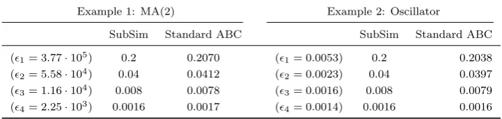
In this section we show how ABC-SubSim algorithm can be applied to estimate the ABC evidence by taking advantage of the improvements in parameter space exploration introduced by Subset Simulation. Ta-ble 4 shows the estimated values of the ABC evidence obtained with the ABC-SubSim algorithm (P0= 0.2), which are computed using a total number of samples per simulation level N equal to 1000 and 2000 for MA(2) and SDOF model, respectively. For each value ofj chosen adaptively by ABC-SubSim as described in §3.1.1, we also calculate the ABC evidence using the approximation in Equation 20 with N = 200,000 samples per value for the Standard ABC algorithm (a large enough amount of samples for the approxi-mation in Equation 20 to be sufficiently accurate). It is seen in both examples that the results obtained by ABC-SubSim and Standard ABC agree well.
These results suggest that if the well-known difficulties of the ABC model choice problem can be ad-equately resolved, high efficiency can be obtained by employing the ABC-SubSim algorithm for the ABC evidence computation.
5This expression for the differential entropy is actually an upper-bound approximation to the actual differential entropy,
6. Conclusions
A new ABC algorithm based on Markov Chain Monte Carlo has been presented and discussed in this paper. This algorithm combines the principles of Approximate Bayesian Computation (ABC) with a highly-efficient rare-event sampler, Subset Simulation, which draws conditional samples from a nested sequence of subdomains defined in an adaptive and automatic manner. We demonstrate the computational efficiency that can be gained with ABC-SubSim by two different examples that illustrate some of the challenges in real-world applications of ABC. The main conclusions of this work are:
• By its construction, ABC-SubSim avoids the difficulties of ABC-MCMC algorithm in initializing the chain, as no burn-in is required.
• In comparison with other recent sequential ABC algorithms, ABC-SubSim requires a smaller number of model evaluations per simulation level to maintain the same quality of the posterior as the other algorithms.
• Together with ABC-SMC from [31], ABC-SubSim does not require the specification of a sequence of tolerance levels, which avoids tedious preliminary calibrations.
• ABC-SubSim allows a straightforward way to obtain an estimate of the ABC evidence used for model class assessment.
Acknowledgments
[1] S. Au, J. Beck, Estimation of small failure probabilities in high dimensions bySubsetSimulation, Probabilistic Engineering Mechanics 16 (4) (2001) 263–277.
[2] J. Beck,Bayesian system identification based on probability logic, Structural Control and Health Monitoring 17 (7) (2010) 825–847.
[3] J. Marin, P. Pudlo, C. Robert, R. Ryder, ApproximateBayesian computational methods, Statistics and Computing 22 (6) (2012) 1167–1180.
[4] S. Tavare, D. Balding, R. Griffiths, P. Donnelly, Inferring coalescence times fromDNAsequence data, Genetics 145 (2) (1997) 505.
[5] J. Pritchard, M. Seielstad, A. Perez-Lezaun, M. Feldman, Population growth of humanY chromosomes: a study of Y chromosome microsatellites., Molecular Biology and Evolution 16 (12) (1999) 1791–1798.
[6] P. Marjoram, J. Molitor, V. Plagnol, S. Tavar´e, Markov chain Monte Carlo without likelihoods, Proceedings of the National Academy of Sciences of the United States of America 100 (26) (2003) 15324–15328.
[7] C. Robert, G. Casella, MonteCarlo statistical methods, 2nd Ed., Springer-Verlag, New York, 2004.
[8] P. Fearnhead, D. Prangle, Constructing summary statistics for approximateBayesian computation: semi-automatic ap-proximateBayesian computation, Journal of the Royal Statistical Society, Series B 74 (3) (2012) 419–474.
[9] W. Gilks, S. Richardson, D. Spiegelhalter,Markov chainMonteCarlo in practice, Chapman and Hall, 1996.
[10] R. Neal, Probabilistic inference usingMarkov chainMonteCarlo methods, Tech. Rep. CRG TR 93 1, Department of Computer Science, University of Toronto, 1993.
[11] W. Gilks,Markov chainMonteCarlo, Wiley Online Library, 2005.
[12] P. Bortot, S. Coles, S. Sisson, Inference for stereological extremes, Journal of the American Statistical Association 102 (477) (2007) 84–92.
[13] S. Sisson, Y. Fan, Handbook ofMarkov chainMonteCarlo, chap. Likelihood-freeMarkov chainMonteCarlo, Chapman and Hall/CRC Press, 319–341, 2011.
[14] P. Del Moral, A. Doucet, A. Jasra, SequentialMonteCarlo samplers, Journal of the Royal Statistical Society: Series B (Statistical Methodology) 68 (3) (2006) 411–436.
[15] S. Au, J. Beck, SubsetSimulation and its application to seismic risk based on dynamic analysis, Journal of Engineering Mechanics 129 (8) (2003) 901–917.
[16] S. Au, J. Ching, J. Beck, Application ofSubsetSimulation methods to reliability benchmark problems, Structural Safety 29 (3) (2007) 183–193.
[17] J. Ching, S. Au, J. Beck, Reliability estimation of dynamical systems subject to stochastic excitation using Subset Simulation with splitting, Computer Methods in Applied Mechanics and Engineering 194 (12-16) (2005) 1557–1579. [18] K. Zuev, J. Beck, S. Au, L. Katafygiotis, Bayesian post-processor and other enhancements of SubsetSimulation for
estimating failure probabilities in high dimensions, Computers & Structures 93 (2011) 283–296.
[19] A. Gelman, G. Roberts, W. Gilks, EfficientMetropolis jumping rules,Bayesian statistics 5 (1996) 599–608.
[20] G. Roberts, J. Rosenthal, Optimal scaling for variousMetropolis-Hastings algorithms, Statistical Science 16 (4) (2001) 351–367.
[21] D. MacKay, Bayesian interpolation, Neural computation 4 (3) (1992) 415–447.
[22] J. Beck, K. Yuen, Model selection using response measurements:Bayesian probabilistic approach, Journal ofEngineering Mechanics 130 (2004) 192.
[23] C. Robert, J. Cornuet, J. Marin, N. Pillai, Lack of confidence in approximate Bayesian computation model choice, Proceedings of the National Academy of Sciences 108 (37) (2011) 15112–15117.
[24] X. Didelot, R. Everitt, A. Johansen, D. Lawson, Likelihood free estimation of model evidence, Bayesian analysis 6 (1) (2011) 49–76.
[25] J. Marin, C. Robert, Bayesian core: a practical approach to computationalBayesian statistics, Springer, 2007. [26] M. Hayes, Statistical digital signal processing and modeling, John Wiley & Sons, 2009.
[27] K. Yuen, J. Beck, Updating properties of nonlinear dynamical systems with uncertain input, Journal of Engineering Mechanics 129 (1) (2003) 9–20.
[28] K. Yuen,Bayesian methods for structural dynamics and civil engineering, Wiley, 2010.
[29] E. Jaynes, Information theory and statistical mechanics, Physical Review 106 (4) (1957) 620–630. [30] E. Jaynes, Probability theory: the logic of science, Ed. Bretthorst, Cambridge University Press, 2003.
[31] P. Del Moral, A. Doucet, A. Jasra, An adaptive sequentialMonteCarlo method for approximateBayesian computation, Statistics and Computing 22 (2012) 1009–1020.
[32] M. Beaumont, J. Cornuet, J. Marin, C. Robert, Adaptive approximateBayesian computation, Biometrika 96 (4) (2009) 983–990.
[33] M. Baragatti, A. Grimaud, D. Pommeret, Likelihood-free parallel tempering, Statistics and Computing 23 (4) (2013) 535–549.
[34] S. Sisson, Y. Fan, M. Tanaka, Sequential MonteCarlo without likelihoods, Proceedings of the National Academy of Sciences 104 (6) (2007) 1760–1765.
[35] T. Toni, D. Welch, N. Strelkowa, A. Ipsen, M. Stumpf, ApproximateBayesian computation scheme for parameter inference and model selection in dynamical systems, Journal of the Royal Society Interface 6 (31) (2009) 187–202.
[36] S. Sisson, Y. Fan, M. Tanaka, A note on backward kernel choice for sequentialMonteCarlo without likelihoods, Tech. Rep., University of New South Wales, 2009.
−2 −1.5 −1 −0.5 0 0.5 1 1.5 2 −1
−0.75 −0.5 −0.25 0 0.25 0.5 0.75 1
θ1 θ2
(a)`= 100
−2 −1.5 −1 −0.5 0 0.5 1 1.5 2 −1
−0.75 −0.5 −0.25 0 0.25 0.5 0.75 1
θ1 θ2
[image:15.595.117.481.126.301.2](b)`= 1000
0 0.2 0.4 0.6 0.8 1 0 0.1 0.2 0.3 0.4 0.5 0.6 0.7 0.8 σj ¯ α j
0 0.2 0.4 0.6 0.8 1
3 4 5 6 7 8 9 σj γ j
ǫ1= 1.6 9·1 0 5
ǫ2= 1.2 1·1 0 4
(a)P0= 0.1
0 0.2 0.4 0.6 0.8 1
0 0.1 0.2 0.3 0.4 0.5 0.6 0.7 0.8 σj ¯ α j
0 0.2 0.4 0.6 0.8 1
2 2.5 3 3.5 4 σj γ j
ǫ1= 3.7 7·1 0
5
ǫ2= 5.5 8·1 0
4
ǫ3= 1.1 6·1 0
4
ǫ4= 2.2 5·1 03
(b)P0= 0.2
0 0.2 0.4 0.6 0.8 1 1.2 1.4 0 0.1 0.2 0.3 0.4 0.5 σj ¯ α j
0 0.2 0.4 0.6 0.8 1 1.2 1.4 0.5 0.6 0.7 0.8 0.9 1 σj γ j
ǫ1= 1.2 2·1 06
ǫ2= 5.0 2·1 05
ǫ3= 2.1 7·1 0 5
ǫ4= 9.6 1·1 0 4
ǫ5= 4.5 7·1 04
ǫ6= 2.2 9·1 0 4
ǫ7= 1.1 2·1 0 4
ǫ8= 5.6 2·1 0 3
[image:16.595.116.480.106.663.2](c)P0= 0.5
0.5 0.75 1 1.25 1.5 0
0.5 1 1.5 2 2.5 3
θ1
θ2
0 1 2 3
−0.025 −0.02 −0.015 −0.01 −0.005 0 0.005 0.01 0.015 0.02 0.025
Time (s)
Displacement (m)
[image:17.595.113.483.314.498.2]True signal ABC−SubSim mean 5th−95th percentile
Figure 3:Results of the inference for the oscillator model for a duration oft= 3seconds. Left: scatter plot of posterior samples of θfor intermediate levels and the final level (in blue). The horizontal and vertical scale are normalized by a factor of4π
0 1 2 3 4 5 6 7 8 9 10 0
0.5 1 1.5 2 2.5 3
x 104
Simulation Levels
Acc. model evaluations
ABC−PMC [5]
ABC−SMC [11]
ABC−PT [4]
ABC−SUBSIM
7 8 9 10
3 3.5 4 4.5
x 10−3
k
¯θ− θt
r
u
e
k
2 2
Simulation Levels
7 8 9 10
−3.3 −3 −2.7 −2.4
Entropy
(a) MA(2)
0 1 2 3 4 5 6 7 8 9 10
0 1 2 3 4 5 6 7
x 104
Simulation Levels
Acc. model evaluations
ABC−PMC [5]
ABC−SMC [11]
ABC−PT [4]
ABC−SUBSIM
7 8 9 10
0 0.01 0.02 0.03 0.04
k
¯θ− θt
r
u
ek
2 2
Simulation Levels
7 8 9 10
−3 −2.5 −2 −1.5
Entropy
[image:18.595.118.482.171.626.2](b) Oscillator
Figure 4: Left: Accumulated model evaluations per simulation level for (a) MA(2), (b) Oscillator. Right: differential entropy (right-side of the y-label) of the intermediate posterior samples and mean quadratic error betweenθ¯andθtrue(left-side of the y-label). Both measures are evaluated for the last four intermediate simulation levels: j, j = 7,8,9,10. To be equivalent to ABC-SubSim, we consider for the implementation of the ABC-SMC algorithm, a percentage of alive particlesα= 0.5 and
Table 1: Bibliography synoptic table about ABC with sequential algorithms. Papers ordered by increasing date of publication.
Paper Algorithm Year Notes
S.A. Sissonet al.[34] ABC-PRC 2007
Requires forward and a backward kernels to perturb the particles. Uses a SMC sampler. In-duces bias.
T. Toniet al.[35] ABC-SMC 2009
Does not require resampling steps in
[34]. Based on sequential importance sam-pling. Induces bias.
S.A. Sissonet al.[36] ABC-PRC 2009
This version incorporates an improved weight updating function. Outperforms original in [34].
M.A. Beaumontet al.[32] ABC-PMC 2009 Does not require a backward kernel as in the
preceding works [34, 36].
M. Baragattiet al.[33] ABC-PT 2011
Based on MCMC with exchange moves be-tween chains. Capacity to exit from distribu-tion tails.
C.C. Drovantiet al.[37] Adaptive
ABC-SMC 2011
Outperforms original in [35]. Automatic de-termination of the tolerance sequence j, j =
{1, . . . , m}and the proposal distribution of the MCMC kernel.
P. Del Moralet al.[31] Adaptive
ABC-SMC 2012
More efficient than ABC-SMC [35, 37]. Auto-matic determination of the tolerance sequence
j, j={1, . . . , m}.
PRC: Partial Rejection Control, SMC: Sequential Monte Carlo, PT: Parallel Tempering,
[image:19.595.109.484.490.564.2]PMC: Population Monte Carlo.
Table 2:Parameter configuration of ABC-SubSim algorithm for the MA(2) and SDOF linear oscillator examples. The infor-mation shown in the first and second rows correspond to the MA(2) example with `= 100and`= 1000, respectively. The values shown from4thto7thcolumn correspond to the optimal values for the proposal standard deviation per simulation level for both examples.
model sample size cond. probability proposal std. deviation sim. levels
(N) (P0) (σ1) (σ2) (σ3) (σ4) (m)
MA(2) (`= 100) 1000(∗) 0.2 0.4 0.2 0.1 −− 3
MA(2) (`= 1000) 1000(∗) 0.2 0.4 0.2 0.1 0.04 4
Oscillator 2000(∗) 0.2 0.35 0.1 0.05 0.001 4
(*): per simulation level
Table 3: Set of tolerance values used for comparing the sequential ABC algorithms established using ABC-SubSim with
P0= 0.5.
Model 1 2 3 4 5 6 7 8 9 10
MA(2) (×104) 122 50.2 21.7 9.61 4.57 2.29 1.12 0.56 0.28 0.14
[image:19.595.85.508.648.688.2]Table 4: Results of the estimation of the ABC evidence Pj(Dj|M)for the MA(2) and oscillator examples when using 4 different tolerance valuesj, j= 1, . . . ,4, which are produced by the ABC-SubSim algorithm withP0= 0.2. The Standard ABC algorithm employing 200,000 samples is also used to estimatePj(Dj|M)as in Equation 20
Example 1: MA(2) Example 2: Oscillator
SubSim Standard ABC SubSim Standard ABC
(1= 3.77·105) 0.2 0.2070 (1= 0.0053) 0.2 0.2038
(2= 5.58·104) 0.04 0.0412 (2= 0.0023) 0.04 0.0397
(3= 1.16·104) 0.008 0.0078 (3= 0.0016) 0.008 0.0079