D
EPARTMENT OF
E
CONOMICS
U
NIVERSITY OF
S
TRATHCLYDE
G
LASGOW
THE KNOWN UNKNOWNS OF GOVERNANCE
B
Y
RODOLPHE DESBORDES AND GARY KOOP
N
O
14-07
S
TRATHCLYDE
The Known Unknowns of Governance
∗
Rodolphe Desbordes
†Gary Koop
‡July 22, 2014
Abstract:Empirical researchers interested in how governance shapes various aspects
of economic development frequently use the Worldwide Governance indicators (WGI).
These variables come in the form of an estimate along with a standard error reflecting
the uncertainty of this estimate. Existing empirical work simply uses the estimates as an
explanatory variable and discards the information provided by the standard errors. In this
paper, we argue that the appropriate practice should be to take into account the
uncer-tainty around the WGI estimates through the use of multiple imputation. We investigate
the importance of our proposed approach by revisiting in three applications the results
of recently published studies. These applications cover the impact of governance on (i)
capital flows; (ii) international trade; (iii) income levels around the world. We generally
find that the estimated effects of governance are highly sensitive to the use of multiple
imputation. We also show that model misspecification is a concern for the results of our
reference studies. We conclude that the effects of governance are hard to establish once
we take into account uncertainty around both the WGI estimates and the correct model
specification.
Keywords: governance, multiple imputation.JEL codes:C1, F1, F2, O11.
∗We would like to thank Aart Kraay for helpful comments and suggestions.
†Corresponding author. University of Strathclyde. Address: Department of Economics, Sir William
Duncan Building, University of Strathclyde, 130 Rottenrow, Glasgow G4 0GE, Scotland, United Kingdom. Telephone/Fax number: +44 141 548 3961/+44 141 548 5776. E-mail: rodolphe.desbordes@strath.ac.uk
1
Introduction
The importance of governance in many aspects of economic development has been strongly
emphasised in recent years.1 For instance, studies have investigated the impact of
gov-ernance on long-run economic development (Acemoglu, Johnson, and Robinson, 2001;
Rodrik, Subramanian, and Trebbi, 2004); poverty (Dollar and Kraay, 2002; Kraay, 2006);
foreign direct investment (Wei, 2000; Daude and Stein, 2007; Azémar and Desbordes,
2009; Azémar, Darby, Desbordes, and Wooton, 2012); broad capital flows (Alfaro,
Kalemli-Ozcan, and Volosovych, 2008; Faria and Mauro, 2009; Binici, Hutchison, and Schindler,
2010); international trade (Méon and Sekkat, 2008; Berden, Bergstrand, and Etten, 2014);
international aid allocation (Winters, 2010; Dietrich, 2013). This list of papers barely
touches the surface of the large literature relating to governance.
Of course, when doing empirical work, the researcher must have data on the concepts
being measured. In addition to the theoretical debates about what “governance” is (see,
e.g., discussion in Arndt and Oman (2006); Kaufmann, Kraay, and Mastruzzi (2007);
Thomas (2010)), it is also something that is difficult to measure in practice. Different
proxies for governance exist, based on various underlying data sources (e.g. surveys of
experts). Arndt and Oman (2006, chapter 2) and Kaufmann and Kraay (2008) provide
an overview of these proxies and their sources. Perhaps the most widely used are those
produced by the Worldwide Governance Indicators (WGI) project (see Kaufmann, Kraay,
and Zoido-Lobaton (1999); Kaufmann, Kraay, and Mastruzzi (2011)).
The WGI project provides quantitative information on six dimensions of governance,
by averaging in a statistically sophisticated manner a very large number of underlying
variables coming from thirty-two independent data sources.2 These estimates are only
1Kaufmann, Kraay, and Mastruzzi (2011) define governance as “the traditions and institutions by which
authority in a country is exercised. This includes (a) the process by which governments are selected, mon-itored and replaced; (b) the capacity of the government to effectively formulate and implement sound poli-cies; and (c) the respect of citizens and the state for the institutions that govern economic and social in-teractions among them” (p.22). In the literature, the terms “governance”, “institutions”, and “institutional quality” are often used interchangeably.
proxies for these six aspects of governance: they are related to the former but do not
correspond to their true, and unobservable, values. This point seems to have been largely
missed by the empirical literature on governance and development. Researchers simply
include the WGI estimates in their econometric models and fail to discuss the uncertainty
involved in their construction, despite the fact that the WGI project provides a standard
error for each estimate.3 In this paper, we investigate whether this common neglect has
benign or critical consequences for the results of the studies which have used the WGI.
We first explain how multiple imputation can be used to take into account the
un-certainty around the WGI estimates. Our procedure exploits the “known unknown” that
the standard errors provide about the unobserved values of governance. We then
inves-tigate the relevance of our suggested approach in several applications, where we revisit
the findings of several published studies. These applications are related to the impacts
of governance on (i) capital flows; (ii) international trade; (iii) income levels around the
world. We find that size and statistical significance of the estimated coefficients on the
WGI are strongly sensitive to the use of multiple imputation. Furthermore, we show that
the “known unknowns” of governance are not confined to the uncertainty of the WGI
estimates. They also encompass uncertainty about the correct model specification. It is
always possible that studies have not adopted the correct functional form, used a
con-sistent estimator, included all relevant variables, or dealt with influential observations.
Indeed, while we had no trouble to replicate the results of the published studies on which
our applications are based, we demonstrate that their findings are not robust to changes in
model specification.
The rest of this paper proceeds as follows. In section 2, we explain how multiple
imputation can be used to take into account the uncertainty of the WGI estimates. In
various ways.
3Kaufmann and Kraay (2002) is one of the rare papers which exploit the WGI standard errors. They
section 3, we present our three applications. Section 4 concludes.
2
Multiple imputation and the econometrics of unobserved
explanatory variables
In this paper, we are interested in the impact of governance on various economic
out-comes. However, governance is not directly observed. Instead we have data on the WGI.
Accordingly, in a general sense, we are in a situation where we have an unobserved
ex-planatory variable. In the econometric literature, there are various perspectives relating
to explanatory variables which are unobserved in some manner (e.g. proxy variables,
variables measured with error, generated regressors, missing values). In this section, we
discuss these various perspectives, how they relate to our particular empirical problem,
and how multiple imputation can be used to treat them. We will frame this discussion in
the context of the simple linear regression model, but similar issues will hold in the more
complicated models used in our applications.
We assume the regression of interest relates a dependent variableyi (fori = 1, .., N) to an explanatory variablex∗i
yi =α+βx∗i +εi (1)
whereεi is i.i.d. N(0, σ2)and uncorrelated withx∗i. Herex∗i is the true value of gover-nance in countryi, a concept which we do not directly observe. We lety = (y1, .., yN)′ denote all the observations on the dependent variable and adopt a similar notation
conven-tion for explanatory variables. With the WGI variables, estimates of governance (which
we will callxi) are produced along with standard errors (σx2i) capturing their uncertainty.
If we assume that the WGI variables are aiming to provide estimates of the true value
of governance (as distinct from the proxy variable interpretation to be discussed shortly),
imply that:4
x∗i ∼N(xi, σx2i
)
(2)
or, equivalently,
x∗i =xi+ui (3)
whereui fori = 1, .., N are N
(
0, σx2i
)
random variables, uncorrelated with each other
and with εi. The existing empirical literature uses xi instead of the true value of
gov-ernance, x∗i. The statistical literature on measurement error (see, e.g. Carroll, Ruppert,
Stefansky, and Crainiceanu (2006)) distinguishes between Berkson and classical
measure-ment error and the specification given in (3) is consistent with the former of these.
2.1
Bayesian approach and multiple imputation
Multiple imputation was initially derived from a Bayesian perspective (see Rubin (1987))
and, although in this paper we use frequentist5methods, the Bayesian approach is a natural
one for explaining the basic ideas of multiple imputation and why they are important for
empirical practice.
For the Bayesian, standard regression methods for learning aboutβ andσ2 are based
on the posteriorp(β, σ2|y, x)which is proportional to the prior times the likelihood
func-tion. For instance, in the absence of prior information, the posterior mean (a common
point estimate) is the OLS estimate from the regression ofyonx∗. How does the Bayesian
proceed ifx∗ is not observed, but (2) is available? The first step is to construct the
so-4This interpretation is consistent with how Kaufmann, Kraay, and Mastruzzi (2009) summarise their
aggregation procedure: “the output of our aggregation procedure is a distribution of possible values of governance for a country, conditional on the observed data for that country. The mean of this conditional distribution is our estimate of governance, and we refer to the standard deviation of this conditional dis-tribution as the “standard error” of the governance estimate” (p.16). The normality assumption is made on p.229 of Kaufmann, Kraay, and Mastruzzi (2011). Kaufmann, Kraay, and Zoido-Lobaton (1999) show that adopting alternative distributions of governance would yield estimates and standard errors qualitatively similar to those obtained under the assumption of normality.
called complete data posteriorp(β, σ2|y, x∗, x)which is proportional to the complete data
likelihood (i.e. the likelihood function constructed assumingx∗is observed). The second
step is to integrate out the unknownx∗. That is,
p(β, σ2|y, x) =
∫
p(β, σ2|y, x∗, x)dx∗ (4)
∝ ∫ p(β, σ2)L(β, σ2|y, x∗, x)dx∗
where p(β, σ2) is the prior and L(β, σ2|y, x∗, x) the complete data likelihood.6 Rubin
(1996) expresses this relationship as saying that the actual posterior distribution is the
average of the complete data posterior distribution. The averaging can be done using
simulation methods which in this case are particularly simple:
1. Simulates= 1, .., Sdrawsx∗i(s)fori= 1, .., Nfrom theN(xi, σx2i
)
distribution.
2. For each of these draws, use the posteriorp(β, σ2|y, x∗(s))to carry out the desired
econometric inference.
3. Average inferences over allSestimates produced in step 2.
In step 2, the posteriorp(β, σ2|y, x∗(s))is based onx∗ instead ofxand is the familiar
posterior for the Normal linear regression model, but using the simulations,x∗i(s), as
ex-planatory variables.7 We do not provide a complete proof justifying this strategy as being
the correct way of doing Bayesian inference in the simple regression model under the
as-sumptions specified above (see, e.g., Blackwell, Honaker, and King (2012) for complete
derivations at a greater level of generality). The point we stress is that a simulation-based
empirical strategy for correctly handling uncertainty of the sort that exists with the WGI
variables falls naturally out of the Bayesian approach.
6The WGI project providesσ2
xi fori = 1, .., N and, hence, we are not treating these as an unknown parameters.
7The exact formula for this posterior is available in any Bayesian econometrics textbook. See, for
The Bayesian strategy just described is the correct and valid way of updating inference
onβ. One could imagine a second strategy which involved using standard Bayesian results
based on a regression ofyonx. It can easily be shown that the posterior for the regression
coefficient in such a regression is not the same as the posterior obtained using the correct
strategy just described and, hence, should be avoided. Another way of saying this is that
standard regression methods would be equivalent to the correct way of doing inference in
this model if, in Step 1, the simulated values ofx∗i were all precisely equal to the mean,xi.
This would only occur ifσ2
xi = 0and there is no uncertainty in the WGI. This illustrates
a point made previously in a different way: conventional methods incorrectly ignore the
uncertainty WGI variables.
The strategy outlined in the three steps also goes by the name of multiple imputation
and the draws of Step 1 are called imputations.
Multiple imputation was developed as a tool for estimating a variety of models (e.g.
regression models with and without endogenous regressors, various panel data models,
etc.) where variables have missing values (see, e.g., Rubin (1996)). The setup defined by
(1) and (2) can be interpreted as a kind of missing data problem (i.e. where the variable
of interest, x∗, is missing but equation 2 provides us with information about what it is
which can be used to impute values of the missingx∗). It can also be interpreted as a
measurement error problem. Multiple imputation has been interpreted in both these
fash-ions in several papers (e.g., among others, Brownstone and Valletta (1996) and Blackwell,
Honaker, and King (2012)).8
2.2
Links between Bayesian and frequentist approaches
Bayesian Econometrics have gained in popularity in the last two decades but the
frequen-tist paradigm still dominates the empirical literature. Fortunately, multiple imputation is
compatible with frequentist estimators and can be implemented in standard econometric
8Another paper worth noting is Pemstein, Meserve, and Melton (2010) which, although it does not
software like Stata. While multiple imputation has been developed from a Bayesian
per-spective, repeated-imputation inference is still valid from a frequentist perspective. The
presence of the likelihood function in (3) provides the link with frequentist
economet-ric methods which are basically the same as Bayesian ones except ignoring thep(β, σ2)
term. Before discussing multiple imputation, we first remind the reader of the textbook
frequentist econometric treatment of measurement error problems.
A distinction is typically made between proxy variables (which is an extension of
the Berkson measurement error specification) and classical measurement error. An
unob-served explanatory variable which has a well-defined quantitative interpretation (annual
income of a worker) but is measured with error (e.g. reported annual income) falls into
the measurement error case. The proxy variable case arises if an unobserved concept
(e.g. ability) is replaced by an observed variable that is merely associated with it (e.g. IQ
score). In this sense, and for the reasons mentioned above, the WGI are best thought of
as proxy variables. The econometric issues associated with the use of proxy variables are
discussed in many textbooks (e.g. Wooldridge (2009, section 9.2)). Suppose we do not
observex∗i but instead observe a proxy,xiwhere
x∗i =γ+δxi+ui (5)
where ui is i.i.d. and uncorrelated with εi. As long as xi and ui are uncorrelated (the
standard assumption in the proxy variable case), ordinary least squares (OLS) estimation
ofyonxproduces a consistent estimate ofδβ (but notβ). This does not preclude sensible
empirical analysis since, ifxi is a good proxy forx∗i it should be the case thatδ > 0and, therefore, OLS results can be used to gauge the sign and significance of the explanatory
variable being proxied. In the multiple regression case, estimates of the coefficients on
other explanatory variables will be consistent ifuiis uncorrelated with the other
explana-tory variables.
ba-sic validity of the multiple imputation strategy defined above, except that instead of the
posterior ofβ, we would be uncovering the posterior of a parameter proportional to β.
But how does the frequentist interpret multiple imputation in this context? For the
fre-quentist, values ofx∗i can still be imputed as in step 1 and used in a multiple imputation
procedure. The only difference with the Bayesian approach that we outlined above is that
a frequentist estimator is used in step 2.
The existing empirical literature usesxi, the estimate of a WGI variable, as the proxy
for governance. For the reasons discussed previously, the consequences of this are not
inconsistency (at least in terms of estimating δβ). However, such a procedure ignores
the uncertainty in the proxy variable. In other words, previously we interpreted the WGI
project methodology described in Kaufmann, Kraay, and Mastruzzi (2011) as implying
x∗i ∼N
(
xi, σ2xi
)
. If this is a fair representation of what is intended by those constructing
the WGI variables, then the ideal would be to use the entire distribution of x∗i (which
contains useful information about the uncertainty associated with calculating the WGI
variable) as the proxy variable and notxi. Multiple imputation is a method which allows
us to do this. In practice, results produced using multiple imputation can differ markedly
from non-multiply-imputed results, even if the latter are not inconsistent. It is worth
stressing that multiple imputation can influence both point estimates and standard errors,
although the direction of influence is theoretically unclear. That is, estimates and standard
errors could either be smaller or larger than those produced without multiple imputation.
The methods we use also relate to another frequentist econometric issue: generated
regressors. This occurs if an explanatory variable is replaced by an estimate where the
estimate is obtained from a secondary equation. In this case OLS is (under standard
assumptions) consistent, but standard errors are incorrect. Insofar as we interpret xi as
a generated regressor, then using multiple imputation allows us to correct the generated
regressor problem.
why its use is necessary to obtain valid econometric inference when working with the
WGI. In this paper, we use multiple imputation in combination with frequentist estimators
(e.g. OLS or fixed effects estimators). The reader interested in formal proofs of the
statistical validity9 of frequentist approaches to multiple imputation are referred to the
textbooks of Rubin (1987) or Schafer (1997).
3
The implications of multiple imputation of the WGI for
empirical practice
In this section, we consider several different empirical applications involving the WGI.
We systematically compare the results that we obtain when we ignore the uncertainty
around the WGI estimates with those produced by our multiple imputation approach.
We first describe the WGI and look at which countries have experienced statistically
significant changes in governance between the years 1996 and 2010. We then turn to the
re-examination of recently published studies on the impact of governance on (i) capital
flows; (ii) international trade; (iii) income levels around the world. While we do not
attempt to replicate perfectly their econometric results, we initially closely follow their
empirical approach and assess the robustness of their findings to multiple imputation of
the WGI. We also investigate whether uncertainty about the correct model specification
is a concern for the results of the studies that we revisit. Definitions of all variables and
their sources are provided in the Appendix.
3.1
Description of the WGI
The WGI project reports aggregate indicators for six dimensions of public governance:
Voice and Accountability (VA); Political Stability (PS); Government Effectiveness (GE);
9Frequentist statistical validity in this context is defined as implying consistent point estimates and
Regulatory Quality (RQ); Rule of Law (RL); Control of Corruption (CC). VA and PS
attempt to capture the process by which those in authority are selected and replaced, GE
and RQ are related to the ability of the government to formulate and implement sound
policies, while RL and CC assess the respect of citizens and the state for the institutions
which govern them.10
Each indicator is a weighted combination of a large number of different data sources,
capturing the views and experiences of survey respondents and experts, e.g. results of
the Global Competitiveness Report survey; indices developed by the experts of the
non-governmental organisation Freedom House; political risk assessments of the commercial
business information provider Political Risk Services; country policy and institutional
as-sessments (CPIA) of the World Bank. The higher the correlation of a given data source
with other sources, the higher the weight assigned to this source in the overall average.
This reflects the fact that, under the assumption of independent errors across sources,
sources can only be correlated with each other if they measure the same underlying
unob-served governance dimension. Highly correlated sources are therefore considered more
informative about governance than weakly correlated sources, explaining why the former
receive a greater weight than the latter. A key feature of the WGI project is the provision
of a measure of uncertainty around each estimate of governance. Governance estimates
are more precise, i.e. their standard error is smaller, when the number of data sources
is high and the different sources strongly agree with each other in their assessment of
governance.
Values for each governance indicator range from around -2.5 to 2.5 and are available
over the period 1996-2012 for 215 countries. Figure 1 reports the estimates of the six
governance dimensions, with an interval of 90% coverage (from 5th percentile to 95th
percentile) based on the WGI standard errors, for the year 2010.11 Some countries have
10For more information, see Kaufmann, Kraay, and Mastruzzi (2011) and the resources at www.
govindicators.org/
11To avoid cluttering, we only report in this figure, and the following one, the estimates for countries with
very different governance. For example, VA is undoubtedly much stronger in Finland
(FIN) than in North Korea (PRK). On the other hand, while the estimated value of VA is
higher for Bolivia (BOL) than that for Kenya (KEN), the 95% intervals for both estimates
considerably overlap each other, suggesting that the difference in the two estimates is not
statistically significant.
−2
−1
0
1
2
VA
PRKAFGKAZAREHNDKENBOLARGKORCHL FIN
−3
−2
−1
0
1
2
PS
SOMBDIMRTSYRMKDSAULBYKORHRVURYAUT
−3
−2
−1
0
1
2
3
GE
SOMCOGMDGPNGMNGLSOBRATUNHUNIRLNOR
−3
−2
−1
0
1
2
RQ
SOMCAFBLRMDGARGARMGEOTUNBWACYPNLD
−3
−2
−1
0
1
2
RL
PRKDZACIVYEMINDEGYBRAPANBHRCZENLD
−2
−1
0
1
2
3
CC
[image:13.595.115.508.222.515.2]SOMVENBGDPHLARMMWIPERGHACUBUSANLD
Figure 1: The 2010 WGI estimates (interval from 5thto 95thpercentile in red)
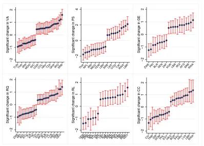
With regards to the time series dimension, the uncertainty around the WGI estimates
implies that changes in their values over time cannot be considered statistically
signifi-cant for a large number of countries. Figure 2 report the countries for which we cannot
reject the absence of change between 1996 and 2010. The mean, lower bound, and
up-per bound of these estimated changes correspond to the mean, 5th percentile and 95th
percentile of 200 imputed changes. It appears that few countries have experienced
sta-tistically significant changes in governance over a period of fourteen years. Stasta-tistically
frequent in RL (about 14% of the countries). Finally, it is interesting to note that some
countries, like Rwanda (RWA) or Zimbabwe (ZWE) have experienced changes is several
governance dimensions. It is of course possible that these various changes are driven by
a common latent governance factor.12
−2
−1
0
1
2
Significant change in VA
TUNTHA IRNMDG NICUGACOLHRV TZAGHA IRQSRB
−2
0
2
4
Significant change in PS
THA NPL IRNMDGYEMLBNSRB LKACOG TJKRWALBR
−2
−1
0
1
2
Significant change in GE
ZWE PRI BLR SEN ZAFKOR LBR IRQ AFG SRBRWA
−2
−1
0
1
2
Significant change in RQ
ZWENPLBOLECUITAKGZCIVSVKMOZALBCOLLVAHRVSRBGEO
−2
−1
0
1
2
Significant change in RL
VENARGZWEERIBOLECUIDNROULBYALBHRVSRBAZEBGRSLELBRIRQRWAGEO
−2
−1
0
1
2
Significant change in CC
[image:14.595.111.509.199.485.2]CIVTKM ISRDOMPHLEGYHKGBGRSAUHRVLVALBRRWA
Figure 2: Estimates of change in governance for countries with significant change (inter-val from 5thto 95thpercentile in red)
We ought to stress that the standard errors provided by the WGI project reflect the
assumption that errors are not correlated across sources. If this assumption is wrong, one
implication is that the standard errors of the WGI estimates are understated.13 Figure
3 illustrates the impact that larger standard errors can have. The number of countries
for which changes in GE have been statistically significant over the period 1996-2010
drastically falls when uncertainty around the WGI estimates increases.
12A list of the country ISO codes that we use can be found here http://en.wikipedia.org/wiki/ISO_3166-1
13Intuitively that is because the informativeness of each data source is exaggerated with correlated errors.
−2
−1
0
1
2
Change in GE
ZWE PRIBLRSENZAFKORLBR IRQAFGSRBRWA
Standard errors provided
−2
−1
0
1
2
ZWE CIV PRITCDSEN IRQ SLV ETHSRBGEORWA
Standard errors provided *1.25
−2
−1
0
1
2
ZWE CIV RWA
[image:15.595.103.526.98.270.2]Standard errors provided *1.50
Figure 3: Impact of larger standard errors on the number of countries which have experi-enced a significant change in governance (interval from 5thto 95thpercentile in red)
Overall, a comparison of the confidence intervals depicted in Figure 1 and Figure 2
suggests that taking into account the uncertainty of the WGI estimates is likely to have
more impact on research exploiting the time-series variation in the WGI than on studies
exploiting their cross-sectional dimension. The three applications that we now present
use a variety of estimators to assess this issue: pooled, fixed effects, cross-sectional
in-strumental variables.
3.2
Application 1: Capital flows
3.2.1 Introduction
In a recent paper, Binici, Hutchison, and Schindler (2010) (henceforth BHS) primarily
in-vestigate the impact of inward and outward capital controls on debt and equity flows.
Nev-ertheless, among their key results, they find that higher institutional quality, as measured
by the average of the six WGI, increases inflows and decreases outflows for both debt
and equity. These results echo those of Daude and Stein (2007), Alfaro, Kalemli-Ozcan,
and Volosovych (2008), Faria and Mauro (2009) or Azémar and Desbordes (2013). They
have been frequently interpreted as providing a partial answer to the Lucas Paradox. Poor
their poor governance.
3.2.2 Data and econometric methods
In BHS, the dependent variable is the log of financial flows per capita; these financial flows
can be equity inflows, debt inflows, equity outflows or debt outflows. The explanatory
variables arede jurecapital account restrictions, various control variables and the average
of the six WGI.14Like them, we omit oil-exporting countries and keep our sample constant
across regressions. Overall, our sample covers 71 countries over the period 1998-2005.15
We re-examine the regressions of Table 3 of their paper.
BHS estimate their log-linearised model using a fixed effects OLS estimator and a
sample devoid of zero values. In a first stage, we do the same. In a second stage, we
use a Poisson fixed effects estimator,16 and we model the conditional mean of financial
flows instead of modelling the conditional mean of the log of these flows. This gives us the
opportunity to show that our multiple imputation approach can be employed with a variety
of estimators while investigating whether BHS’s results are robust to the inclusion of zeros
values in their sample (a truncation issue) and/or the likely presence of heteroskedasticity.
In both cases, the elasticity of capital flows to population is restricted to unity. Standard
errors are clustered at the country level.
14They use the average of the percentile rank of the six indicators. We use the average of the WGI
estimates. In that way, we retain cardinal information which would be lost with ranking. Furthermore, we avoid the possibility of a fall in the percentile rank despite better governance. Finally, percentile ranking is sensitive to the introduction of new countries. Nevertheless, in unreported regressions, we find that our key results are unchanged when we use the average of the percentile rank of the six indicators as measure of institutional quality.
15They report having data over the period 1995-2005. However, data on debt inflow/outflow restrictions
are only available from 1997. In addition, the number of observations that they report (727) seem very high given that values for the governance variables are missing for the years 1995, 1997, 1999, 2001. Assuming no other missing data, the number of observations in their sample ought to have been 518 (74 [countries]× 7 [years])).
16This estimator is robust to distributional misspecification and therefore, as long as the conditional
3.2.3 Empirical results
Our results are presented in Table 1. In the upper panel, columns (1)-(4) are regressions
the most comparable to those carried out by BHS in Table 3 of their paper, while columns
(5)-(8) report the estimates applying the Poisson fixed effects estimator. The multiple
imputation results are provided in the lower panel of Table 1 in columns (1’)-(8’).
The results of columns (1-4) mirror, at least in qualitative terms, BHS’s key findings.
Like them, we find that restrictions on capital outflows appear to be much more effective
than restrictions on capital inflows and that higher institutional quality tends to encourage
capital inflows and discourage capital inflows.17 However, columns (1’)-(4’) present a
very different picture once we take into account the uncertainty with which the governance
variables are measured. In all columns, the estimated coefficient on institutional quality
becomes much smaller and is no longer statistically significant at conventional levels.
Furthermore, the estimated coefficients on some of the non-imputed variables also lose
statistical significance.
Columns (5)-(8) show that the initial results of BHS are not robust to the use of the
Poisson fixed effects estimator. Even when we do not do multiple imputation, we no
longer find that capital controls and institutional quality influence capital flows.18 The use
of multiple imputation does not change these conclusions and, as in columns (1’)-(4’),
lead to a strong attenuation of the estimated coefficient on the governance variable.
Overall, we find that BHS’s key findings are not robust to accounting explicitly for
the uncertainty of the WGI. Our multiple imputation approach leads to a very large fall
in the magnitude of the estimated coefficient on the governance variable, rendering it
sta-tistically insignificant. The reliance of this study on short-run changes to identify the
effects of governance on capital flows may explain this result. Furthermore, even
with-17Results for the other control variables are also very similar across the two studies.
18Note that inclusion of the zero values increases sample size by about one-third. However, differences
Table 1: Capital flows and governance
Debt securities FDI+portfolio equity Debt securities FDI+portfolio equity
Inflow Outflow Inflow Outflow Inflow Outflow Inflow Outflow ln(flow/population); Within estimator flow with offset ln(population); Poisson FE estimator (1) (2) (3) (4) (5) (6) (7) (8) Average six WGI 1.190* -0.483 1.924*** -1.757*** 0.468 -0.533 0.700 -1.835
(0.660) (0.606) (0.714) (0.625) (0.785) (0.819) (0.572) (1.202) ln(GDP per cap) 4.796*** 3.395*** 4.184*** 4.951*** 7.406*** 3.239*** 5.299*** 2.587***
(1.302) (0.928) (1.487) (1.383) (1.852) (1.164) (1.295) (0.906) Capital in/out-flow control -0.354 -0.473* -0.361 -0.644* 0.340 -0.861* -0.331 0.104
(0.344) (0.253) (0.492) (0.357) (0.524) (0.492) (0.432) (0.604) Private credit/GDP 0.131 1.123 0.198 0.836* 0.263 -0.147 -0.674 0.712* (0.707) (0.682) (0.593) (0.487) (0.504) (0.502) (0.642) (0.387) STMK CAP/GDP -0.439 -0.151 0.137 0.615** -0.816* -1.098*** -0.178 0.259
(0.419) (0.395) (0.447) (0.266) (0.427) (0.410) (0.324) (0.249) (Fuel,Metals,Ore)/Exports -2.831 2.941 3.146 -2.190 -7.801** 5.714 2.235 -2.040 (2.891) (2.055) (3.451) (2.360) (3.053) (3.481) (3.821) (1.448) Trade openness -1.700** -0.806 -0.964 -0.101 -2.703*** -1.086 -0.943* 0.130
(0.806) (0.564) (0.782) (0.749) (0.944) (0.701) (0.527) (0.635)
Taking into account WGI uncertainty
(1’) (2’) (3’) (4’) (5’) (6’) (7’) (8’) Average six WGI 0.203 -0.109 0.366 -0.365 0.092 -0.024 0.082 -0.194
(0.410) (0.335) (0.428) (0.387) (0.417) (0.435) (0.353) (0.430) ln(GDP per cap) 5.026*** 3.317*** 4.607*** 4.555*** 7.264*** 3.290*** 5.211*** 2.968** (1.303) (0.942) (1.506) (1.404) (1.732) (1.183) (1.256) (1.295) Capital in/out-flow control -0.468 -0.435 -0.394 -0.645* 0.336 -0.812 -0.376 0.273
(0.348) (0.263) (0.538) (0.356) (0.510) (0.500) (0.460) (0.570) Private credit/GDP 0.089 1.142* 0.121 0.909* 0.214 -0.072 -0.740 0.957** (0.726) (0.676) (0.604) (0.495) (0.501) (0.501) (0.665) (0.405) STMK CAP/GDP -0.329 -0.193 0.313 0.455 -0.727* -1.217*** -0.075 0.013
(0.413) (0.404) (0.462) (0.283) (0.376) (0.407) (0.308) (0.424) (Fuel,Metals,Ore)/Exports -3.408 3.116 2.204 -1.340 -8.101*** 6.222* 1.784 -0.778 (2.940) (2.070) (3.806) (2.890) (2.991) (3.495) (3.596) (2.260) Trade openness -1.705** -0.807 -0.976 -0.083 -2.735*** -1.022 -0.867 -0.162 (0.850) (0.559) (0.842) (0.745) (0.985) (0.639) (0.551) (0.418) Observations 297 297 297 297 400 400 400 400
out applying multiple imputation, BHS’s results vanish when we use an alternative fixed
effects estimator, which allows for both the dependent variable to be equal to zero and
heteroskedasticity.
3.3
Application 2: International trade
3.3.1 Introduction
Berden, Bergstrand, and Etten (2014) (henceforth BBE) investigate the impact of
gover-nance on international trade.19 They estimate gravity equations in which they include, on
the destination (importing) side, the six WGI separately in order to isolate their respective
impacts. They find that VA and PS both reduce trade overall, whereas RQ increases it.
Other WGI (GE, RL, CC) are not statistically significant. They conclude that democracy
reduces trade when its main effect is to give more voice to those likely to be affected
by international competition, e.g. unskilled workers. This result contrasts with previous
literature, which has typically found a positive relationship between democracy and trade
openness (Milner and Mukherjee, 2009). BBE argue that is because earlier works did not
specifically focus on the pluralism dimension of democracy.
3.3.2 Data and econometric methods
In BBE, the dependent variable corresponds to bilateral exports. The explanatory
vari-ables are those which are traditionally found in gravity-type equations (GDP, GDP per
capita, bilateral distance, contiguity, common language, colonial history, proxies for
mul-tilateral resistance) and the six WGI.20They use trade data for the period 1997-2004. We
simply use all the trade data available in our data source for the same time period. Our
dataset includes bilateral trade between 180 countries across five years (1998, 2000, 2002,
2003, 2004).
19They also look at the impact of governance on foreign direct investment.
20As in the previous application, the authors use their percentile rank while we use their conditional
In a first stage, we re-examine one of the main regressions in their paper which is
presented in column (6) of their Table 8. Like them, our estimator is the Poisson
quasi-maximum likelihood (QML) estimator and standard errors are clustered at the importing
country level. In a second stage, we investigate the impact of exporting countries’
gover-nance on bilateral trade. We also examine whether BBE’s findings are robust to the
inclu-sion of country-pair specific fixed effects, i.e. to the potential omisinclu-sion of time-invariant
relevant variables which are correlated with the WGI. This is a standard specification test
in studies involving panel data. Indeed Wooldridge (2009) argues that “in many
appli-cations, the whole reason for using panel data is to allow the unobserved effect to be
correlated with the explanatory variables” (p. 490).
3.3.3 Empirical results
Our results are presented in Table 2. Column (1) is the regression the most comparable to
that estimated by BBE in column (6) of Table 8 in their paper. In column (2), we include
the WGI on the exporting side. Columns (1’)-(2’) provide the multiple imputation results.
In columns (3)-(4’), we repeat the same empirical exercise, but using here a fixed effects
Poisson estimator instead of a Poisson QML estimator.
The results of column (1) echo the key finding of BBE: destination VA has a strong,
negative, and statistically significant impact on trade.21 On the other hand, we fail to find
a statistically significant relationship between trade and destination PS or destination RQ.
Column (2) shows that introducing the WGI on the exporting side does not change these
results and, overall, imports and exports are influenced in the same way by the various
governance dimensions. Columns (1’) and (2’) show that, relative to what happened in our
previous application, our multiple imputation approach has a much more nuanced
influ-ence on the non-imputed results here. The estimated coefficients on VA/GE/RQ/RL/CC,
on both exporting and importing sides, are very similar to those found in column (1) and
(2). On the other hand, in the case of destination PS, its estimated coefficient becomes
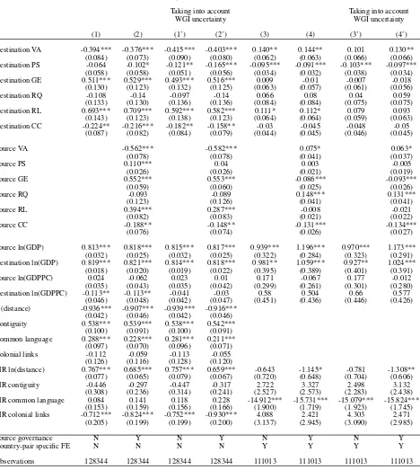
Table 2: Bilateral trade flows and governance
Bilateral trade flows
Pooled Poisson QMLE Fixed effects (FE) Poisson estimator Taking into account Taking into account
WGI uncertainty WGI uncertainty (1) (2) (1’) (2’) (3) (4) (3’) (4’) Destination VA -0.394*** -0.376*** -0.415*** -0.403*** 0.140** 0.144** 0.101 0.130**
(0.084) (0.073) (0.090) (0.080) (0.062) (0.063) (0.066) (0.066) Destination PS -0.064 -0.102* -0.121** -0.165*** -0.095*** -0.091*** -0.103*** -0.097***
(0.058) (0.058) (0.051) (0.056) (0.034) (0.032) (0.038) (0.034) Destination GE 0.511*** 0.529*** 0.493*** 0.516*** 0.009 -0.01 -0.007 -0.018 (0.130) (0.123) (0.132) (0.125) (0.063) (0.057) (0.061) (0.056) Destination RQ -0.108 -0.14 -0.097 -0.14 0.066 0.08 0.04 0.059
(0.133) (0.130) (0.136) (0.136) (0.084) (0.084) (0.075) (0.075) Destination RL 0.693*** 0.709*** 0.592*** 0.582*** 0.111* 0.112* 0.079 0.093
(0.143) (0.123) (0.138) (0.123) (0.064) (0.064) (0.059) (0.063) Destination CC -0.224** -0.216*** -0.182** -0.158** -0.03 -0.045 -0.048 -0.05
(0.087) (0.082) (0.084) (0.079) (0.044) (0.045) (0.046) (0.045) Source VA -0.562*** -0.582*** 0.075* 0.063* (0.078) (0.078) (0.041) (0.037)
Source PS 0.110*** 0.04 0.003 -0.005
(0.026) (0.026) (0.021) (0.019) Source GE 0.552*** 0.553*** -0.086*** -0.093***
(0.059) (0.060) (0.025) (0.026)
Source RQ -0.093 -0.089 0.148*** 0.131***
(0.123) (0.126) (0.041) (0.041) Source RL 0.394*** 0.287*** -0.008 -0.021 (0.082) (0.083) (0.021) (0.022) Source CC -0.188** -0.148** -0.131*** -0.134***
(0.076) (0.074) (0.026) (0.027) Source ln(GDP) 0.813*** 0.818*** 0.815*** 0.817*** 0.939*** 1.196*** 0.970*** 1.173***
(0.032) (0.025) (0.032) (0.025) (0.322) (0.284) (0.323) (0.291) Destination ln(GDP) 0.819*** 0.821*** 0.814*** 0.818*** 0.981** 1.059*** 0.927** 1.024***
(0.018) (0.020) (0.019) (0.022) (0.395) (0.389) (0.401) (0.391) Source ln(GDPPC) 0.024 -0.062 0.023 0.01 0.171 -0.067 0.177 -0.012 (0.035) (0.043) (0.035) (0.042) (0.299) (0.261) (0.301) (0.280) Destination ln(GDPPC) -0.113** -0.113** -0.041 -0.03 0.58 0.504 0.66 0.577
(0.046) (0.048) (0.042) (0.047) (0.451) (0.436) (0.446) (0.426) ln(distance) -0.936*** -0.907*** -0.939*** -0.916***
(0.042) (0.046) (0.042) (0.046) Contiguity 0.538*** 0.539*** 0.538*** 0.542***
(0.100) (0.091) (0.100) (0.091) Common language 0.288*** 0.228*** 0.281*** 0.211***
(0.097) (0.070) (0.096) (0.071) Colonial links -0.112 -0.059 -0.113 -0.055 (0.126) (0.116) (0.128) (0.120)
MR ln(distance) 0.767*** 0.685*** 0.757*** 0.659*** -0.643 -1.145* -0.781 -1.308** (0.077) (0.065) (0.079) (0.067) (0.720) (0.648) (0.704) (0.606) MR contiguity -0.446 -0.297 -0.447 -0.317 2.722 3.327 2.498 3.132
(0.308) (0.236) (0.314) (0.241) (2.527) (2.573) (2.283) (2.438) MR common language 0.084 0.141 0.118 0.228 -14.912*** -15.731*** -15.079*** -15.824***
(0.153) (0.159) (0.156) (0.166) (1.900) (1.719) (1.923) (1.745) MR colonial links -0.712*** -0.824*** -0.752*** -0.930*** 4.088 2.421 4.303 2.471
(0.205) (0.199) (0.199) (0.200) (3.137) (2.945) (3.090) (2.985)
Source governance N Y N Y N Y N Y
Country-pair specific FE N N N N Y Y Y Y
Observations 128344 128344 128344 128344 111013 111013 111013 111013
larger and now statistically significant at the 5% level whereas the opposite is true for the
estimated coefficient on source PS. Interestingly, the estimated coefficient on importing
country’s GDP per capita becomes much smaller and loses statistical significance with
multiple imputation.
In columns (3’)-(4’), we introduce country-pair specific fixed effects, controlling in
that way for unobserved time-invariant factors which may be correlated with the WGI.22
The inclusion of these fixed effects has a dramatic consequence for BBE’s key result that
higher destination VA tends to reduce trade. We now find that the VA variable has a
positive and statistically significant coefficient on both the importing and exporting sides.
That is, we are now finding that countries with stronger VA trade more with each other.
This holds true regardless of whether we use multiple imputation or not. This reversal of
results suggests that the negative effect of destination VA on trade is driven by an omitted
variable.23
Overall, we find that the key findings of BBE are robust to accounting explicitly for
the uncertainty of the VA indicator. This is possibly due to the use of a pooled estimator,
which exploits both the cross-sectional and time-series dimensions of VA. It is worth
not-ing that our conclusion would have been different if BBE had focused on destination PS;
with multiple imputation, its estimated coefficient becomes much larger and statistically
significant at conventional levels. In addition, BBE’s results are reversed when we include
country-pair specific fixed effects, suggesting the presence of an omitted variable bias.
22Similar results are found when we omit the proxies for multilateral resistance.
23It is also possible that democratisation has a short-term positive effect on trade, which vanishes and even
3.4
Application 3: Income levels around the world
3.4.1 Introduction
In a seminal paper, Rodrik, Subramanian, and Trebbi (2004) (henceforth RST) investigate
the independent contributions of geography, international integration, and institutions to
differences in income levels. To avoid any endogeneity bias, they instrument integration
and institutions by the instruments suggested by Frankel and Romer (1999) (constructed
“natural” openness) and Acemoglu, Johnson, and Robinson (2001) (settler mortality).
They find that“the quality of institutions ‘trumps’ everything else”(p.131).
3.4.2 Data and econometric methods
RST regress the log of GDP per capita in 1995 ($ PPP) on the absolute latitude of a country
(geography), the ratio of nominal trade to nominal GDP (integration), and the WGI Rule
of Law for the year 2001 (Institutions). We use the data made available by Dani Rodrik
on his website, except for the Rule of Law indicator; the standard errors of the estimated
values of this governance dimension are not provided. Our estimates for Rule of Law, and
their standard errors, correspond to the year 2000. The sample includes 79 countries from
around the world.
We first re-visit their preferred regression, which is presented in column (6) of their
Table 1. Then, we examine whether their results are robust to the presence of influential
observations in their sample or regional effects, as advocated by Temple (1999). We
use a two-stage least square estimator. For each regression, we report the Angrist and
Pischke (2009) multivariate first-stageF-statistic, which accounts for the presence of two
endogenous regressors, for the instrument ln(settler mortality).24
24Instruments are usually said to be strong (relevant) when the value of theF-statistic is around 10 or
3.4.3 Empirical results
Our results are presented in Table 3. The second-stage results are in the upper panel
and the first-stage results are in the lower panel. Column (1) is the regression the most
comparable to that estimated by RST in column (6) of their Table 1. In columns (2) and (3)
we include various dummies to control for influential observations and regional effects.
Columns (1’)-(3’) provide the multiple imputation results.
The results of column (1) are very similar to those of RST. Like them, we find that
in-stitutions trump geography and trade openness. The Angrist-PischkeF-statistic suggests
that the log of settler mortality is a slightly weak but nevertheless relevant instrument.
Column (1’) shows that the main impact of using multiple imputation is a lower partial
correlation between institutions and ln(settler mortality). This is reflected in a fall in the
value of the Angrist-PischkeF-statistic.
Worries have been expressed in the literature (e.g. Dollar and Kraay (2003),
Ro-drik, Subramanian, and Trebbi (2004), Albouy (2012)) about the influence of some
ob-servations on instrumental variables results involving the use of Acemoglu, Johnson, and
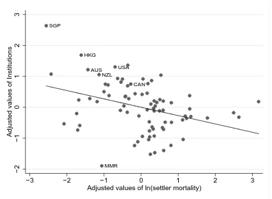
Robinson (2001)’s instrument. Figure 4, which is based on column (1) and depicts the
partial relationship between institutions and ln(settler mortality), highlights potential
out-liers. These observations correspond to East-Asia growth miracle countries (Hong-Kong
and Singapore), neo-European countries (Australia, Canada, New Zealand, United States)
and Myanmar.
To control for the influence of these observations, we add two dummies in columns
(2)-(2’): a Myanmar dummy variable and a “successful countries” dummy variable, which
takes the value of one if the country is either a East-Asia growth miracle country or a
neo-European country. The coefficient on institutions remains positive , statistically
signifi-cant, and is now larger than in column (1). It is however much less precisely estimated, as
the presence of the two dummy variables reduces the relevance of the instrument ln(settler
Table 3: Long-run economic development and governance
ln(GDP per capita in 1995)
IV estimation Taking into account WGI uncertainty
(1) (2) (3) (1’) (2’) (3’)
Institutions 1.853*** 2.783*** 6.159 1.887*** 2.981 15.495
(0.464) (0.985) (11.638) (0.609) (1.934) (14664)
Geography -0.012 -0.016 -0.061 -0.012 -0.018 -0.220
(0.019) (0.025) (0.170) (0.025) (0.045) (266)
Integration -0.053 -0.304 -1.063 -0.064 -0.362 -3.846
(0.243) (0.423) (2.878) (0.333) (0.732) (4140)
Successful countries -3.113* -9.818 -3.453 -27.063
(1.684) (21.714) (3.262) (29164)
Myanmar 4.485*** 9.123 4.866 23.784
(1.596) (17.199) (3.182) (20181)
Africa 0.446 1.255
(2.336) (650)
Latin America -2.700 -8.038
(6.313) (9648)
Institutions: first-stage
OLS estimation Taking into account WGI uncertainty
(1) (2) (3) (1’) (2’) (3’)
ln(settler mortality) -0.270*** -0.158** -0.048 -0.269** -0.157* -0.046
(0.098) (0.067) (0.086) (0.106) (0.080) (0.099)
Geography 0.020** 0.012 0.011 0.019* 0.011 0.010
(0.010) (0.008) (0.008) (0.011) (0.009) (0.009)
Constructed Openness 0.108 0.134 0.138 0.109 0.135 0.139
(0.117) (0.103) (0.095) (0.130) (0.118) (0.111)
Successful countries 1.549*** 1.901*** 1.556*** 1.911***
(0.232) (0.240) (0.285) (0.300)
Myanmar -1.952*** -1.726*** -1.974*** -1.746***
(0.127) (0.181) (0.309) (0.348)
Africa -0.208 -0.209
(0.261) (0.295)
Latin America 0.477** 0.482*
(0.218) (0.250)
Angrist-PischkeF-statistic Institutions 6.62 3.95 0.18 5.51 2.69 0.11
Observations 79 79 79 79 79 79
SGP
HKG
AUS NZL
MMR USA
CAN
−2
−1
0
1
2
3
Adjusted values of Institutions
−3 −2 −1 0 1 2 3
[image:26.595.111.508.95.386.2]Adjusted values of ln(settler mortality)
Figure 4: Partial relationship between institutions and ln(settler mortality)
magnified by the use of multiple imputation. In column (2’), the Angrist-Pischke F
-statistic is smaller than in column (2) and the standard error of the estimated coefficient
on institutions is so large that we cannot reject anymore the absence of a statistically
significant effect of institutions on income levels.
In columns (3)-(3’), we add regional dummy variables for Latin America and Africa.
With the inclusion of these regional effects, the instrument ln(settler mortality) becomes
completely irrelevant and the use of this now weak instrument leads to a very large
stan-dard error of the estimated coefficient on institutions. This is especially true in the multiple
imputation regression, where the values of the standard errors are 3-5 digits numbers.25
Overall, we find that the widely disseminated findings of RST do not hold once we
account simultaneously for the uncertainty around the WGI estimates and the presence
25These abnormally large standard errors are due to a small fraction of imputations in which there is no
of influential observations/regions in their sample. The use of multiple imputation plays
a large role in the invalidation of RST’s results, by weakening the partial correlation
be-tween institutions and Acemoglu, Johnson, and Robinson (2001)’s instrument. Hence,
even when the WGI are used, in a cross-sectional context, as dependent variable,
uncer-tainty around their estimates still matter.
4
Conclusions
Our various applications have highlighted that the estimated effects of governance on
various aspects of economic development are extremely sensitive to uncertainty in both
the WGI estimates and model specification. Accounting for the uncertainty around the
WGI estimates through multiple imputation frequently had a large influence on the size
and statistical effects of the different governance dimensions, and occasionally, of other
explanatory variables. Furthermore, none of the results of the studies that we revisited
survived standard changes in model specification.
This paper shows that the empirical effects of governance can be elusive. Identification
of its impact is constantly threatened by the possibilities of measurement error, omitted
variable bias, or reverse causality. The efforts of the researcher are not helped by the
difficulties of finding a valid instrument, even in a cross-sectional context. Hence, in
many cases, the adequate econometric treatment of the uncertainty associated with the
WGI coupled with careful model specification remain the most reasonable approach to
References
Acemoglu, D., S. Johnson, and J. A. Robinson, 2001, “The Colonial Origins of
Compar-ative Development: An Empirical Investigation,” American Economic Review, 91(5),
1369–1401.
Albouy, D. Y., 2012, “The colonial Origins of Comparative Development: An Empirical
Investigation: Comment,”American Economic Review, 102(6), 3059–3076.
Alfaro, L., S. Kalemli-Ozcan, and V. Volosovych, 2008, “Why Doesn’t Capital Flow
from Rich to Poor Countries? An Empirical Investigation,” Review of Economics and
Statistics, 90(2), 347–368.
Angrist, J. D., and J.-S. Pischke, 2009,Mostly Harmless Econometrics: An Empiricist’s
Companion. Princeton: Princeton University Press.
Arndt, C., and C. Oman, 2006,Uses and Abuses of Governance Indicators. Paris: OECD.
Azémar, C., J. Darby, R. Desbordes, and I. Wooton, 2012, “Market Familiarity and the
Location of South and North MNEs,”Economics & Politics, 24(3), 307–345.
Azémar, C., and R. Desbordes, 2009, “Public Governance, Health and Foreign Direct
Investment in Sub-Saharan Africa,”Journal of African Economies, 18(4), 667–709.
, 2013, “Has the Lucas Paradox Been Fully Explained?,” Economics Letters,
121(2), 183–187.
Baier, S. L., and J. H. Bergstrand, 2009, “Bonus Vetus OLS: A Simple Method For
Ap-proximating International Trade-Cost Effects Using the Gravity Equation,” Journal of
International Economics, 77(1), 77–85.
Beck, T., A. Demirguc-Kunt, and R. Levine, 2009, “Financial Institutions and Markets
Across Countries and Over Time - Data and Analysis,” Policy Research Working Paper
Berden, K., J. H. Bergstrand, and E. Etten, 2014, “Governance and Globalisation,” The
World Economy, 37(3), 353–386.
Binici, M., M. Hutchison, and M. Schindler, 2010, “Controlling Capital? Legal
Restric-tions and the Asset Composition of International Financial Flows,”Journal of
Interna-tional Money and Finance, 29(4), 666–684.
Blackwell, M., J. Honaker, and G. King, 2012, “Multiple Overimputation: A Unified
Approach to Measurement Error and Missing Data,” mimeo.
Brownstone, D., and R. G. Valletta, 1996, “Modeling Earnings Measurement Error: A
Multiple Imputation Approach,”Review of Economics and Statistics, pp. 705–717.
Carroll, R. J., D. Ruppert, L. A. S. Stefansky, and C. M. Crainiceanu, 2006,Measurement
Error in Nonlinear Models. Boca Raton: Chapman & Hall/CRC.
Daude, C., and E. Stein, 2007, “The Quality of Institutions and Foreign Direct
Invest-ment,”Economics and Politics, 19(3), 317–344.
Dietrich, S., 2013, “Bypass or Engage? Explaining Donor Delivery Tactics in Foreign
Aid Allocation,”International Studies Quaterly, 54(4), 698–712.
Dollar, D., and A. Kraay, 2002, “Growth is Good for the Poor,” Journal of economic
growth, 7(3), 195–225.
, 2003, “Institutions, Trade, and Growth,”Journal of Monetary Economics, 50(1),
133–162.
Faria, A., and P. Mauro, 2009, “Institutions and the External Capital Structure of
Coun-tries,”Journal of International Money and Finance, 28(3), 367–391.
Frankel, J. A., and D. Romer, 1999, “Does Trade Cause Growth?,”American Economic
Head, K., T. Mayer, and J. Ries, 2010, “The Erosion of Colonial Trade Linkages After
Independence,”Journal of International Economics, 81(1), 1–14.
Høyland, B., K. Moene, and F. Willumsen, 2012, “The Tyranny of International Index
Rankings,”Journal of Development Economics, 97(1), 1–14.
Kaufmann, D., and A. Kraay, 2002, “Growth Without Governance,” Economia, 3(1),
169–229.
, 2008, “Governance Indicators: Where Are We, Where Should We Be Going?,”
The World Bank Research Observer, 23(1), 1–30.
Kaufmann, D., A. Kraay, and M. Mastruzzi, 2007, “The Worldwide Governance
Indica-tors Project: Answering the Critics,” World Bank Policy Research Department Working
Paper, No. 4149.
, 2009, “Governance Matters VIII: Aggregate and Individual Indicators,
1996-2008,” World Bank Policy Research Paper, No. 4978.
, 2011, “The Worldwide Governance Indicators: Methodology and Analytical
Issues,”Hague Journal on the Rule of Law, 3(02), 220–246.
Kaufmann, D., A. Kraay, and P. Zoido-Lobaton, 1999, “Aggregating Governance
Indica-tors,” World Bank Working Paper, No. 2195.
Koop, G., 2003,Bayesian Econometrics. John Wiley and Sons.
Kraay, A., 2006, “When is Growth Pro-Poor? Evidence From a Panel of Countries,”
Journal of development economics, 80(1), 198–227.
Lane, P. R., and G. M. Milesi-Ferretti, 2007, “The External Wealth of Nations Mark II:
Revised and Extended Estimates of Foreign Assets and Liabilities, 1970-2004,”Journal
Méon, P.-G., and K. Sekkat, 2008, “Institutional quality and trade: which institutions?
Which trade?,”Economic Inquiry, 46(2), 227–240.
Milner, H. V., and B. Mukherjee, 2009, “Democratization and Economic Globalization,”
Annual Review of Political Science, 12, 163–181.
Pemstein, D., S. A. Meserve, and J. Melton, 2010, “Democratic Compromise: A Latent
Variable Analysis of Ten Measures of Regime Type,” Political Analysis, 18(4), 426–
449.
Rodrik, D., A. Subramanian, and A. Trebbi, 2004, “Institutions Rule: The Primacy of
Institutions Over Geography and Integration in Economic Development,” Journal of
Economic Growth, 9(2), 131–165.
Rubin, D. B., 1987, Multiple imputation for nonresponse in surveys. New York: John
Willey & Sons.
, 1996, “Multiple Imputation After 18+years,”Journal of the American Statisti-cal Association, 91(434), 473–489.
Santos Silva, J. M. C., and S. Tenreyro, 2006, “The Log of Gravity,”Review of Economics
and Statistics, 88(4), 641–658.
, 2011, “Further Simulation Evidence on the Performance of the Poisson
Pseudo-Maximum Likelihood Estimator,”Economics Letters, 112(2), 220–222.
Schafer, J. L., 1997,Analysis of Incomplete Multivariate Data. London: Chapman & Hall.
Staiger, D., and J. H. Stock, 1997, “Instrumental Variables Regression with Weak
Instru-ments,”Econometrica, 65(3), 557–586.
Standaert, S., forthcoming, “Divining the Level of Corruption: A Bayesian State-Space
Temple, J., 1999, “The New Growth Evidence,” Journal of Economic Literature, 37(1),
112–156.
Thomas, M. A., 2010, “What Do the Worldwide Governance Indicators Measure,”
Euro-pean Journal of Development Research, 22(1), 31–54.
Wei, S.-J., 2000, “How Taxing is Corruption on International Investors?,”Review of
Eco-nomics and Statistics, 82(1), 1–11.
Winkelmann, R., 2008, Econometric Analysis of Count Data. Berlin: Springer-Verlag
Berlin Heidelberg.
Winters, M. S., 2010, “Choosing to Target: What Types of Countries Get Different Types
of World Bank Projects,”World Politics, 62(3), 422–458.
Wooldridge, J. M., 2009,Introductory Econometrics. A Modern Approach. South-Western
College Publishing, international„ fourth edn.
Wooldridge, J. M., 2010, Econometric Analysis of Cross Section and Panel Data.