Artificial halo orbits for low-thrust propulsion spacecraft

(will be inserted by the editor)

Artificial Halo Orbits

for Low-Thrust Propulsion Spacecraft

Shahid Baig · Colin R. McInnes

Received: date / Accepted: date

Abstract We consider periodic halo orbits about artificial equilibrium points near to the Lagrange pointsL1andL2in the circular restricted three body problem, where the third body is a low-thrust propulsion spacecraft in the Sun-Earth system. Although such halo orbits about artificial equilibrium points can be generated using a solar sail, there are points insideL1and beyondL2where a solar sail cannot be placed, so low-thrust, such as solar electric propulsion, is the only option to generate artificial halo orbits around points inaccessible to a solar sail. Analytical and numerical halo orbits for such low-thrust propulsion systems are obtained by using the Lindstedt Poincar´e and differential corrector method respectively. Both the period and minimum amplitude of halo orbits about artificial equilibrium points insideL1 decreases with an increase in low-thrust acceleration. The halo orbits about artificial equilibrium points beyond L2 in contrast show an increase in period with an increase in low-thrust acceleration. However, the minimum amplitude first increases and then decreases after the thrust acceleration exceeds 0.415 mm/s2. Using a continuation method, we also find stable artificial halo orbits which can be sustained for long integration times and require a reasonably small low-thrust acceleration 0.0593 mm/s2.

Keywords Restricted three body problem· halo orbits·low-thrust propulsion· continuation method

1 Introduction

It is well-known that the circular restricted three-body problem (CRTBP) has five nat-ural equilibrium points. Three of them are on the axis joining the primaries (collinear

Shahid Baig, PhD Candidate

Department of Mechanical Engineering, University of Strathclyde, Glasgow, G1 1XJ, Scotland, UK.

E-mail: [email protected]

Colin R. McInnes, Professor

Department of Mechanical Engineering, University of Strathclyde, Glasgow, G1 1XJ, Scotland, UK.

Lagrange points) and two are on the vertices of equilateral triangles joining the pri-maries (equilateral Lagrange points). At Lagrange points the gravitational forces of the two primaries and the centrifugal force on a spacecraft in a rotating frame are balanced. Artificial equilibrium points (AEPs) other than Lagrange points can be generated by using a constant continuous acceleration from a low-thrust propulsion system such as a solar sail or solar electric propulsion system.

Around the collinear Lagrange points, ‘classical’ halo orbits have been extensively studied, for example Farquhar and Kamel [1], Breakwell and Brown [2], Richardson [3], Howell [4], Thurman and Worfolk [5]. Notably, Richardson [3, 6] used the method of Lindstedt Poincar´e to obtain a third-order analytical approximation of periodic halo orbits (unstable) in a simple, high-precision and straightforward manner. Stable halo orbits were found by Breakwell and Brown aroundL2in the Earth-Moon system [2], and later on by Howell [4] for a wide range of mass ratios around all three collinear Lagrange points in an extensive numerical study.

McInnes et al. [7] show continuous surfaces of AEPs can be generated in the CRTBP for a solar sail low-thrust propulsion system, but only in certain allowed regions. These AEPs are characterized by the sail lightness number and sail orientation. The linearized eigenvalue spectrum around AEPs contains at least one centre, so linear periodic orbits can be generated or the Lindstedt Poincar´e method can be applied. McInnes [8] and Baoyin and McInnes [9], describe halo orbits around AEPs on the line joining the two primaries in the solar-sail three body problem. However, McInnes [8] describes stable regions of halo orbits around unstable AEPs, when the amplitude of the halo orbit becomes large. Waters and McInnes [10] generate unstable ‘artificial’ halo orbits in the solar-sail CRTBP about AEPs, which are high above the ecliptic plane. However, for a solar sail, all of these ‘artificial’ halo orbits around AEPs, in and above the eclliptic plane, are in the allowed/accessible volume of space.

Morimoto et al. [11] find AEPs in the CRTBP for a solar electric or nuclear electric low-thrust propulsion system. These AEPs are characterized by the low-thrust accel-eration magnitude and thrust orientation. In particular, marginally stable regions in addition to unstable regions of AEPs are found that differ from the solar sail prob-lem which has only unstable regions of AEPs. Morimoto et al. [12] also find resonant periodic orbits with a constant, continuous acceleration at linear order around the marginally stable AEPs along the axis joining the primary bodies. In this paper, we extend this analysis of low-thrust periodic orbit at nonlinear order using the Lindstedt Poincar´e method about unstable AEPs on the line joining the two primaries. Further-more, we show the feasibility of halo orbits about AEPs where a solar sail cannot generate periodic orbits because of the requirement that the sail acceleration cannot be directed towards the Sun i.e., for AEPs inside L1 and beyond L2. The AEPs are chosen near to the natural Lagrange pointsL1 andL2to limit the power and thrust level from the low-thrust propulsion system. We also show the existence of stable halo orbits around unstable AEPs beyond L2, using the orbit half-period as a continua-tion parameter which results better convergence accuracy. Furthermore, spacecraft on stable orbits are found to require a reasonably small low-thrust acceleration pointing towards the Sun.

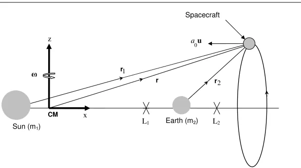
Sun (m1)

Earth (m2)

2

r

1

r

Spacecraft

0

au

x z

CM

r

L1 L2

Fig. 1 Definition of coordinate system and low-thrust spacecraft in a periodic halo orbit about

an artificial equilibrium point beyondL2.

2 Equations of Motion

The CRTBP is a dynamical model that describes the motion of an infinitesimal mass, a spacecraft under the gravitational influence of two massive bodies in circular motion. Consider a synodic coodinate frame i.e., co-rotating with the two primary massesm1 and m2 at constant angular velocityω with origin at their center of mass, as shown in Fig. 1. The x-axis points along the Sun-Earth line, the z-axis is the axis of rotation and the y-axis completes the right-handed coordinate system. The system is made nondimensional by taking the units of length, mass and time such that distance between the primaries, the product of gravitational constantGand sum of the masses of the primaries, and the period of the primaries is 1, 1 and 2π respectively. By defining µ= m2

m1+m2,m1is located at (−µ,0,0) andm2is located at (1−µ,0,0) with respect

to centre of mass. If we denote r= [x y z]T as the position vector of the low-thrust spacecraft relative to the centre of mass, then the position vector of the spacecraft with respect to the primariesm1andm2is given by

r1= [x+µ y z]T, r2= [x−(1−µ) y z]T

The nondimensional equation of motion of a low-thrust spacecraft in the rotating frame of reference is given by

¨

r+ 2ω_×r˙=∇V +a_0≡F ₍₁₎

whereV is the effective potential given by

V = µ

1−µ r1 +

µ r2

¶ +1

2(x 2_+y2₎

The vectora_{0is the acceleration due to the low-thrust propulsion system. At an}

equi-librium point ¨rand ˙rvanish, so an equilibrium point is a zero of F _i.e.,F_{(r0) =0.}

Thus, a nonequilibrium pointr0in the rotating frame is changed into an artificial equi-librium point with low-thrust acceleration vectora_{0satisfying the following condition}

where magnitude and direction of low-thrust acceleration is given by

a0=|∇V|

u=−_|∇∇V_V| (3)

Taking the dot product on both sides of Eq. (1) by ˙r=v_{, we get} v_.v_{˙+ 2}v_.(ω_×v₎₋v_.a₀₌v_{.∇V =} dr

dt. ∂V

∂r or

dh1₂vTv₋aT₀ri

dt =

dV dt

So we have the Jacobi constant for the low-thrust system given by

C(r,v_{) =}1

2v

T_v

−aT_{0r−V(r) (4)}

For the correct initial conditions, the spacecraft will move on a periodic orbit around an artificial equilibrium pointr0 with constant continuous acceleration a0 satisfying Eq. (3), and having the constant of motionC.

The classical case (with no propulsion) is Hamiltonian and time independent, so we have an energy integral of motion and this energy is defined by Eq. (4) witha₀₌

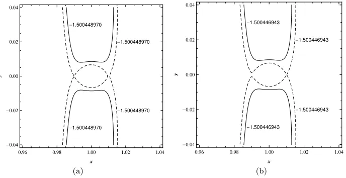
(0,0,0). At the Lagrange points L1 and L2 of the Sun-Earth system, the energies of the spacecraft at rest are−1.500448970 and−1.500446943 respectively.

-1.500448970

-1.500448970

-1.500448970

-1.500448970

0.96 0.98 1.00 1.02 1.04

-0.04 -0.02 0.00 0.02 0.04

x

y

-1.500446943

-1.500446943

-1.500446943

-1.500446943

0.96 0.98 1.00 1.02 1.04

-0.04 -0.02 0.00 0.02 0.04

x

y

(a) (b)

Fig. 2 Zero velocity curves in the Sun-Earth system for (a) energy values of theL1 and (b)

energy values of theL2point . For classical casea0= (0,0,0) (dashed contour lines) and for

low-thrust systema0= (0.0001,0,0) (solid contour lines)

Fig. 2 shows that classical case contours are closed for energy values atL1andL2 points (see dashed contour lines). However, in case of a low-thrust system for a_{0 =}

3 Linearized System

A linear system δ_X˙ _{= AδX in the vicinity of an equilibrium point r0 is obtained} from the nonlinear system Eq. (1) by using the transformation r = r0+δr, where

r0= (x0,0,0),δr= (δx, δy, δz)T andδX= (δr, δr˙)T. We assume the attitude of the low-thrust systemuis not perturbed so as to restrict the stability analysis in the sense of Lyapunov, furthermore a_{0 is fixed w.r.t. perturbation δri.e.,} ∂a0

∂r = 0. Then the Jacobian matrixAis given by

A= µ 0 I M Ω ¶ (5)

where I is the unity matrix. Moreover,

M =∂∇V ∂r ¯ ¯ ¯ ¯ ¯ r0 =   a0 0 0b0 0 0 e



, Ω= 

 0 2 0 −2 0 0 0 0 0





and

a= 2c+ 1, b= 1−c, e=−c

with

c(x0, µ) = µ

|x0+µ−1|3

+ 1−µ |x0+µ|3

>0

asµ >0 and 1−µ >0. In Eq. (5), thezequation is decoupled fromx,yequations for the AEPr0chosen on thex-axis (or in thex−yecliptic plane), so the out of ecliptic plane equation of motion is given by

δz¨+cδz= 0

which has a simple harmonic solution δz = Azsin(wzt+φz), where wz = √c. The characteristic polynomial for thex, ylinearized Eq. (5) rewritten in matrix form



  

δx˙ δy˙ δx¨ δy¨

    =    

0 0 1 0 0 0 0 1 a0 0 2 0 b−2 0

        δx δy δx˙ δy˙



  

(6)

is given by

p(λ) =λ4+ (2−c)λ2+ (1 +c−2c2)

By lettingα=λ2, then the roots ofp(α) = 0 are as follows

α1=c−2 +

√ 9c2_−8c

2 , α2=

c−2−√9c2_−8c

2 (7)

Letu_1+iw_{1be an eigenvector of the linearized Eq. (6) corresponding to eigenvalue}

iλ1and letv1andv2be the eigenvectors corresponding to eigenvalues +λr and−λr. Then, the generalized solution of Eq. (6) is [13]



  

δx δy δx˙ δy˙



  

= cos(wxyt)[Au1+Bw1] + sin(wxyt)[Bu1−Aw1]

+Ceλrt_v

1+De−λrtv2

(8)

where

u₁₌³_0,(a+wxy2 _),2w2_xy,0´T_,w₁₌³_{−2wxy,0,0, wxy(a+w}2_xy)´T

We setC= 0 andD= 0 to switch off the real modes to get bounded solutions forδx andδy. Finally, the three-dimensional bounded solution to the linear problem Eq. (5) can be written as

δx=−Axcos(wxyt+φxy), δy=kAxsin(wxyt+φxy),

δz=Azsin(wzt+φz)

(9)

with k = a+w

2 xy

2wxy . For the AEPs in this paper, the ratio of in-plane wxy and out of

frequencieswz is not a rational number, so a quasi-periodic Lissajous trajectory can be obtained as shown in Fig. 3.

-3000 3000

-10 000

10 000

∆xHkmL

∆

y

H

km

L

-10 000 10 000

-3000 3000

∆yHkmL

∆

z

H

km

L

-3000 3000

-3000 3000

∆xHkmL

∆

z

H

km

L

Fig. 3 Lissajous trajectory at AEPr0= [1.02 0 0]T (beyondL2) in the Sun-Earth system.

Ax =Az = 2.3396×10−5_{(3500 km) andφxy =φz = 0 are chosen for illustration purpose.} The AEP needsa0= (−0.0512,0,0).

4 Nonlinear Approximations

frequency of a periodic solution to the linear system. Therefore, the nonlinearity alters the frequency fromwxy towxyw. where

w= 1 +ǫw1+ǫ2w2+. . . (10)

This frequency correction allows us to remove secular terms through determination of widuring the development of the approximate periodic solution about AEPs.

A Taylor series expansion ofF _{to third-order [14] about AEPr0is found by making}

the transformationr→r0+δr, so we have the system of nonlinear equations

δ¨r+ 2ω_×δr˙=F_{(r0) +}

à δr.

· _∂

∂r ¸T!

∇V¯¯ ¯

r=r0

+ 1 2!

à δr.

·_∂

∂r ¸T!2

∇V¯¯ ¯

r=r0

+1 3!

à δr.

· ∂ ∂r

¸T!3 ∇V

¯ ¯ ¯

r=r0

+O(δr4)

where we have assumed that ∂a0

∂r ,

∂2_a 0

∂r2 etc., are all zero. So in component form the

equations of motion through third-order are given by

δx¨−2δy˙−(2c+ 1)δx= 3C³2δx2−δy2−δz2´

+ 4Dδx(2δx2−3δy2−3δz2) +O(δr4) δy¨+ 2δx˙+ (c−1)δy =−6Cδxδy

−3Dδy³4δx2−δy2−δz2´+O(δr4) δz¨+w2xyδz=−6Cδxδz

−3Dδz³4δx2−δy2−δz2´+O(δr4) +∆δz (11)

where C = Vxxx|r=_r0

12 and D =

Vxxxx|r=_r0

48 are evaluated at the AEPr0 = (x0,0,0). Note that the term∆=w2xy−c=w2xy−w2z=O(A2z) =O(ǫ2) is added in the right-hand-side of the z−equation to force a periodic orbit at linear order with frequency wxy (this periodic solution is given in Eq. (9) withwzreplaced by wxy and acts as a first approximation).

The following relations exist to switch off the secular term which appear as a result of successive approximation in the inhomogeneous part of the system of equations of orderO(ǫ2) andO(ǫ3).

w1= 0, w2=s1A2x+s2A2z

l1A2x+l2A2z+∆= 0, φz=φxy+nπ/2 n= 1,3

The expressions forsi, li are given in Ref. [5]. The closed orbit corresponding to these constraints is a halo orbit. Northern halo orbits, whose maximum out-of-plane compo-nent is above the ecliptic plane, are obtained corresponding to the solutionn= 1 and n= 3 about AEPs nearL1andL2 respectively. The period of the orbit can be found from the amplitude-frequency relation T = 2π/wxyw, where w = 1 +s1A2x+s2A2z. The minimum in-plane amplitudeAxmin=

p

complete third-order successive approximation solution of Eq. (11) using the Lindstedt Poincar´e method is given by [5]

δx(t) =−Axcosτ1+a21A2x+a22A2z+ (a23A2x+ζa24A2z) cos 2τ1 + (a31A3x+ζa32AxA2z) cos 3τ1

δy(t) =kAxsinτ1+ (b21A2x+ζb22Az2) sin 2τ1+ (b31A3x+ζb32AxA2z) sin 3τ1

+ (b33A3x+b34AxA2z+ζb35AxA2z) sinτ1

δz(t) = (−1)(n−1)/2Azcosτ1+ (−1)(n−1)/2d21AxAz(cos 2τ1−3)

+ (−1)(n−1)/2(d32AzA2x−d31A3z) cos 3τ1 (12)

whereζ= (−1)n andτ1=wxywt+φ. The constantssi, li, aij, bij anddij involveC,

D,k andwxy which in turn ultimately depend onr0 andµ. Note that the numerical values of these constants will be different from that given in [3, 5] due to the different scaled system chosen in nondimensionalization (see Sect. 2). In Eq. (12) the expres-sion for δy(t) also contains the third-order correction to the amplitude of sinτ1 by Thurman and Worfolk [5] in Richardson’s original solution [3]. This correction allows faster convergence of the differential corrector algorithm. Fig. 4 shows that the

magni-0.98 0.985 0.99 0.995

100 150 200 250 300 O rbi t P e ri od (da y s ) x0

0.98 0.985 0.99 0.995-0.4

-0.2 0 0.2 0.4 x -c om po ne n t of l ow -t hrus t a c c e le ra ti on (m m s

-2)

T

Required low-thrust acceleration

L1

1 1.005 1.01 1.015 1.02 1.025 1.03 1.035

0 100 200 300 400 O rbi t P e ri od (da y s ) x0

1 1.005 1.01 1.015 1.02 1.025 1.03 1.035-1

-0.5 0 0.5 1 x -c om po ne n t of l ow -t hrus t a c c e le ra ti on (m m s

-2)

T

Required low-thrust acceleration

L2

(a) (b)

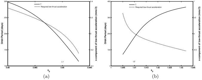
Fig. 4 Period of artificial halo orbit vs AEPs selected atx0near to (a)L1and (b)L2 points

in the Sun-Earth system. The dotted curve shows the low-thrust acceleration required atx0

to create AEPs.a0= 0 atL1andL2.

tude of the low-thrust accelerationa_{0is zero atL1andL2and increases to convert a}

nonequilibrium point atx0away fromL1andL2into an equilibrium point. Artificial L1 and L2 points are chosen that require a maximuma0≈0.05 (0.296 mms−2) and a0 ≈0.1 (0.593 mms−2), which corresponds to a thrust of 150 mN and 300 mN for a 500 kg spacecraft. For points insideL1and beyondL2, the direction ofa0is sunward, so these periodic artificial halo with a givenz−amplitude cannot be generated with a solar sail.

Fig. 4 also shows that period T = _(1+w2π

2)wxy of these artificial halo orbits follow

0.98 0.985 0.99 0.995 -0.04 -0.03 -0.02 -0.01 0 0.01 w 2 x0

0.98 0.985 0.99 0.9951

1.5 2 2.5 3 3.5 w x y w2 XYZ L1

1 1.005 1.01 1.015 1.02 1.025 1.03 1.035

-0.04 -0.02 0 0.02 w 2 x0

1 1.005 1.01 1.015 1.02 1.025 1.03 1.0350

2 4 6 w x y w2 X YZ L2 (a) (b)

Fig. 5 Zero and second order frequency adjustment (w2) vs AEPs selected atx0near to (a)

L1and (b)L2points in the Sun-Earth system.

0.980 0.985 0.99 0.995

2 4 6 8x 10

5 M ini m um x -a m pl it u de ( k m ) x0

0.98 0.985 0.99 0.995-0.4

-0.2 0 0.2 0.4 x -c om po ne n t of l ow -t hr us t a c c e le ra ti on (m m s

-2) A

xmin

Required low-thrust acceleration

L1

1 1.005 1.01 1.015 1.02 1.025 1.03 1.035

0 5 10x 10

5 M ini m um x -a m pl it u de ( k m ) x₀

1 1.005 1.01 1.015 1.02 1.025 1.03 1.035-1

0 1 x -c om po ne n t of l ow -t hrus t a c c e le ra ti on (m m s

-2) Axmin

Required low-thrust acceleration

L2

(a) (b)

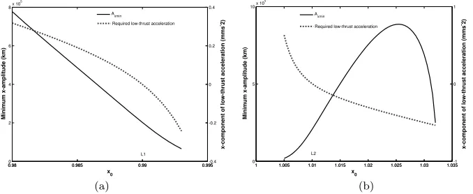
Fig. 6 The minimum x-amplitude to have artificial halo orbits vs AEPs selected atx0 near

to (a)L1and (b)L2points.

the period. Fig. 6 shows that the minimum amplitudeAxmin= q

|∆l1|beyond artificial L2 points first increases then decreases whena0exceeds≈0.07 (0.415 mms−2), as at this point the rate at which√∆decreases becomes more than the rate at which √1

|l1|

increases. Although in Figs. (4-5) Az is chosen 125000 km, the effect of Az on the second order frequency correctionw2, and so periodT is relatively small.

5 Differential Correction and Low-Thrust Halo orbits

We can use the initial guess from Lindstedt Poincar´e analysis to integrate the full nonlinear system of equations Eq. (1) along with the constant low-thrust acceleration

a₀=H0.01,0,0L a

0=H0.02,0,0L

0.986 0.988 0.990 0.992 x

-0.006

-0.004

-0.002

0.002 0.004 0.006 y

Classical halo

a

0=H-0.02,0,0L

a

0=H-0.01,0,0L

0.986 0.988 0.990 0.992 x

-0.002

-0.001

0.001 0.002 z

º

-0.006 -0.004 -0.002 0.002 0.004 0.006 y

-0.0005

0.0005 0.0010 z

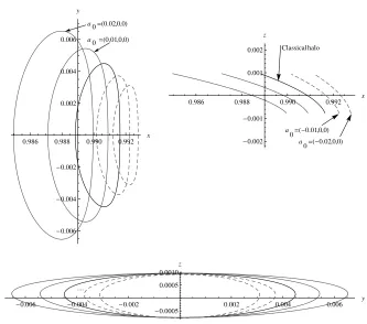
Fig. 7 Artificial halo orbits are shown in gray around artificial L1 points (n = 1) with

low thrust acceleration vectorsa0 = (±0.01,0,0) anda0 = (±0.02,0,0). The classical halo

orbit is also shown (3rd dark black orbit). All periodic orbits have same Az = 8.3557×

10−4_{(125000 km.)}

The nonlinear equations of motion Eq. (1) with constant a_{0 are symmetric}

un-der the transformation y → −y and t → −t, so this symmetry about the xz-plane suggests we need to determine periodic orbits for a half periodT_1/2 only. Let X0 = (x0,0, z0,0,y˙0,0) be initial data from Lindstedt Poincar´e, so the spacecraft leaves per-pendicularly from the y= 0 plane. On the first return to the y = 0 plane, its state is

X(T_1/2) = (˜x,0,z,˜x,˙˜ y,˙˜ z˙˜) so we have a periodic solution when ˙˜x= ˙˜z= 0.

a₀=H-0.01,0,0L

a₀=H-0.02,0,0L

1.010 1.012 1.014 x

-0.006

-0.004

-0.002 0.002 0.004 0.006 y

Classical halo a

0=H0.01,0,0L a

0=H0.02,0,0L

1.008 1.010 1.012 1.014 x

-0.001

0.001 0.002 z

-0.006 -0.004 -0.002 0.002 0.004 0.006 y

-0.0005

0.0005 z

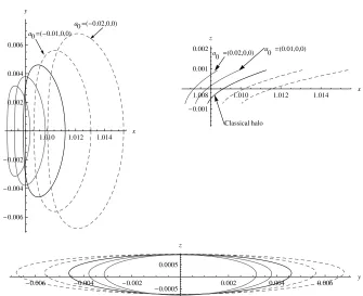
Fig. 8 Artificial halo orbits are shown in gray around artificial L2 points (n = 3) with

low thrust acceleration vectorsa0 = (±0.01,0,0) anda0 = (±0.02,0,0). The classical halo

orbit is also shown (3rd dark black orbit). All periodic orbits have same Az = 8.3557×

10−4_{(125000 km.)}

atT1/2+∆T1/2 by

∆X(T1/2+∆T1/2) =

∂X(T_1/2,X0)

∂X0 ∆

X0+ ˙X(T1/2)∆T1/2 (13)

The matrix ∂X

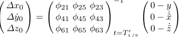
∂X0 = Φ is the state transition matrix evaluated along the reference

solution _X¯_{(t). To make ˙˜x = ˙˜z = 0 at y = 0, we vary x0, ˙y0, T}

1/2 iteratively by corrections ∆x0, ∆y˙0 and ∆T1/2 while keeping z0 fixed. These corrections can be calculated from Eq. (13) explicitly as follows



 ∆x0 ∆y˙0 ∆T1/2



=





φ21φ25y˙ φ41φ45x¨ φ61φ65 ¨z



 −1

t=T1/2



 0−y 0−x˙˜ 0−z˙˜



 (14)

Figs. (7-8) show numerically generated periodic halo orbits as explained above. The gray orbits are artificial periodic halo orbits around artificialL1 points (see Fig. 7) and artificialL2points (see Fig. 8) for low-thrust acceleration valuesa0= 0.01 and a0 = 0.02 with the sameAz. The dashed gray orbits have a low-thrust acceleration vector pointing towards the Sun, so a solar sail cannot generate these periodic artificial halo orbits.

6 Stable Low-Thrust Halo orbits

So far we have looked for artificial halo orbits around unstable AEPs. The instability of AEPs implies that artificial halo orbits around these points will also be unstable. However, a continuation method may be used to generate families of periodic orbit with large amplitude and move beyond the region where linear terms dominate so we may find regions of stable halo orbits with low-thrust propulsion.

Given a known periodic solution of Eq. (1) with a known initial condition X0 and parameter of interest (for exampleAz), then the continuation method computes the new initial condition to have a periodic orbit for a given fixed new parameter (Az+∆Az). The continuation method, particularly relating to classical halo orbits is discussed in [4, 15]. Usually thez−amplitudeAz is used as a continuation parameter and when it reaches an extreme value, the continuation parameter is changed formAz toAx. In this paper, we choose the half periodT1/2as a continuation parameter. It is found thatT1/2provides better convergence accuracy thanAzandAx, the conventional continuation parameters.

For an accurate given periodic orbit (X0, T1/2), we change the half period from T_1/2 toT₁′_/2=T_1/2+∆T_1/2. Then we use (X0, T₁′_/2) as initial values for integrating Eq. (1) and keep the period fixed atT₁′_/2. For a fixed periodT₁′_/2, the second term on the right-hand-side of Eq. (13) vanishes, and so the correction in the initial condition ∆X0can be calculated as

∆X0=

∂X(T₁′_/2,X0) ∂X0

¯ ¯ ¯

−1

∆X(T₁′_/2) (15)

In particular, to ensure y,x,˙˜ z˙˜are zero atT₁′_/2, we are forced to varyx0, ˙y0 andz0 iteratively by corrections∆x0,∆y˙0and∆z0. These corrections can be calculated from Eq. (15) as follows



 ∆x0 ∆y˙0 ∆z0



=





φ21φ25 φ23 φ41φ45 φ43 φ61φ65 φ63



 −1

t=T′ 1/2



 0−y 0−x˙˜ 0−z˙˜



 (16)

whereφij are elements of the matrixΦatT1′/2.

m2 L2

1. 1.004 1.008 1.012

-0.005

0 0.005 0.01 0.015

x z

m2 L2

1. 1.004 1.008 1.012

-0.005

0 0.005 0.01

x y

-0.01 -0.005 0 0.005 0.01

-0.005

0 0.005 0.01 0.015

y z

Fig. 9 Artificial periodic halo orbits in the Sun-Earth system around AEPr0= (1.01134,0,0)

witha0= (−0.01,0,0) pointing towards the Sun. The first five periodic orbits are generated by

using an initial guess from Lindstedt Poincar´e. Large amplitude periodic orbits are produced

using the continuation method with∆T1_/2=−0.02. The dashed line is the stable halo orbit.

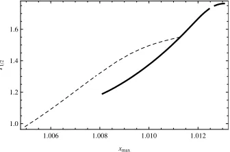
1.006 1.008 1.010 1.012

1.0 1.2 1.4 1.6

xmax T1



2

Fig. 10 Half period of classical halo orbits aboutL2is shown by the dashed line, and the half

1.006 1.008 1.010 1.012 0.000

0.002 0.004 0.006 0.008 0.010 0.012 0.014

xmax zmax

Fig. 11 Classical halo orbits aboutL2shown by dashed line, and artificial halo orbits about

AEPr0 = (1.01134,0,0) with low-thrust accelerationa0= (−0.01,0.0). Heavy dots on both

curves corresponds to stable halo orbits.

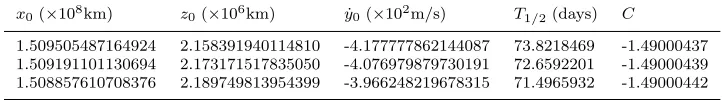
Table 1 Initial condition for stable orbits with a0 = (−0.01,0,0) which corresponds to a

low-thrust acceleration 0.0593 mms−2and low-thrust force 30 mN for a 500 kg spacecraft.

x0(×₁₀8

km) z0(×₁₀6

km) y0˙ (×₁₀2

m/s) T1/2(days) C

1.509505487164924 2.158391940114810 -4.177777862144087 73.8218469 -1.49000437

1.509191101130694 2.173171517835050 -4.076979879730191 72.6592201 -1.49000439

1.508857610708376 2.189749813954399 -3.966248219678315 71.4965932 -1.49000442

According to Floquet theory, the first order or linear stability of periodic orbits is described by the eigenvalues of the monodromy matrixΦ(T). Let the nonlinear system Eq. (1) be written as_X˙ _{=f(X). Since the trace of the Jacobian} ∂f

∂X = 0 [see Eq. (5)], eigenvalues of the monodromy matrix occur in reciprocal pairs [16]. The system is autonomous, so it has +1 as an eigenvalue for a periodic orbit[17]. Thus, two of the eigenvalues of the monodromy matrix are unity, and the stability of the periodic orbit is given by the complex conjugate eigenvalues on the unit circle in complex plane. For artificial unstable periodic orbits, the eigenvalues spectrum of the monodromy matrix is given by

{1,1, λr,1/λr, λi,λ¯i} (17)

For stable periodic orbits, the spectrum of the monodromy matrix is described by

{1,1, λi,λ¯i, λj,¯λj} (18)

7 Conclusions

We have shown the possibility of generating halo orbits, using near-term electric propul-sion system in the circular restricted three body problem around nonequilibrium points by changing these points into equilibrium points with low-thrust acceleration. In par-ticular halo orbits around nonequilibrium points insideL1and beyondL2that require the low-thrust acceleration directed towards sunward are shown to be feasible with such low-thrust propulsion. It is therefore impossible for solar sails, to generate these artifi-cial halo orbits. We have also shown that we may fine tune the initial data provided by the Lindstedt Poincar´e method, for integration of nonlinear equations of motion with constant continuous low-thrust acceleration, to produce closed orbits around artificial equilibrium point using a differential corrector. Stable low-thrust halo orbits for a point beyondL2are also found using a continuation method, while the continuing parameter is chosen as the half period of the halo orbit. These stable halo orbits are realizable with solar electric propulsion and found to be towards L2, while the classical stable halo orbits aroundL2are roughly halfway between the Earth andL2.

8 Acknowledgments

The first author acknowledgments useful discussions with Dr. Thomas J. Waters and Dr. James D. Biggs.

References

1. Farquhar, R. and Kamel, A., “Quasi-periodic orbits about the trans-lunar libration point,”

Celestial Mechanics, Vol. 7, 1973, pp. 458–473.

2. Breakwell, J. and Brown, J., “The ‘halo’ family of 3-dimensional periodic orbits in the

Earth-Moon restricted 3-body problem,”Celestial Mechanics, Vol. 20, 1979, pp. 389–404.

3. Richardson, D. L., “Halo orbit formulation for the ISEE-3 mission,” J. Guidance and

Control, Vol. 3, No. 6, 1980, pp. 543–548.

4. Howell, K., “Three-dimensional, periodic, ‘halo’ orbits,” Celestial Mechanics, Vol. 32,

1984, pp. 53–71.

5. Thurman, R. and Worfolk, P., “The geometry of halo orbits in the circular restricted

three-body problem,” Technical report GCG95, Geometry Center, University of Minnesota,

1996.

6. Richardson, D. L., “Analytical construction of periodic orbits about the collinear points,”

Celestial Mechanics and Dynamical Astronomy, Vol. 22, No. 3, 1980, pp. 241–253. 7. McInnes, C., McDonald, A., Simmons, J., and McDonald, E., “Solar sail parking in

re-stricted three-body systems,”Journal of Guidance, Control and Dynamics, Vol. 17, No. 2,

1994, pp. 399–406.

8. McInnes, A., “Strategies for solar sail mission design in the circular restricted three-body

problem,”Masters Thesis, Purdue University, 2000.

9. Baoyin, H. and McInnes, C., “Solar sail halo orbits at the Sun-Earth artificial L1 point,”

Celestial Mechanics and Dynamical Astronomy, , No. 94, 2006, pp. 155–171.

10. Waters, T. and McInnes, C., “Periodic orbits above the ecliptic in the solar sail restricted

3-body problem,” Journal of Guidance, Control and Dynamics, Vol. 30, No. 3, 2007,

pp. 687–693.

11. Morimoto, M., Yamakawa, H., and Uesugi, K., “Artificial Equlibrium Points in the

Low-Thrust Restricted Three-Body Problem,”Journal of Guidance, Control and Dynamics,

Vol. 30, No. 5, 2007, pp. 1563–1567.

12. Morimoto, M., Yamakawa, H., and Uesugi, K., “Periodic orbits with Low-Thrust

Propul-sion in the Restricted Three-Body Problem,”Journal of Guidance, Control and Dynamics,

13. Betounes, D.,Differential Equations: theory and applications, Springer-Verlag, New York, 2001, pp. 200-205.

14. Battin, R. H.,An Introduction to the Mathematics and Methods of Astrodynamics, AIAA,

Reston, VA, rev. ed., 1999, pp. 573.

15. Kim, M. and Hall, C., “Lyapunov and Halo Orbits aboutL2,”AAS/AIAA Astrodynamics

Specialist Conference, Quebec City, Canada, AAS 01-324, Jul 30-Aug 2, 2001.

16. Broucke, R., Lass, H., and Boggs, D., “A note on the solution of the variational equations

of a class of dynamical systems,”Celestial Mechanics and Dynamical Astronomy, Vol. 14,

No. 3, 1976, pp. 383–392.

17. Whittaker, E.,A treatise on the analytical dynamics of particles and rigid bodies,

Cam-brige University Press, New York, 4th ed., 1999, pp. 398-399.

18. Lara, M., Russel, R., and Villac, B., “Fast estimation of Stable Regions in Real Mode,”

Celestial Mechanics and Dynamical Astronomy, Vol. 42, No. 5, October 2007, pp. 511–515. 19. Villac, B. F., “Using FLI Maps for Preliminary Spacecraft Trajectory Design in

Multi-Body Environments,”Celestial Mechanics and Dynamical Astronomy, Vol. 102, No. 1-3,