Halling, P.J. (2009) Estimation of flattening coefficient for absorption and circular dichroism using simulation. Analytical Biochemistry, 387 (1). pp. 76-81. ISSN 0003-2697
http://strathprints.strath.ac.uk/19249/
This is an author produced version of a paper published in Analytical Biochemistry, 387 (1). pp. 76-81. ISSN 0003-2697. This version has been peer-reviewed but does not include the final publisher proof corrections, published layout or pagination.
Strathprints is designed to allow users to access the research output of the University of Strathclyde. Copyright © and Moral Rights for the papers on this site are retained by the individual authors and/or other copyright owners. You may not engage in further
distribution of the material for any profitmaking activities or any commercial gain. You may freely distribute both the url (http://strathprints.strath.ac.uk) and the content of this paper for research or study, educational, or not-for-profit purposes without prior
permission or charge. You may freely distribute the url (http://strathprints.strath.ac.uk) of the Strathprints website.
Preprint of article published in Analytical Biochemistry387: 76–81.
DOI: 10.1016/j.ab.2009.01.006
Estimation of flattening coefficient for absorption and circular
dichroism using simulation
Peter J Halling
WestCHEM, Dept Pure & Applied Chemistry, University of Strathclyde, Glasgow G1 1XL, UK
[email protected] Tel: +44 141 548 2683 Fax: +44 141 548 4822
ABSTRACT.
The absorbance and circular dichroism (CD) of suspensions is lower than if the same amount of chromophore were uniformly distributed throughout the medium. Several mathematical treatments of this absorption flattening phenomenon have been presented, using various assumptions and approximations. This paper demonstrates an alternative simulation approach, which allows relaxation of assumptions. On current desk-top computers the algorithm runs quickly with enough particles and light paths considered to get answers usually accurate to better than 3%. Results from the simulation agree with the most popular analytical model for 0.01 volume fraction of particles, showing that the extent of flattening depends mainly on the absorbance through a particle diameter. Unlike previous models, the simulation can show that flattening is significantly lower when volume fraction increases to 0.1, but higher if the particles have a size distribution. The simulation can predict the slope of the nearly linear relationship between flattening of CD and the absorbance of the suspension. This provides a method to correct experimental CD data, where volume fraction and particle size are known.
Keywords: protein particles, particle size, software
INTRODUCTION.
Measurements of light absorption or circular dichroism on suspended particles may differ compared with the same amount of chromophore uniformly distributed in solution. A key contribution is the phenomenon of absorption flattening, which has in the past also been termed “shadowing”, “obscuring” and the “sieve effect” [1-14]. (The instrument signal may also be affected by light scattering, which will not be considered further in this paper.) There are several different pictures of the origin of the flattening effect, but all of them relate to the same fundamental cause. Perhaps the easiest is to imagine the appearance of a projection of the suspension in a plane perpendicular to the light path (i.e. as seen by the light entering the suspension). Now, if the particles are sufficiently dilute, there will be parts of this projection that contain no particles at all (i.e. light paths through the suspension that pass entirely
absorb light meeting them. Hence the suspension will have a maximum absorbance, however large the chromophore concentration within the particles or its absorbance coefficient. A slightly different picture considers that because of the random distribution of particles, different light paths through the suspension will pass through particles for different fractions of their length. The average of the absorbance over these various paths will equal that if the some amount of chromophore were uniformly distributed. But the spectrophotometer will average not absorbances but intensities (which are exponential functions of the former). The smaller absorbance (larger intensity) paths will make a disproportionately large contribution to this mean intensity. Hence the final absorbance calculated from the mean intensity will be smaller than the mean absorbance, unless the absorbances through each light path are exactly equal.
If all absorbances are relatively small, it is fairly easy to see that the absorbance reducing effects of the high transmittance light paths (meeting few or no particles) will be weaker. Hence the effect most strongly reduces measured absorbance in regions of the spectrum where the absorbance coefficient is high, flattening the tops of the peaks (the origin of the name). The same phenomenon also affects circular dichroism (CD) spectra, because these show the difference in absorbance for right and left circularly polarised light. Indeed, there has been more interest recently in flattening effects in CD than for simple absorbance. In part this is because in CD light scattering from suspensions has a smaller impact - simple light scattering (of equal magnitude for both polarisations) does not affect the CD signal, provided sufficient light still reaches the detector for it to be measured. Measurements of circular dichroism on suspensions have been widely used in the study of membrane proteins. These must normally be kept in place in membrane fragments in order to retain their native structures. Flattening effects can be significant when measurements are made on the resulting suspensions [5,7,15]. CD measurements are also of interest on other types of small particles in suspension (e.g. [16,17]).
The size of the flattening effect was first analysed in a classic paper by Duysens [1]. Since then there have been a series of approaches to modelling the effect [2-14], which are
discussed in more detail in the Theory section. The literature approaches have used analytical treatments to derive equations that describe the effect, with the use of various simplifying or approximating assumptions. The final equations may be solved analytically or numerically, and their predictions are shown below for comparison. In this paper I will describe and present results from a simulation approach to describe the phenomenon. This would have been computationally extremely expensive or impossible at the time of most of the previous treatments. However, as will be shown, the speed of current computers makes it an attractive option. A simulation approach also makes it relatively easy to relax one or more of the approximations made in relation to the real system.
THEORY
Simulation approach
The basic idea is to simulate the passage of light along the full pathlength through a portion of the sample volume. The appropriate number of particles are placed randomly within the volume, and then an array of possible light paths are examined. For each light path, calculate the fraction of its length that passes through one or more particles, and hence determine the intensity of light that would emerge from that path. From the summed intensities the expected measured absorbance or CD signal of the suspension can be calculated. This may be
compared with the values that would be found if the chromophores were distributed uniformly through the medium (or, equivalently, when every light path had an identical fraction of its length within the particles, equal to their volume fraction).
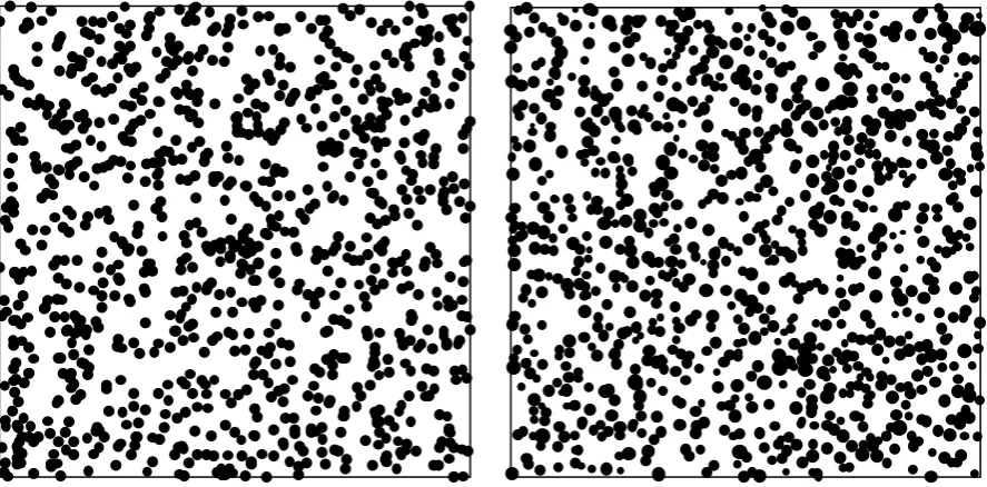
The appearance of the suspension in a projection perpendicular to the light path does not depend on the absolute pathlength, but rather on its ratio to the particle diameter (see examples in Fig. 1). Hence it is convenient to use a dimensionless parameter (L), the
Fig. 1. Simulated appearance of suspension as viewed along light path. Left panel, for φ = 0.01 and L = 20; right panel, for φ = 0.1 and L = 2 with a 20% standard deviation in particle diameters. It is evident that many light rays will not meet any particle at all. The calculated maximum absorbances of the suspension are about 0.13 and 0.15, however large Apart becomes.
analytical treatments, to make this dimensionless by multiplying by the particle diameter. The result, which is equal to the absorbance measured through a diameter of the particle, is
denoted by Apart. To simulate the effect on CD measurements, we use the corresponding CD signal for a light ray that passes through the diameter of one particle, CDpart. This is by definition equal to Apart,L – Apart,R, the difference in absorbances for left and right circularly polarised light. To find the individual terms, we make use of the fact that the average intensity transmitted by the particle (as appearing in the definition of Apart) is equal to the mean of transmitted intensities of the two polarisations. This allows us to derive:
⎟
⎟
⎠
⎞
⎜
⎜
⎝
⎛ +
+
=
⎟
⎟
⎠
⎞
⎜
⎜
⎝
⎛ +
+
=
−
2
10
1
log
2
10
1
log
,,
. CDpart
part R
part part
CD part
L
part
A
A
A
A
Because all four inputs to the simulation are dimensionless, all lengths considered in the simulation will also be dimensionless multiples of the particle diameter.
1. Set up a simulated volume, with pathlength L, which will be taken as the z-axis direction. The total volume (V) is chosen to contain the number of particles to be included in the simulation (N, e.g. 1000), by V = N.π/(6.φ). Note that the value of N does not affect the nature of the system being simulated (which depends only on φ and L), but just the size of the portion that is included in the simulation. N must be large enough that this portion is representative of the system as a whole. Note also that V will also be dimensionless, based on division by the cube of the particle diameter. To achieve the required volume, equal widths of the simulation region are then set in the x and y directions (=√(V/L).
2. Place the required number of spherical particle centres randomly throughout the simulated volume, not allowing a new particle to overlap a previous one, or to overlap the ends of the volume in the z direction (assumed to be sample container walls). Overlap of the simulation volume edges in the x and y directions are allowed, as these are merely arbitrarily chosen limits to the simulation volume.
3. Consider an array of light ray paths along the z direction, uniformly distributed in the x-y plane (e.g. 32 X 32 raster, giving a total of 1024). For each light ray, calculate the total length of its path through particles. The algorithm does this by simply
considering each simulated particle in turn, seeing if it intersects that ray. For a light ray that has coordinates xr and yr such that it passes through a particle of radius R, at a distance r from the particle centre (= √[(xr-xp)2+(yr-yp)2]), the light path length through the particle is 2√(R2-r2). (This neglects refraction at the particle-medium surface.) All such contributions to the given light ray are summed. Light paths are placed at least one particle radius from the x and y edges, so they could not meet any particles centred outside the simulated volume.
5. Calculate the average transmitted intensity from all these light paths, for each possible combination of Apart and CDpart values, and hence the (flattened) absorbances of the suspension (Asus). Calculate the CD signal of the suspension (CDsus) as the difference in Asus values for left and right polarised light.
6. Calculate the reference absorbance (Asol) or CD signal (CDsol) if the absorbing material were uniformly distributed (no flattening). First calculate the average across all light paths of the path length through particles. This should be very close to the product φ.L, and is found to be so, although the random element in the simulation means they differ slightly. Then multiply by the various possible Apart or CDpart values. 7. For the estimation of the flattening coefficient (QA) as Asus/Asol, the Asol values might
be calculated as Apart multiplied either by φ.L, or by the average path length through particles (as under step 6). The QA values from replicate simulations were found to be rather closer to each other using the latter approach. The same applied to QCD values, calculated as CDsus/CDsol. Hence the latter approach has been used to give the results shown here. The random element in the simulation results in a set of light ray paths that have a slightly larger or smaller average length in particles. Essentially this means they are characteristic of a slightly different value of φ, compared with that input.
A number of assumptions and approximations are made in this treatment, but it should be possible to relax these, at the expense of a more complicated calculation.
• The current simulation treats light passage through the suspension in terms of classical geometric optics. As such it will not be valid in cases where the particles sizes are not significantly larger than the wavelengths of the light used [4, 8].
• Light paths are treated as straight lines all though the suspension, neglecting possible refraction at the particle surfaces.
• It is assumed the chromophore is equally distributed between the particles, and evenly distributed within each.
the last of these is demonstrated below. Other extensions are under development. To get reliable results for the more complicated cases it may be necessary to include more particles and/or light paths in the simulation, with a corresponding increase in calculation time.
Re-arrangement and re-parameterisation of literature equations for comparison
In order to compare the results of the simulation approach with those from literature
equations, it is necessary to convert these to use the same dimensionless input variables (i.e. Apart, φ and L). One useful relationship here is that Asol = Apart.φ.L, since other treatments show the relationship of Asol to their input values.
A series of papers derive essentially the same equation by different routes and arguments [1-4, 10]. Using the symbols of Naqvi et al [10], the procedure is to calculate first the parameter α, by
10
ln
.
.
.
n
d
ε
α
=
(1)where ε is the extinction (absorbance) coefficient of the chromophore, n is its concentration within the particle and d is the particle diameter. It is clear that α equals Apart as defined above multiplied by ln10. The factor of ln10 appears because the treatment essentially specified absorbance as ln(Io/I), which is indeed used as its definition in the earlier papers, rather than log(Io/I) as standard nowadays. From α, calculate β, the “average transmission of a particle”, as
(
)
[
]
2
1 1 2
α α
β = − + e−α (2)
Finally, calculate QA (AD/AC in their symbols) by
(
)
α β 2 1
3 −
= =
C D A
A A
Q (3)
Hence the model predicts that QA depends only on Apart, and is independent of φ and L. Some of the derivations explicitly assume that φ << 1.
l c N N n N n n sus p p p ch p
e
A
. . .0 2 ) (
10
.
2
1
2 2 ε σ μπ
σ
− = − −∑
=
(4)with ch p ch ch p ch p N N N N N N N ≈ ⎟⎟ ⎠ ⎞ ⎜⎜ ⎝ ⎛ − = = 1 1 . and σ μ
However, examination of their derivation shows that the expression actually gives Isus/Io, so Asus should be calculated as the negative log of this value. In this equation:
Np is the total number of particles in the sample cell
Nch is the number of light “channels” through the sample – these are to be chosen so they have “a cross-section corresponding to the size of the absorbing particles”.
εp is the “molar absorptivity of the particles” cp is the “molar concentration of the particles” l is the sample pathlength
One stated limit on validity is that Np/Nch > 2.
To relate this equation to the input values used in the simulation, we introduce (and later cancel) the area A of the suspension in the x-y plane, facing the light beam. Now we can interpret the rule stated above for choosing channel size as meaning Nch = A/d2, where d is the particle diameter. (An alternative interpretation would be Nch = 4A/πd2, giving slightly
different relationships.) We can also write Np = np.A.l, where np is the number of particles per unit volume in the suspension. But np can also be related to φ by φ = np.πd3/6. Hence we obtain Np/Nch = (6/π).φ.L. Wittung et al [9] also present the relationship Asol = εp.cp.l, so we can replace the entire group (Nch/Np).εp.cp.l by π.Apart/6. Hence we calculate QA by
⎥
⎥
⎦
⎤
⎢
⎢
⎣
⎡
−
=
=
− = − −∑
6 . . 0 2 ) (10
.
2
1
log
.
.
.
1
2 2 partp n A
N n n part sol sus A
e
L
A
A
A
Q
π σ μπ
σ
with π φ π φ π φ σ π φ μ ch p ch N L N L N L
L 6. . .
and . . 6 1 1 . . . 6 and . .
6 ≈ =
⎟⎟ ⎠ ⎞ ⎜⎜ ⎝ ⎛ − = =
Thus QA is predicted to depend on Apart, φ.L, and Nch. The stated limit on validity becomes
φ.L > 1. For the Apart and φ.L ranges studied, the influence of Nch was found to be small when it is greater than 20.
Bustamante and Maestre [8] derive the following equations (their 12, and the following expression for q, using their 11 to expand Vf):
(
)
⎥⎦
⎤
⎢⎣
⎡
−
−
=
=
2.
.
2
1
.
303
.
2
1
λ
k
q
a
A
A
Q
sol susA , with
T w a
V
M
l
k
N
W
q
.
.
.
.
.
λ
2=
(6)where
a is the absorption cross section of the chromophore, with dimensions of length squared q is “the probability of finding a particle in the volume defined by a light pencil”
k is a “proportionality constant whose exact value is of no consequence”, which they take as 1
λ is the wavelength of the light used
W is the total weight of the absorbing material in the solution Na is Avogadro’s number
l is the pathlength
Mw is the molecular weight of the absorbing particles VT is the total volume of the solution
⎟ ⎠ ⎞ ⎜ ⎝ ⎛ − ⎟⎟ ⎠ ⎞ ⎜⎜ ⎝ ⎛ − = 1 . . . 1 . 2 . . . 303 . 2 1 2 c l k L A
QA part
λ
φ
(7)
Thus QA is predicted to depend on the two dimensionless groups Apart.φ.L and k.λ2.l.c, where one limit to validity is that the latter must be less than 1.
There are fewer equations in the literature for flattening of CD spectra of spherical particles. Gordon & Holzwarth [2] present
⎥
⎦
⎤
⎢
⎣
⎡
⎟⎟
⎠
⎞
⎜⎜
⎝
⎛
−
−
=
=
m
q
A
T
A
m
q
Q
Q
sol p sol B CD.
.
2
.
3
exp
.
.
2
(8)where q is the volume fraction of particles (i.e. φ), m = (3 X pathlength)/(4 X particle radius) (i.e. 3L/2), and Tp is an alternative symbol for β calculated as in equation 2 above.
Substitution leads to
( )
[
β
α
α
−
−
=
3
exp
CD
Q
]
(9)Urry [3] presents an algorithm for the calculation of QCD, by successive use of equations 44 and 45, 46, 47 and 42 (as numbered in that paper). For comparison with the present treatment, the scattering terms in equation 42 are set to zero. The input values to the algorithm are Apart, CDsol and Asol (using my symbols). However, a test using a range of realistic values indicates that the latter two have almost no effect on the calculated QCD. Furthermore, the QCD values obtained are found to agree within 0.1% with those calculated using equation 9 above. Hence they are not treated separately below.
Bustamante and Maestre [8] derive the relationship:
QCD = 2(QA– 0.5) (10)
RESULTS AND DISCUSSION
The simulation has been implemented as a Visual Basic macro attached to an Excel spreadsheet. The latest version of this will be supplied without restriction on request to the author. Running a simulation with 1000 particles and 1024 light paths takes about 3 s on a standard PC. Replicate simulations with these values usually agree with standard deviations in QA and QCD values of <3%, often much smaller. Larger deviations are observed in some cases, especially where the values of Asus are very large, or QCD is very small. Standard deviations are shown as error bars on the graphs presented (often smaller than the points). Increasing the number of particles to 5000 seemed to have little effect on the standard deviations obtained, whereas an increase to 4098 (64 X 64) light paths typically reduced the standard deviation to about half.
Simulations have been run for input values in the following ranges: Apart. 0.001 to 5; φ 0.01 to 0.1; L 2 to 2000; CDpart 0.00001 to 0.1 (and no more than 10% of Apart). The effects of φ; L and CDpart on QA and QCD are found to be relatively small, with Apart having the major
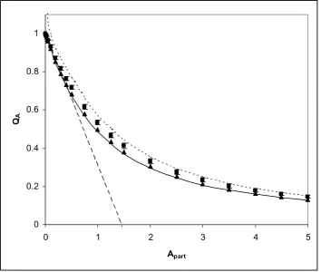
influence. Fig. 2 shows the dependency of QA, with simulation results indicated by points. For comparison, lines show the predictions of the 3 literature models above. As can be seen, the simulation points for φ = 0.01 agree well with equation 3, as might be expected in the low φ
limit. For φ = 0.1 the values of QA obtained by simulation are slightly but significantly larger (i.e. less flattening). One contributing effect here is the greater restriction on particle locations by others present in the suspension (i.e. an excluded volume effect). This makes the
distribution of particles across light paths rather more uniform as φ increases. It may be helpful to think of behaviour at very high φ, approaching the close packed limit, when the particle centres must be arranged ever closer to a regular lattice.
The model of equations 4 and 5 is only applicable for the φ = 0.1 case here, because of the requirement that φ.L > 1. The line shows reasonable agreement with the points at high Apart, but is significantly higher at lower values. It is likely that one of the approximations used in the derivation breaks down, particularly as the equations give physically impossible values of QA > 1 at the lowest Apart values. The model of equations 6-7 gives an almost linear
the range of input values studied here. One relevant factor may be that the derivations of both these alternative models seem to assume that the numbers of particles encountered by a light ray can be approximated by the normal distribution. This will only be correct where the mean numbers are large – in many cases low numbers and a Poisson distribution will hold.
0 0.2 0.4 0.6 0.8 1
0 1 2 3 4
Apart
QA
[image:14.595.74.429.169.469.2]5
Fig. 2. Predicted QA vales from simulation and literature equations.
Simulations for L = 20, with φ of 0.01 (triangles) and 0.1 (squares). Most error bars are smaller than the size of the points, but they are just visible for the square points at medium Apart values. Lines show results from equations 1-3 (solid); 4 and 5, with φ.L = 2 and Nch = 100 (dotted); 6 and 7, with φ.L = 0.2 and k.λ2.l.c = 0.25 (dashed). The latter value was adjusted so that the line agrees with the simulation points and equations 1-3 at the low Apart limit.
No significant effects on the simulation results were found on increasing L, until φ.L values were greater than 2. After that, QA values seemed to become larger for the higher Apart values, although the standard deviations also increased substantially. In this range Asol and Asus
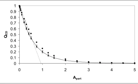
Turning to QCD, the simulation results indicate that the major influence is again Apart, as shown in Fig 3. Just as with QA, there is a small but significant increase in QCD on raising φ from 0.01 to 0.1. No significant effect of CDpart on QCD was detected anywhere in the region studied. Similarly there was no effect of L until φ.L became greater than 2. At larger values there was an indication of higher QCD for larger Apart values, although with the same increased standard deviations and excessive Asus values as for QA. The literature model of equations 1, 2 and 9 agrees well with the simulation results for φ = 0.01, indicating again that it holds for the low φ limit. The model of equations 6, 7 and 10 can be adjusted to fit in the initial region of more or less linear decline in QCD, but cannot describe the curvature at higher Apart values.
0
0.1
0.2
0.3
0.4
0.5
0.6
0.7
0.8
0.9
1
0
1
2
3
4
5
A
part [image:15.595.75.546.277.563.2]Q
CDFig. 3. Predicted QCD values from simulation and literature equations.
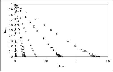
In our previous treatment of CD measurements on suspensions of immobilised enzyme particles [11], we used a semi-empirical model based on the assumption that QCD was linearly related to the measured absorbance of the suspension. (In this paper we defined the “flattening coefficient” in the same way as Wallace and Mao [5], that is equal to (1-QCD) as used in the current paper and much of the rest of the literature.) Fig. 4 shows that this approximation is quite good for a range of input values, with QCD falling linearly from 1 for Asus = 0. The slope of the line (the adjustable parameter in our previous treatment) is strongly dependent on the values of φ and L. There may be some deviation from linearity as QCD approaches zero, which also corresponds to a predicted maximum possible value of Asus (because absorption
flattening prevents this value being exceeded).
0 0.1 0.2 0.3 0.4 0.5 0.6 0.7 0.8 0.9 1
0 0.5 1 1.5
Asus
[image:16.595.73.471.294.548.2]QCD
Fig. 4. Relationship between QCD and Asus from simulations.
Points are for the series of Apart values up to 5, and the corresponding CDpart values, as for Fig. 3. The series are for: φ = 0.01, L = 2 (filled squares); φ = 0.01, L = 20 (open squares); φ = 0.1, L = 2 (filled circles); φ = 0.05, L = 10 (open circles); φ = 0.1, L = 10 (filled triangles); φ = 0.01, L = 200 (open triangles). Both x and y error bars are shown, where larger than the size of the points.
given diameters with deviations about the mean, taken randomly from a normal distribution with an appropriate variance. Table 1 compares the QA and QCD values found for uniform particle sizes and for a standard deviation of 20% of the mean. As can be seen both QA and QCD are significantly smaller when the particles are not equal in size.
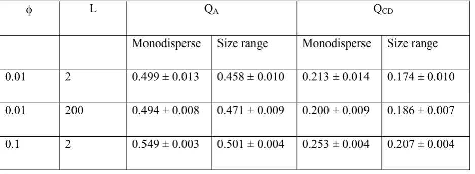
Table 1. Effect of particle size distribution on QA and QCD.
φ L QA QCD
Monodisperse Size range Monodisperse Size range 0.01 2 0.499 ± 0.013 0.458 ± 0.010 0.213 ± 0.014 0.174 ± 0.010 0.01 200 0.494 ± 0.008 0.471 ± 0.009 0.200 ± 0.009 0.186 ± 0.007 0.1 2 0.549 ± 0.003 0.501 ± 0.004 0.253 ± 0.004 0.207 ± 0.004
Values of QA and QCD for Apart = 1, for case with either: a) all particles of identical size, or b) with diameters having a normal distribution with the same mean and a standard deviation of 20% of the mean. Results are shown as mean ± standard deviation from 5 replicate runs. All simulations were performed using 64 X 64 light paths, for greater accuracy. All differences between monodisperse particles and those with a size range are statistically significant at levels ranging from 1.2% down to 10-6%.
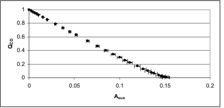
The relationship between QCD and Asus suggests an approach to use the simulation to handle experimental data. It will usually be possible to estimate φ and L from other measurements on the particle suspension. That should allow construction of a plot of QCD vs. Asus like that of Fig. 4. Then the measured Asus of the suspension (e.g. obtained from the HT signal on a CD spectropolarimeter) can be used to estimate QCD from the plot. Finally this can be used to correct the measured CD signal. In this approach the parameter Apart, as used in the
To illustrate how the simulation method can be used with experimental data, I have taken a data set from our previously published measurements [11]. The conditions of measurement were used as inputs to a simulation giving the plot of Fig. 5. The HT data from the
spectropolarimeter was used to estimate Asus values, which were then used to obtain
corresponding QCD values, using a smooth interpolation line on Fig. 5. These QCD values are in turn used to correct the CD spectrum, as shown on Fig. 6. The resulting spectrum should be a sounder basis for evaluating the secondary structure in the protein, and other analysis.
0 0.2 0.4 0.6 0.8 1
0 0.05 0.1 0.15 0.2
Asus
[image:18.595.74.461.263.450.2]QCD
Fig. 5. Relationship between QCD and Asus used to correct experimental data.
-10000 -5000 0 5000 10000
190 210 230 250
Wavelength/nm
C
D
/de
gc
m
2 dm
ol
[image:19.595.75.380.72.249.2]-1
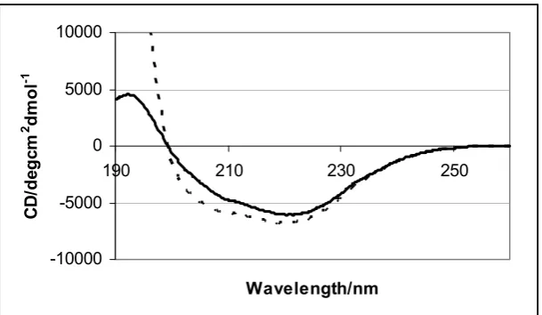
Fig. 6. Correction of circular dichroism spectrum using simulation results.
Measurements were for a suspension of silica-subtilisin in aqueous buffer, and had been converted to the usual CD units using the measured protein concentration in the cell (solid line) [11]. The output for the applied high tension (HT) voltage from the spectropolarimeter was used to estimate the spectrum of Asus values for this sample (with some allowance for scattering using the HT data for a suspension of the same silica particles without enzyme immobilised on them). These Asus values were then used to obtain corresponding QCD values, using Fig. 5. Finally the table of QCD values was used to produce the corrected CD spectrum (dotted line), calculated as the measured CD divided by QCD. The “corrected” line is not shown at the shortest wavelengths, as here the estimated values of QCD become very small, so that small absolute errors in them will have major effects on the size of the correction, and the results are probably not reliable.
CONCLUSION
A simulation approach is an effective method to estimate the extent of flattening when making absorption or CD measurements on particle suspensions.
REFERENCES
[2]D.J. Gordon, and G. Holzwarth, Artifacts In The Measured Optical Activity Of Membrane Suspensions. Archives Of Biochemistry And Biophysics 143 (1971) 481-488.
[3]D.W. Urry, Protein Conformation In Biomembranes: Optical Rotation And Absorption Of Membrane Suspensions. Biochimica et Biophysica Acta 265 (1972) 115-168.
[4]P. Latimer, The deconvolution of absorption spectra of green plant materials - improved corrections for the sieve effect. Photochemistry and Photobiology 38 (1983) 731-734. [5]B.A. Wallace, and D. Mao, Circular-dichroism analyses of membrane-proteins - an
examination of differential light-scattering and absorption flattening effects in large membrane-vesicles and membrane sheets. Analytical Biochemistry 142 (1984) 317-328.
[6]C.L. Teeters, J. Eccles, and B.A. Wallace, A Theoretical-Analysis Of The Effects Of Sonication On Differential Absorption Flattening In Suspensions Of Membrane Sheets. Biophysical Journal 51 (1987) 527-532.
[7]B.A. Wallace, and C.L. Teeters, Differential Absorption Flattening Optical Effects Are Significant In The Circular-Dichroism Spectra Of Large Membrane-Fragments. Biochemistry 26 (1987) 65-70.
[8]C. Bustamante, and M.F. Maestre, Statistical effects in the absorption and optical activity of particulate suspensions. Proc. Natl. Acad. Sci. USA 85 (1988) 8482-8486.
[9]P. Wittung, J. Kajanus, M. Kubista, and B.G. Malmstrom, Absorption Flattening In The Optical-Spectra Of Liposome-Entrapped Substances. FEBS Letters 352 (1994) 37-40. [10]K.R. Naqvi, T.B. Melo, B.B. Raju, T. Javorfi, and G. Garab, Comparison of the
absorption spectra of trimers and aggregates of chlorophyll a/b light-harvesting complex LHC II. Spectrochimica Acta Part a-Molecular and Biomolecular Spectroscopy 53 (1997) 1925-1936.
[12]E. Castiglioni, S. Abbate, G. Longhi, and R. Gangemi, Wavelength shifts in solid-state circular dichroism spectra: A possible explanation. Chirality 19 (2007) 491-496. [13]E. Castiglioni, S. Abbate, G. Longhi, R. Gangemi, R. Lauceri, and R. Purrello,
Absorption flattening as one cause of distortion of circular dichroism spectra of Delta-RuPhen(3).H2TPPS complex. Chirality 19 (2007) 642-646.
[14]E. Castiglioni, F. Lebon, G. Longhi, R. Gangemi, and S. Abbate, An operative approach to correct CD spectra distortions due to absorption flattening. Chirality 20 (2008) 1047-52.
[15]S.M. Kelly, T.J. Jess, and N.C. Price, How to study proteins by circular dichroism. Biochimica et Biophysica Acta 1751 (2005) 119 - 139.
[17]B. Sarmento, D.C. Ferreira, L. Jorgensen, and M. van de Weert, Probing insulin's secondary structure after entrapment into alginate/chitosan nanoparticles. European Journal of Pharmaceutics and Biopharmaceutics 65 (2007) 10-17.
[16]C.S. Braun, G.S. Jas, S. Choosakoonkriang, G.S. Koe, J.G. Smith, and C.R. Middaugh, The structure of DNA within cationic lipid/DNA complexes. Biophysical Journal 84 (2003) 1114-1123.
[18]B. Castillo, V. Bansal, A. Ganesan, P. Halling, F. Secundo, A. Ferrer, K. Griebenow, and G. Barletta, On the activity loss of hydrolases in organic solvents: II. A mechanistic study of subtilisin Carlsberg. BMC Biotechnology 6:51 (2006).
[19]A. Ganesan, A.A. Watkinson, and B.D. Moore, Circular dichroism measurements of the structure and stability of anthrax protective antigen adsorbed onto aluminium
adjuvant. American Association of Pharmaceutical Scientists Journal 9 (2007) abstract 667. http://www.aapsj.org/abstracts/NBC_2007/NBC07-000667.PDF.