A three-dimensional finite element model of maximal grip loading in the human wrist

(1)

A 3D finite element model of maximal grip loading in the human wrist

Magnús K. Gíslason1*, David H. Nash1, Alexander Nicol1, Asimakis Kanellopoulos1, Marc Bransby-Zachary2, Tim Hems3, Barrie Condon2, Benedict Stansfield4,

1

Bioengineering Unit, Wolfson Building, University of Strathclyde, 106 Rottenrow,

Glasgow,

G4 0NW, UK

2_{Southern General Hospital, Glasgow, UK}

3

Victoria Royal Infirmary, Glasgow, UK

4

Glasgow Caledonian University, Glasgow, UK

*_{Corresponding author. Bioengineering Unit, Wolfson Building, University of}

Strathclyde, 106 Rottenrow, Glasgow, G4 0NW, UK. Tel.: +44 (0)141 548 3228; fax:

+44 (0)141 552 6098

(2)

Abstract Aims

To create an anatomically accurate three-dimensional finite element model of the wrist, applying subject specific loading and quantifying the internal load transfer through the joint during maximal grip.

Methods

For three subjects, representing the anatomical variation at the wrist, loading on each digit was measured during a maximal grip strength test with simultaneous motion capture. Internal metacarpophalangeal joint load was calculated using a biomechanical model. High resolution MR scans were acquired to quantify bone geometry. Finite element analysis was performed, with ligaments and tendons added, to calculate internal load distribution.

Results

For maximal grip the thumb carried the highest load, average of 72.2±20.1 N in the neutral position. Results from the finite element model suggested that the highest regions of stress were located at the radial aspect of the carpus. Most of the load was transmitted through the radius, 87.5% opposed to 12.5% through the ulna with the wrist in a neutral position.

Conclusions

A fully three-dimensional finite element analysis of the wrist using subject specific

anatomy and loading conditions was performed. The study emphasises the importance of modelling a large ensemble of subjects in order to capture the spectrum of the load transfer through the wrist due to anatomical variation.

(3)

A 3D finite element model of maximal grip loading in the human wrist

Magnús K. Gíslason1*, David H. Nash1, Alexander Nicol1, Asimakis Kanellopoulos1, Marc Bransby-Zachary2, Tim Hems3, Barrie Condon2, Benedict Stansfield4,

1

Bioengineering Unit, Wolfson Building, University of Strathclyde, 106 Rottenrow,

Glasgow, G4 0NW, UK

2_{Southern General Hospital, Glasgow, UK}

3_{Victoria Royal Infirmary, Glasgow, UK} 4

Glasgow Caledonian University, Glasgow, UK

1. Introduction

The wrist is an anatomically complex joint. It is composed of 8 carpal bones assembled

in a two row structure. In the proximal row are the (from radial to ulnar) scaphoid,

lunate, triquetrum and pisiform. The pisiform is a sesamoid bone and plays no part in the

overall load transfer. The distal row comprises of the (from radial to ulnar) trapezium,

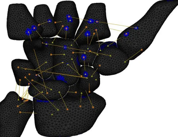
trapezoid, capitate and hamate [1]. Bone and ligamentous geometry are illustrated in

Figure 1. There has been considerable debate about how load is transmitted through the

joint over the last few decades. In 1981 some of the first wrist cadaveric measurements

were carried out by Palmer and Werner [2] who used a load cell in order to establish the

load transfer ratio between the radius and ulna. Other cadaveric studies followed in order

(4)

and Tencer et al [3-5] respectively performed cadaveric experiments using pressure

sensitive films, placed at the articulating surface of the carpal bones in order to measure

the contact pressures. The results from these cadaveric studies have shed light on how the

wrist responds under loading, but concerns can be raised about the measuring procedures.

Cadaveric measurements are difficult to perform. The wrist is a very delicate joint and by

performing an invasive measurement it is possible that the researcher could be perturbing

the joint as the dissection is carried out. Another issue with cadaveric studies is that after

the specimen has been dissected and set up for experimental work, it is not possible to

redo the experiment with modified parameters. This, along with difficulty in obtaining

cadaveric specimens, makes these experiments time consuming and expensive to

perform. Several theoretical models [6,7] of the wrist exist. These have been developed

mostly by creating a Rigid Body Spring Model (RBSM) to calculate the force

transmission and displacement between multiple non deformable bodies using a series of

springs with known stiffness. The geometry of the wrist makes such theoretical models

difficult to create. Finite element models of the wrist have been created, but most have

focussed on a particular sub region of the joint, in particular the interaction between the

radius, scaphoid and the lunate, not representing the whole joint. Exceptions to this

include the work of Carrigan et al. in 2003 [8] who developed a three-dimensional FE

analysis of the carpus (without metacarpals). In this work the bones were modelled as

‘hollow’ cortical shells with only a small number of the ligaments included. To obtain

convergence of this model it was necessary to constrain each carpal bone with a system

of non-physiological constraints. None of the models proposed in the literature used

(5)

The aim of the current study was to develop a fully-representative three-dimensional

finite element model of the entire wrist joint in order to study the transmission of force

through the normal carpus during a maximal grip activity. A major consideration was the

use of experimental biomechanical data which were obtained to provide ‘real’ boundary

conditions for the model.

2. Methods

2.1 Subjects

The wrists of three subjects were studied. The three subjects (2 females and 1 male who

all were young and healthy with average age of 26.3, ranging from 24-28 years) were

selected from a group of 10 subjects who had MRI scans of the wrist. The subjects were

selected to represent a range of wrist geometrical configurations, representing a range of

wrist types proposed by Craigen and Stanley in 1995 [9] who suggested that the

kinematics of the carpal bones varied depending on the rotational behaviour of the

scaphoid.

2.2 Activity

The subjects performed a maximal strength grip with one finger on each force transducer

(Figure 2). This was performed in the neutral, radially deviated and ulnarly deviated

(6)

2.3 Anatomical data collection

The subjects were taken for an MRI scan at the Southern General Hospital in Glasgow.

The subjects were scanned with their hands in three positions; neutral, radial deviation

and ulnar deviation. The in-plane resolution of the MRI scan was 230x230µm and the

slice thickness was 700µm. The image size was 512x512 pixels. The imaging consisted

of 92 axially sliced scans ranging from the distal end of the radius and ulna to the

proximal third of the metacarpals, a length in total of 63.7mm. The wrist of each subject

was splinted while the imaging took place in order to keep the wrist as still as possible to

minimise noise and maximise image quality.

2.4 Biomechanical data collection

Realistic external loading conditions must be applied to make the results of FE models

valid. External loads were measured using individual finger transducers (Nano 25-E and

Nano 17, ATI Industrial Automation Inc, USA) (Figure 2). The locations of the joint

centres for each digit were determined from the position of skin mounted markers and

from anatomical features, identified from static calibration trials. From the force

transducer outputs, the inter-segmental loadings in terms of forces across the joints were

calculated. Load was then distributed to the internal structures (tendons, ligaments and

bones) at each joint using an inverse dynamic approach that used an optimisation criteria

that minimised the maximum stress in any of the soft tissue structures as described by

Fowler and Nicol [10,11]. The biomechanical model included all the tendons crossing

(7)

excluded, flexor carpi radialis, flexor carpi ulnaris, extensor carpi radialis longus,

extensor carpi radialis brevis and extensor carpi ulnaris, as the attachment points of these

tendons were at the proximal end of the metacarpals. These tendons were included in the

FE model. This process used real external loading data and person specific anatomical

data thus providing physiologically relevant loading information.

2.5 Finite element model

2.5.1 Mesh generation

The MRI scans were imported into Mimics software (Materialize, Belgium) where edge

detection of the bones was carried out. By using the ‘masking technique’ all the bones

and articulating cartilage were manually identified from each slice, thus creating a layer

of contour surfaces in a plane perpendicular to the axis of the scan. Three-dimensional

surface objects were created of each bone by combining the contours. Meshing was

carried out using triangular elements on the surface objects using an automatic procedure.

To remove surface roughness caused by the digitisation process, a smoothing function

was applied which took each node point and changed its position in relation to the

positions of the adjacent node points. The consequence of this procedure was a volume

reduction within the bones. By recalculating the bone mask, based on the smoothed 3D

object, it was possible to return to the original scans and compensate for the volume

reduction. This became an iterative process, which was carried out until the volume

change from ‘before’ to ‘after’ applying the smoothing function became negligible. The

(8)

ranged from 1.91 elements/mm2 – 3.93 elements/mm2 (average of 2.73 elements/mm2). Various indicators were used to identify badly shaped triangles such as the area ratio, the

skewness defined as the ratio between the triangle and an equilateral triangle with the

same ascribed circle and the equi-angle skewness which was defined as

⎟ ⎠ ⎞ ⎜ ⎝ ⎛ − − 60 180 180 ; 60

min α β (1)

where was the smallest angle of the triangle and was the largest angle of the triangle.

Ideally all the ratios would have been 1, where that would have described an equilateral

triangle. In practice it is difficult to create a mesh using only equilateral triangles. The

minimum value used for the meshing was 0.4. This value was considered to be acceptable

based on the characterisation of equi-angle skew factor of Rábai and Vad in 2005 [12].

The mesh was refined by manually deleting and creating triangles. A histogram was

plotted of the mesh quality indicators and visually evaluated before accepting the surface

mesh quality. The meshes were then exported from Mimics and imported into Abaqus (v.

6.6-1, Simulia, USA) where volume elements were created from the surface elements.

The volume elements were 10 node solid tetrahedral elements (C3D10). For this method

of implementation the volume element shape is determined by the surface element shape

which could possibly lead to the creation of distorted elements [13]. With modern mesh

generators, the robustness of the algorithm minimizes the risk of that happening.

However, the following checks were carried out on the mesh to make sure the elements

were of sufficient quality: Shape factor, minimum face angle, maximum face angle,

aspect ratio. If an element showed signs of distortion, the surface mesh was altered and

(9)

2.5.2 Bone material property assignment

It was not possible to derive the stiffness of each element of bone based on the greyscale

value from the MR images. Areas of different stiffness were visually identified from the

scans, within Mimics. This was performed by eroding the mask containing the bone and

the articulating cartilage, thus creating areas of different stiffness using Boolean

operators. These areas represented the hard cortical shell, the soft cancellous bone, two

transition regions bridging the stiffness values between the hard cortical shell and the soft

cancellous region, and finally, the cartilage. The stiffness values can be seen in Table 1.

The values for cortical bone were taken from Rho et al. [14] and for cancellous bone

from Kabel et al. [15]. The values for the two transition stiffness regions were estimated

and followed a modulus-density power curve proposed by various empirical studies [e.g.

16].

2.5.3 Model assembly

The volumetric elements with the bone material property definitions were imported into

Abaqus where the assembly took place. The ligaments and tendons were modelled as non

linear spring elements. Material properties of the soft tissues were taken from the

literature. Material testing data were found for 26 ligaments [17-29]. All major ligaments

were included in the model. The attachment points were estimated from various

(10)

ligament origins and insertions in a live subject. The origins and insertion points of

ligaments are diverse in nature, with multiple fibre attachment points. To make the

modelling of ligaments possible they were applied as single elements, but with a

distributed origin and insertion achieved by linking adjacent node points.

For ligaments that did not have published material parameters, it was assumed that the

properties of the neighbouring ligaments would apply. An exception to this was for the

transverse metacarpal ligaments which were modelled as being stiff to prevent large

relative movements between the metacarpals.

The non linear curves of the ligaments were generated using the following points:

• Zero stress = zero strain

• Non-linear ‘toe’ region up to 15% of max strain, called .

• Linear curve from 15% max strain to max strain with same slope at the boundary

between the linear and nonlinear regions, based on the formula below derived

from results of Logan and Nowak [25].

(2)

Where a_,b_{are constants,}F _{the force and}x _{the strain.}

All tendons in the fingers that run across the wrist were modelled in the biomechanical

model for calculating the MCP joint loading. In addition the intrinsic tendons were

modelled in the FE simulation. The contributions from the wrist flexors (flexor carpi

radialis and flexor carpi ulnaris) and extensors (extensor carpi radialis longus and brevis

(11)

constraints, with moment arms taken from Horii et al. [31] for the joint position defined

by the MRI scan. Thus all tendon loading was included in the load distribution

calculations. The material properties of the tendons were taken from a material study of

the wrist tendons carried out at the University of Strathclyde [32]. The ligaments and

tendons were modelled as non linear to improve physiological relevance.

There were clear limitations in the ability of the ligament and tendon structures modelled

to offer load resistance perpendicular to their lines of action. This is a simplification of

the action of these structures. The lines of action of the structures were examined during

the simulations and only minor intrusions of them into the bone were observed. It was

therefore concluded that using this representation of the ligaments and tendons was

justifiable as it provided a physiological representation of the main resistance

(longitudinal loading) and minimal compromise of the model integrity.

The number of elements in each assembly of bones in the wrist model ranged from

172,413 to 274,261 (average 228,771) with element density ranging from 6.58 to 9.07

elements/mm3 (average of 7.74) per bone for all the models.

The models were solved using Abaqus explicit solver v6.6-1 and run on a 4 dual 2 GHz

processor cluster with 4Gb of RAM. The analysis took 25-30 hours of CPU time for each

of the models. The 3 models were run using the explicit solver with a total simulated

(12)

2.5.4 Boundary conditions

The action of the external applied loads and the digital extrinsic muscles on the wrist

joint were accounted for by the joint contact loads defined at the metacarpals. These

three-dimensional metacarpal forces were applied over the distal surface of each

metacarpal as a set of boundary conditions.

The proximal surface of the radius and ulnar were constrained by allowing no

displacement or rotation in any direction. The proximal ends of the radius and ulnar were

assumed to be completely rigid.

2.5.5 Contact modelling

The contact modelling using the explicit solver, assumed that all the exterior elements

were in contact. There was therefore no need for a predefined notion of where the contact

surfaces lay. The bones were translated until they were touching their adjacent bone

surface.

A surface-to-surface contact was established between the bones using the ‘hard contact’

algorithm based on

(13)

where p was the contact pressure and h was the overclosure between the surfaces. The

contact modelling was implemented in Abaqus code. An additional tangential component

was established. The tangential component was modelled as friction based on the

classical Coulomb friction model where

p μ τ =

Where is the shear stress, µ is the friction coefficient and p is the contact pressure. The

friction modelling assumed no upper boundaries on the shear stress, thus allowing no

relative motion as long as the surfaces were in contact. Ideally the carpal bones would

have had frictionless contact, but applying a frictionless model resulted in divergence.

These adjustments were important for the convergence of the modelling.

3. Results

3.1 External loading

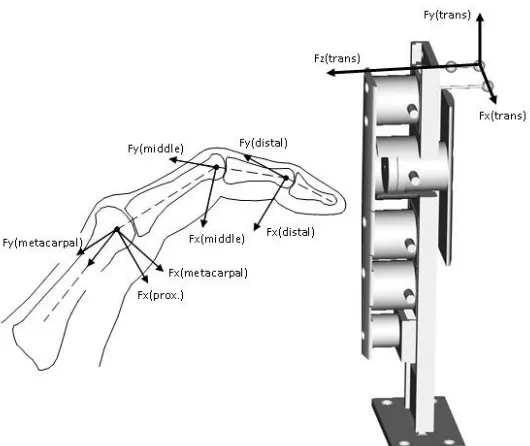
The joint coordinate systems used are illustrated in Figure 3. Table 2 details the overall

external loading effect at the digit tips in the transducer coordinate system. The forces

applied normal to the contact surface of the transducers were highest for the thumb,

averaging at 72.2 N. The average normal forces for the index, middle, ring and little

finger were 20 N, 25 N, 24 N and 11 N respectively. Table 3 details the external force

(14)

illustrated in Figure 3. The proximal force components for digits 2-5 were higher as a

percentage of the resultant force than the corresponding proximal force component for

the thumb. Higher percentage was seen in the dorsal component of the thumb than for the

other four digits. This was in agreement with the positioning of the fingers on the

gripping tool, where the distal interphalangeal joint angles were higher in digits 2-5 than

the thumb, resulting in the load being applied predominantly in the dorsal direction in the

thumb phalangeal coordinate system.

3.2 Metacarpophalangeal joint loads

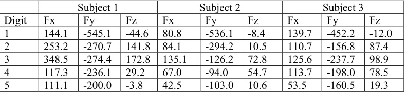
It can be seen in Table 4 that the proximal component of the metacarpophalangeal joint

contact force (Fy) was the highest, as a consequence of the tendon forces pulling the

bones together. From Table 4 it can be seen how the values differed from the external

loading, with the highest force-component acting proximally due to the contribution from

the tendons which were incorporated into the biomechanical model.

The resultant forces acting on the metacarpals were calculated by taking the quadratic

sum of the three force components for all the digits as:

Neutral position: 1836 N, 1232 N, 1350 N for subjects 1,2 and 3 respectively

Radial deviation: 1568 N, 1231 N, 976 N for subjects 1,2 and 3 respectively

(15)

3.3 Bone stress distribution

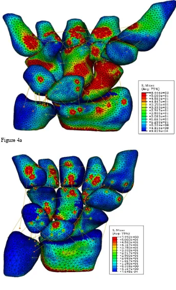
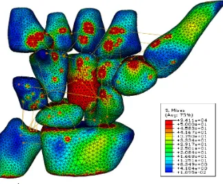
Surface stress contour plots can be seen in Figures 4a-c, for subjects 1, 2, and 3

respectively. It was observed that the stress distribution through the carpus was different

between subjects. Subject 1 showed high stresses down the radial aspect of the carpus, in

particular through the trapezium, trapezoid and the scaphoid. For subject 3 it could be

seen that the palmar side of the capitate was highly loaded which subsequently was

directed to the lunate. Subject 2 showed more concentrated stresses in the radius which

relieved the loading on the ulna. The stress density of the scaphoid is visibly the highest

for subject 1 (Figure 4a). By averaging the stress values for each of the 4 integration

points in the 10-node tetrahedral elements it was found that between 91.9% and 96.9% of

the elements had von Mises stresses below 50 MPa, with the vast majority of elements

below 20MPa with the wrist in a neutral position (Figure 5). The corresponding numbers

for radial deviation were 96.4% and 99.0% and for ulnar deviation 94.5% and 97.2%.

This was in agreement with the fact that the input loads were lower for the radially and

ulnarly deviated positions than for the neutral position. High stress intensity regions

could be seen at the insertion/origin points of the ligaments and in the surrounding

elements due to the coupling of the node points. These stresses were though highly

localized.

The strain values calculated for the cartilage on the radius were on average (standard

deviation) =-14.4% (27.0%) for the three subjects in a neutral position. The

corresponding value for the cortical bone was =-0.13% (0.56%) and for the cancellous

(16)

the cancellous region. Results in ulnar and radial deviation showed similar stress

distribution as in the neutral position with the majority of the loading travelling through

the radial aspect of the carpus.

3.4 Ligament forces

Table 5 shows the forces acting in a selected set of ligaments. The forces in the

radiotriquetral ligament ranged from 12.4 N to 74.4 N for all the models and were highest

in the neutral position averaging to 37.2 N, opposed to average values of 20.4 N and 19.7

N in radial and ulnar deviation respectively. Other ligaments that showed high activity

were the scaphotrapezoid band with average tension force of 147.3 N in a neutral

position, 152.1 N in radial deviation and 155.3 N in ulnar deviation. The

scaphotrapezium band averaged at 26.0 N in neutral position, 109.7 N in radial deviation

and 53.6 N in ulnar deviation. Less activity was seen in the scapholunate ligament which

averaged at 13.5 N in neutral position, 1.0 N in radial deviation and 8.2 in ulnar

deviation.

3.5 Forearm bone force transmission

Resultant reaction forces at the proximal end of the radius and ulna were calculated and

the load transfer ratio between the two bones estimated. Table 6 shows the load ratio

between the radius and ulna. Results showed that the load travelling through the radius

(17)

values ranged from 78.7% to 92.8% with the wrist in a neutral position. On average more

force was transmitted through the ulna during radial and ulnar deviation. This was

confirmed through a cadaveric study carried out at the University of Strathclyde,

Glasgow. Strain gauges were placed on the scaphoid, lunate, radius and ulna and strain

measurements taken with the wrist undergoing similar loading conditions as described

above. The results showed that on average 68% was transmitted through the radius and

32% through the ulna [33].

4 Discussion

4.1 Loading conditions

The joint contact values were reflective of the fact that the subjects were able to produce

the highest gripping force in neutral position and the lowest in ulnar deviation. The joint

contact forces ranged from 1.5-2.0 bodyweight between the subjects which might be

considered to be extremely high for a joint which is not a body weight bearing joint.

These force values were for maximal grip loading and so represent the maximum forces

that the subjects could apply. It would therefore be expected that the internal loading be

high in comparison with maximal possible (i.e. failure) loads. Subjects were only

required to maintain grip force of a few seconds duration. The joint contact force values

are thought to represent upper boundaries of the physiological loading. Other finite

(18)

4.2 Model construction

It was not possible to use automatic edge detecting procedures for automatic creation of

the models due to insufficient resolution of the MR scans. It was therefore necessary to

carry out edge detection manually. Great care was taken to recreate the anatomy as

accurately as possible. In order to check consistency of the geometrical construction, the

volume of the capitate bone was compared for the subjects for each position. It was found

that the deviation from the average value ranged between 3.6%-6.5% for subject 1,

0.2%-2.9% for subject 2 and 0.8% - 4.8% for subject 3 which showed that the repeatability of

the geometrical modelling was high. It was assumed therefore that the models

represented all of the bones with high geometrical accuracy.

4.3 Contact modelling

The contact between the bones was modelled so that once the bones had established

contact it was not possible for the bones to separate. This was necessary in order to

improve the stability of the carpus, particularly in the dorsal/palmar directions under the

influence of the shear forces.

4.4 Requirements for model convergence

The stability of the carpus is dependent on contributions from soft tissue structures,

mainly the ligaments and tendons. As the ligaments were modelled using

one-dimensional springs, the transverse stability generated by them in the wrist was not fully

included in the model. To overcome this limitation it was necessary to add constraints on

(19)

had been established. Modelling the transverse metacarpal ligaments as stiff did alter the

internal load distribution. However, this effect was predominantly in a medio-lateral

direction and the effects along the main loading axis were minimal.

To enhance convergence it was also necessary to prevent separation of the bones once

contact had been made. Attempts were made to use frictionless behaviour at the contacts

but this resulted in divergence where the bones became separated from each other. The

precautions put in place prevented dorsal/palmar instability and allowed model solution.

4.5 Stress of the carpal bones

Linearly elastic bone and cartilage material properties were used. The loading conditions

explored were of short duration and effectively static in the ‘hold’ phase of maximal grip

loading. It was therefore considered reasonable to ignore viscoeleastic effects. There has

been no attempt to include an exploration of the nonlinear aspect of bone and cartilage

behaviour. Inhomegeneity and anisotropy within the materials were not included.

Evaluation of inhomegeneity would to some extent be possible using statistical methods

with materials described using a distribution of properties. Anisotropic effects could be

included based on definitions of the radial and transverse directions within bones.

Exploration of the effects of these material properties on the stress distribution would

clearly be desirable, although this would add considerably to the computational solution

time and introduce further assumptions as accurate, local material property

(20)

From the stress distribution of the model it could be seen how the stress varied over the

carpal bones. The findings show similar results to the ones of Ulrich et al [34] who

reported that 93% of the elements were stressed between 0 and 30 MPa (von Mises

stresses) in a 3-bone model consisting of the radius, scaphoid and lunate. The

corresponding values based on the current model were 83.6%, 92.8% and 87.3% for

subjects 1, 2 and 3 respectively. The loading conditions of Ulrich et al's model consisted

of a total load of 1000N distributed between the scaphoid and lunate whereas the loading

conditions applied for the present model ranged from 1232 N to 1835N, so that the input

loads were higher, resulting in higher stress values. Another reason for the higher

percentage of elements loaded beyond 30 MPa was the fact that the ligament attachment

points showed high peak stresses which were distributed in the neighbouring elements

but died down rapidly after that. The application points of the loading onto the model also

exhibited high stress. These stress values were not thought to be representative of

physiological conditions.

The average strain values calculated for the cartilage, cancellous and cortical bone were

all within the physiological range. Bosisio et al. [35] presented ultimate strain values of

the cortical bone in the radius to be u=1.5 ± 0.1 % and the yield strain y=0.9 ± 0.2 % so

the strains presented in the current model were below the failure criteria. The cartilage

underwent higher values of strain and averaged at =-14.4% over the whole radiocarpal

joint. The failure strain value of cartilage under compression has been published by Kerin

et al. [36] to be 30%. For the 3 subjects in a neutral position it was found that on average

(21)

indicate that some of the cartilage could be damaged under such loading conditions or

that local imperfections in the model geometry caused unphysiological strain values.

4.6 Ligaments

The ligamentous contribution could be seen as localized stress increases but died out

rapidly and would have had minimal effect on the overall stress distribution at the joints.

This was due to the point to point connection of the ligaments in the model and was most

clearly seen in the transverse metacarpal ligaments which were modelled as stiff and thus

did not allow any extension. This was necessary as there were no other factors

contributing to the stabilization of the metacarpals within the model.

The palmar ligaments were in general more load bearing than the dorsal ligaments and

the results are in agreement with the theoretical model presented by Garcia-Elias in 1997

[37], where it was proposed that for gripping, the main stabilizing ligamentous structures

for the carpus are the scapho-trapezium-trapezoid ligaments, the scapho-triquetral

ligament and the radiotriquetral ligament. The radiotriquetral ligament showed high load

for all the subjects with the wrist in all positions. Less load was seen through the

scaphotriquetrum than expected due to Garcia-Elias' theory, but this transverse stability

was compensated elsewhere in the models, such as in the capitotrapezoid, capohamate

and hamotriquetrum ligaments.

4.7 Validation

Validation of finite element model results is critical to provide confidence that the

calculated load distributions are reasonable.

(22)

The relevance of subject specific anatomy to the outcomes of load distribution has been

demonstrated in the current study. It is therefore difficult to use the evidence from a

cadaveric study [33] on a wrist with a different anatomical configuration to directly

validate the current work. However, the cadaveric study results that were available

demonstrated general agreement with the outputs of this finite element study. The authors

are not aware of any reliable techniques that might be applied to subjects in vivo to assess

ligament loading and bone stress distributions without disrupting natural load transfer

characteristics. Further cadaveric work is desirable as maximal grip loading with

physiological load application has not been studied extensively.

5 Conclusions

The wrist model presented here offers major steps forward in the long process of creating

a physically representative numerical simulation of the wrist joint. This study

demonstrated how a geometrically accurate finite element model of a complex joint can

be constructed in a time efficient manner in order to be able to model anatomical

differences between subjects and to identify them as a part of a larger ensemble. This

gives the possibility of predicting load distributions following interventions in the wrist to

inform surgical planning. The differences observed in the load distribution in the wrist

joints studied, emphasises the need to move away from the idea of an ’average’ standard

(23)

6 Acknowledgements

The authors wish to thank Dr. N K Fowler for her input in the modelling, our subjects

and the Furlong Foundation and the Arthritic Research Campaign who funded this work.

7 References

1. McGrouther , D.A. and Higgins, P.O., Interactive Hand - Anatomy CD, Primal

Pictures, v.1.0

2. Palmer, A.K. and Werner, F.W., Biomechanics of the Distal Radioulnar Joint,

Clin. Orthop. Rel. Res, 1984, 187, 26–35.

3. Viegas, S.F., Tencer A.F., Cantrell, J., Chang, M., Clegg, P., Hicks, C.,

O’Meara, C., and Williamson, J.B., Load Transfer Characteristics of the Wrist:

Part 1, the Normal Joint, American Society for Surgery of the Hand, 1987,

12A(6), 971–978.

4. Viegas, S.F., Tencer, A.F., Cantrell, J., Chang, M., Clegg, P., Hicks, C.,

O’Meara, C., and Williamson, J.B., Load Transfer Characteristics of the

Wrist: Part 2, Perilunate Instability, American Society for Surgery of the Hand,

1987, 12A(6), 978–985.

5. Tencer, A.F., Viegas, S.F., Cantrell, J., Chang, M., Clegg, P., Hicks, C.,

O’Meara, C., and Williamson, J.B., Pressure distribution in the Wrist Joint,

Journal of Orthopaedic Research, 1988, 6(4), 509-517.

6. Schuind, F., Cooney, W.P., Linscheid, R.L., An K.N., and Chao, E.Y.S., Force

(24)

Two-Dimensional Study in the Posteroanterior Plane, Journal of Biomechanics,

1995, 28(5), 587-601.

7. Nedoma J. , Klézl Z., Fousek J., Kest ánek Z., Stehlík J, 2003, Numerical

Simulation of Some Biomechanical Problems, Mathematics and Computers in

Simulation, 61, 283-295

8. Carrigan, S.D., Whiteside, R.A., Pichora, D.R., and Small, C.F. Developement

of a Three Dimensional Finite Element Model for Carpal Load Transmission in

a Static Neutral Posture, Annals of Biomedical Engineering, 2003, 31, 718–

725.

9. Craigen, M.A.C. and Stanley, J.K., Wrist Kinematics: Row, Column or Both,

Journal of Hand Surgery (British and European Volume), 1995, 20B(2), 165–

170.

10. Fowler, N.K. and Nicol, A.C., Interphalangeal Joint and Tendon Forces:

Normal Model and Biomechanical Consequences of Surgical Reconstruction,

Journal of Biomechanics, 2000, 33, 1055-1062.

11. Fowler, N.K. and Nicol A.C., Functional and Biomechanical Assessment of the

Normal and Rheumatoid Hand, Clinical Biomechanics, 2001, 16(8), 660-666.

12. Rabai, G. and Vad, J., Validation of a Computational Fluid Dynamics Method

to be Applied to Linear Cascades of Twisted-Swept Blades, Periodica

Polytechnica Ser. Mech. Eng, 2005, 49(2), 163-180

13. Viceconti, M., Bellingeri L., Cristofolini, L., and Toni, A., A Comparative

Study on Different Methods of Automatic Mesh Generation of Human Femurs,

(25)

14. Rho, J.Y., Tsui, T.Y., and Pharr, G.M., Elastic properties of human cortical

and trabecular lamellar bone measured by nanoindentation, Biomaterials, 1997,

18(20), 1325-1330.

15. Kabel, J., Odaard, A., van Rietbergen, B. and Huiskes, R., Connectivity and the

elastic properties of cancellous bone, Bone, 1999, 24(2), 115-120.

16. Morgan, E.F., Bayraktar, H.H., Keaveny, T.M., Trabecular bone

modulus-density relationships depend on anatomic site. Journal of Biomechanics 36,

2003: 897–904

17. Berger, R.A., Imeada, T., Berglund, L., and An, K.N., Constraint and material

properties of the subregions of the scapholunate interosseous ligament., J Hand

Surg [Am], 1999,24(5), 953-62.

18. Bettinger, P.C., Linscheid, R.L., Berger, R.A., Cooney, W.P., and An, K.N.,

An Anatomic Study of the Stabilizing Ligaments of the Trapezium and

Trapeziometacarpal Joint, Journal of Hand Surgery,1999, 24(4), 786-798.

19. Bettinger, P.C., Smutz, W.P., Linscheid, R.L., Cooney, W.P., and An, K.N.,

Material Properties of the Trapezial and Trapeziometacarpal ligaments, Journal

of Hand Surgery, 2000, 25A, 1085-1095.

20. Cuénod, P., Charriére, E., and Papaloïzos, M. Y., A Mechanical Comparison of

Bone-Ligament-Bone Autografts From theWrist for Replacement of the

Scapholunate Ligament, Journal of Hand Surgery, 2002, 27A, 985-990.

21. Harvey, E. and Hanel, D., Bone-Ligament-Bone Reconstruction for

Scapholunate Disruption, Techniques in Hand and Upper Extremety Surgery,

(26)

22. Harvey, EJ, Hanel, D., Knight, J.B., and Tencer, A.F., Autograft replacements

for the scapholunate ligament: a biomechanical comparison of hand-based

autografts., J. Hand Surg [Am],1999, 24(5), 963-7.

23. Hofstede, D.J., Ritt, M.J., and Bos, K.E., Tarsal autografts for reconstruction of

the scapholunate interosseous ligament: a biomechanical study,1999, J Hand

Surg [Am], 24(5), 968-76

24. Johnston, J.D., Small, C.F., Bouxsein, M.L., and Pichora, D.R., Mechanical

Properties of the Scapholunate Ligament Correlate with Bone Mineral Density

Measurements of the Hand, Journal of Orthopaedic Research, 2004, 22,

867-871.

25. Logan, S.E. and Nowak, M.D., Distinguishing Biomechanical Properties and

Intrinsic and Extrinsic HumanWrist Ligaments, Journal of Biomechanical

Engineering, 1991,113(1), 85-93.

26. Lutz, M., Haid, C., Steinlechner, M., Kathrein, A., Arora, R., Fritz1, D., Gabl,

M., and Pechlaner, S., Scapholunate ligament reconstruction using a periosteal

flap of the iliac crest: a biomechanical study, Archives of Orthopaedic and

Trauma Surgery, 2004,124(4), 262-266.

27. Ritt, M.J., Berger, R.A., Bishop A.T., and An, K.N., The capitohamate

ligaments. A comparison of biomechanical properties., J Hand Surg [Br], 1996,

21(4),451-454.

28. Svoboda, S.J., Eglseder Jr, W.A., and Belkoff, S.M., Autografts from the foot

for reconstruction of the scapholunate interosseous ligament., J Hand Surg

(27)

29. Shin, S.S., Moore, D.C., McGovern, R.D., and Weiss, A.P., Scapholunate

ligament reconstruction using a bone-retinaculum-bone autograft: a

biomechanic and histologic study., J Hand Surg [Am], 1998, 23(2), 216-21.

30. Berger, R.A. and Garcia-Elias, M., Biomechanics of the Wrist Joint,

Springer-Verlag, NY, 1991, Chapter: General Anatomy of the Wrist, 1-22.

31. Horii, E., An, K.N., and Linscheid, R.L., Excursion of Prime Wrist Tendons,

Journal of Hand Surgery, 1993, 18A, 83-90.

32. Deakin, A. H., The Mechanical and Morphological Properties of Normal and

Rheumatoid Human Forearm Tendons, 2006, Ph.D. thesis, University of

Strathclyde.

33. Macleod, N.A., Nash D.H., Stansfield B.W., Bransby-Zachary M., Hems T..

Cadaveric Analysis of the Wrist and Forearm Load Distribution for Finite

Element Validation, Proceedings of the 6th International Hand and Wrist

Biomechanics Symposium, Tainan, Taiwan 2007, 11.

34. Ulrich, D., van Rietbergen, B., Laib, A., and Ruegsegger, P., Load Transfer

Analysis of the Distal Radius From In-vivo High Resolution CT-imaging,

Journal of Biomechanics, 1999, 32, 821-828.

35. Bosisio, M. , Talmant M. , Skalli, W., Laugier, P., and Mitton, D., Apparent

Young’s modulus of human radius using inverse finite-element method,

Journal of Biomechanics 40 (2007) 2022–2028

36. Kerin, A.J., Wisnom, M.R., and Adams, M.A., The compressive strength of

articular cartilage, Proceedings of the Institution of Mechanical Engineers, Part

(28)

37. Garcia-Elias, M., Kinetic Analysis of Carpal Stability During Grip, Hand

(29)

[image:29.612.121.471.88.276.2]

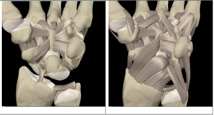
Figure 1: Palmar view of the wrist bones and the major ligaments

[image:29.612.81.364.324.531.2]

(30)

[image:30.612.87.352.62.285.2]

Figure 3: Coordinate systems used for the analysis of the gripping force and converting the externally measured loading into joint contact forces. Normal forces on the

transducers were directed in the direction. In the phalanx coordinate system, the z-direction was radial for the right hand, y-z-direction was proximal and x-z-direction was palmar.

(31)

[image:31.612.78.421.88.654.2]

(32)

Figure 4b

Figure 4c

[image:32.612.88.411.80.347.2]

(33)

[image:33.612.80.389.63.291.2]

Figure 5: Histogram showing the distribution of the von Mises stress values in the model elements. Values above 50 MPa are discarded from the histogram.

[image:33.612.89.379.337.561.2]

(34)

Young's modulus [MPa] Poisson's ratio Density [g/cm3]

Cartilage 10 0.4 1.1

Cancellous bone 100 0.25 1.3

Subchondral bone soft 1000 0.25 1.6

Subchondral bone hard 10000 0.2 1.8

[image:34.612.69.473.75.154.2]

Cortical 18000 0.2 2.0

Table 1: Material properties used in the model

Subject 1 Subject 2 Subject 3

Digit Fx Fy Fz Fx Fy Fz Fx Fy Fz

1 1.2 -12.3 99.0 10.2 -12.5 67.2 0.5 -6.0 50.6

2 1.0 -3.8 -14.2 -1.6 -5.9 -24.6 -0.5 -1.6 -22.5

3 8.3 -11.0 -41.0 -3.2 -0.4 -20.8 0.2 0.3 -13.5

4 -3.4 -10.4 -43.4 -4.1 0.6 -16.0 -2.4 0.8 -15.4

[image:34.612.71.473.191.281.2]

5 -2.5 -2.7 -16.7 -0.8 -2.8 -12.3 1.0 -1.1 -6.8

Table 2: External forces (Newtons) measured in the transducer coordinate system with the hand in a neutral position. The directions can be seen from Figure 3, with the Fz representing the normal force onto the force transducer, Fx and Fy represent the shear forces.

1 -98.0 11.9 -13.7 -51.0 18.0 -43.1 -46.9 5.6 -19.0

2 -2.5 -10.6 -9.9 -4.6 -18.1 -17.2 -1.7 -13.6 -17.9

3 -26.7 -32.6 -9.7 2.0 -15.9 -13.7 -1.0 -9.8 -9.2

4 -15.1 -41.1 -9.7 -4.1 -13.9 -7.9 -5.3 -13.8 -5.1

5 -5.3 -16.2 -0.2 -4.8 -11.3 -2.6 -4.0 -5.3 -2.3

Table 3: External forces (Newtons) measured in the metacarpal coordinate system with the hand in a neutral position. The directions can be seen from Figure 3. +ve Fx force is palmarly directed, +ve Fy is directed proximally and +ve Fz is radially directed

1 144.1 -545.1 -44.6 80.8 -536.1 -8.4 139.7 -452.2 -12.0

2 253.2 -270.7 141.8 84.1 -294.2 10.5 110.7 -156.8 87.4

3 348.5 -274.4 172.8 135.1 -126.2 72.8 125.6 -237.7 98.9

4 117.3 -236.1 29.2 67.0 -94.0 54.7 113.7 -198.0 78.5

5 111.1 -200.0 -3.8 42.5 -103.0 10.6 53.5 -160.5 19.3

[image:34.612.74.471.341.433.2] [image:34.612.76.472.491.582.2]

(35)

Neutral [N] Radial deviation [N] Ulnar deviation [N] 1 2 3 1 2 3 1 2 3

Radiotriquetral 74.4 22.6 14.5 15.5 19.6 26.1 12.4 20.5 27.0

Scaphotrapezoid 231.9 51.2 158.9 87.5 313.2 55.6 105.0 360.7 0

Scaphotrapezium 24.9 31.6 21.6 90.3 114.9 124.0 98.8 62.1 0

Scaphotriquetrum 0 0 4.5 0 0.4 1.9 0.2 2.7 0.9