On the validity of the ICFT
R
-matrix method: Fe
XIV
G. Del Zanna,
1‹N. R. Badnell,
2L. Fern´andez-Menchero,
2G. Y. Liang,
3H. E. Mason
1and P. J. Storey
41DAMTP, Centre for Mathematical Sciences, University of Cambridge, Wilberforce Road, Cambridge CB3 0WA, UK
2Department of Physics, University of Strathclyde, Glasgow G4 0NG, UK
3Key Laboratory of Optical Astronomy, National Astronomical Observatories, Chinese Academy of Sciences, 100012 Beijing, People’s Republic of China
4Department of Physics and Astronomy, University College London, London WC1E 6BT, UK
Accepted 2015 August 27. Received 2015 August 25; in original form 2015 July 22
A B S T R A C T
Recently, Aggarwal & Keenan published a DiracR-matrix (DARC) calculation for the electron-impact excitation of Fe XIV. A 136-level configuration-interaction/close-coupling (CI/CC) expansion was adopted. Comparisons with earlier calculations, obtained by Liang et al. with the intermediate coupling frame transformation (ICFT)R-matrix method, showed significant discrepancies. One of the main differences was that the Liang et al. effective collision strengths were consistently larger. Aggarwal & Keenan suggested various possible causes for the dif-ferences. We discuss them in detail here. We have carried out an ICFTR-matrix calculation with the same 136-level CI/CC expansion adopted by Aggarwal & Keenan, and compared the results with theirs and with those of Liang et al., which employed a much larger CI/CC expan-sion. We find that the main differences arise because of the different CC and CI expansions, and not because of the use of the ICFT method, as suggested by Aggarwal & Keenan. The significant increase in the effective collision strengths obtained by Liang et al. is mainly due to the extra resonances that are present because of the larger target expansion.
Key words: atomic data – techniques: spectroscopic.
1 I N T R O D U C T I O N
FeXIVis one of the most important iron ions for studies of the
solar corona (and in general for astrophysics). Aside from the fa-mous green coronal forbidden line in the visible spectrum, the strong FeXIVlines in the extreme ultraviolet are routinely used for plasma diagnostics, in particular to measure electron densities. Large discrepancies between observed and predicted line intensi-ties were present until Storey, Mason & Young (2000) resolved them with a new scattering calculation. Liang et al. (2010) have extended this work with a larger calculation. TheR-matrix suite of codes, described in Hummer et al. (1993) and Berrington, Eissner & Norrington (1995) were used by Liang et al. The calculation in the inner region was inLS coupling and included mass and Darwin relativistic energy corrections. The outer-region calculation used the intermediate coupling frame transformation (ICFT) method (Griffin, Badnell & Pindzola1998).
Aggarwal & Keenan (2014, hereafterAK14) recently carried out a new calculation for this ion using the Dirac AtomicR-matrix Code (DARC) of P. H. Norrington and I. P. Grant.AK14in their
paper were highly critical about the Liang et al. results in various respects, in particular about the thermally-averaged (effective) col-lisions strengthϒ(i− j). In their conclusions, they wrote: ‘The earlier calculations of Liang et al. (2010) appear to have
E-mail:[email protected]
mated the values ofϒfor almost all transitions and over an entire range of temperature.’
The authors suggested many possible explanations as to why the results were so different, the main one being the use of the ICFT
R-matrix approximation instead of the fully relativisticDARCone.
This criticism has subsequently been extended by the same authors (Aggarwal & Keenan2015) to similar ICFT calculations for all the ions in the Be-like sequence (Fern´andez-Menchero, Del Zanna & Badnell2014). They said: ‘it appears that the implementation of the ICFT approach, although computationally highly efficient, may not be completely robust.’
It was very surprising to seeAK14’s comments, if one considers three main issues. First, their results were based on a much smaller close-coupling (CC) expansion. For Fe XIV, the Liang et al. CC
expansion included the 197 lowest lying levels of the 16 config-urations: [1s22s22p6] 3sx3py3dz(x+y+z=3), 3s24l (l=s, p,
d, and f), and 3s 3p4l (l=s, p, d). On the other hand,AK14’s CC expansion included only the 136 fine-structure levels arising from the 12 lowest configurations: [1s22s22p6] 3s23p, 3s 3p2, 3s23d, 3p3,
3s 3p 3d, 3p23d, 3s 3d2, 3p 3d2, and 3s24l [l=s,p,d,f]. A larger
CC calculation giving uniformly largerϒ(i−j) with respect to a smaller CC calculation has the simple explanation of more resonant enhancement, especially for the higher lying states.
Secondly, for FeXIV, Liang et al. employed a much larger con-figuration interaction (CI) target expansion, including a further 77 configurations: 3s 3p 4f, 3p24l, 3p 3d 4l, 3d24l, 3l 4l 4l, and
2015 The Authors
at University of Strathclyde on March 18, 2016
http://mnras.oxfordjournals.org/
3l 3l (l = s, p, d, f, and g). The total CI included 2985 fine-structure levels. One would expect a better representation of the target with such a large expansion (as is indeed the case).
Thirdly, there is now a growing body of literature where the ICFT approach has been proven to be accurate. We start by noting that there is an extended literature where the results of the ICFT and full Breit–PauliR-matrix (BPRM) methods have been com-pared. For example, Griffin et al. (1998) compared the results of the ICFT and full BPRM methods for Mg-like ions, while Badnell & Griffin (1999) did the same for Ni V. More recently, Liang &
Badnell (2010) carried out extensive comparisons between ICFT andDARCfor FeXVIIand KrXXVII, while Liang, Whiteford &
Bad-nell (2009) made similar comparisons between ICFT andDARC(and
some BPRM) for FeXVI. Badnell & Ballance (2014) recently com-pared the results of ICFT, BPRM, andDARCon FeIII.
A detailed comparison of ICFT and BPRM calculations on the Be-like Al9+ has been presented in a separate paper
(Fern´andez-Menchero, Del Zanna & Badnell2015). As a test case, the results of a full BPRM calculation with an ICFT one were presented, using exactly the same structure (98-level CI/CC). Of all the tran-sitions (4753), only 1.7 per cent had effective collision strengths at peak ion abundance in equilibrium that differed by more than 10 per cent. These weak transitions have large uncertainties associ-ated with them.
In summary, no significant differences between the results of these methods have been found for these ions of nuclear charge up to nickel. The small differences that were found are within the typical spread seen in R-matrix calculations that use different CI and/or CC expansions, and resonance resolution. Indeed, when the exact same atomic structure is used to compare ICFT and BPRM, as it can be, then on using the exact same CC expansion the agree-ment between effective collision strengths is frequently better than 1 per cent. Physically, this is because the only difference between the ICFT and BPRM methods is the neglect of the spin–orbit in-teraction of the colliding electron with the ion by the former. This effect is far exceeded by the uncertainty due to the accuracy of the underlying atomic structure.
AK14refer to a problem that was encountered by Storey, Sochi & Badnell (2014) relating to deeply-closed channels in the outer-region ICFT calculation of O2+, when compared to a full Breit–Pauli
calculation, and suggested that this could be one of the causes of the discrepancies. However, Storey et al. (2014) note that such an issue only arises when resonance effective quantum numbers become small, and they provided a solution. The problem is peculiar to low-charge ions such as O2+and unusually small box sizes, and is
therefore not relevant to FeXIV. This is why the issue had not arisen before: all previous calculations used larger, often much larger, box sizes. Nevertheless, we have run new ICFT calculations (described below) with the original and the revised codes, and were satisfied to see only negligible differences.
AK14also mentioned a variety of other possible reasons for the discrepancies between theDARCand ICFT calculations for FeXIV.
Considering the importance of this ion, we discuss in what follows the various issues in some detail. Further detailed comparisons re-garding one of the Be-like ions, Al9+, are presented in a separate
paper (Fern´andez-Menchero et al.2015).
2 C O M PA R I S O N S
A proper comparison of scattering methods can only be carried out using the exact same atomic structure (not just the same CI expan-sion but the same orbitals and same operators). As we mentioned
in the Introduction, such detailed comparisons have already been provided for other ions – see, in particular, Fern´andez-Menchero et al. (2015).
For the purpose of this paper, we have carried out an ICFT cal-culation that was as close as possible to theAK14one, with the same 136-level CC/CI expansion, so we could compare this to the larger 197/2895-level calculation presented by Liang et al., using the same methods and codes.
We have also examined the convergence of the CC expansion of Liang et al. by extending it from 197 to 228 levels, using the exact same structure. We find no important differences and so, to avoid confusion, we report this in an appendix.
2.1 Atomic structure – CI effects
For the atomic structureAK14used the GRASP(General-purpose
Relativistic Atomic Structure Package) code, originally developed by Grant et al. (1980) and then revised by P. H. Norrington.AK14 performed three sets of atomic structure calculations: GRASP1a, GRASP1b, and GRASP2. GRASP1a adopted the 136-levels target previously mentioned and is associated with the scattering calcula-tion. With GRASP1b the Breit and quantum electrodynamics effect corrections were added, while GRASP2 was a different calculation with additional CI, for a total of 332 levels.
We used the AUTOSTRUCTURE program (Badnell 2011) and
in-cluded the same set of configurations adopted by AK14, giving rise to 60LSterms and 136 fine-structure levels. We constructed the target wavefunctions using radial wavefunctions calculated in a scaled Thomas–Fermi–Dirac–Amaldi statistical model potential. A weighted-sum of all the eigenenergies was minimized to determine the optimum structure by varying a set of scaling parameters. The results were: 1s:1.405 43, 2s:1.106 83, 2p:1.052 05, 3s:1.118 81, 3p:1.078 45, 3d: 1.107 04, 4s: 1.148 74, 4p:1.095 23, 4d:1.121 99, 4f:1.283 80.
The target energies are relatively close to theAK14GRASP1a energies, as shown in TableA1in the appendix. As also noted by AK14, the Liang et al. energies are generally in better agreement with the observed energies, hence the Liang et al. CI expansion is more accurate. This is expected, given the much larger set of configurations included (we recall 2985 fine-structure levels versus 136).
In terms of level energies, AK14also noted that: ‘Differences with the NIST compilations are generally smaller, but are up to 1.4 per cent for some levels, such as 3s24p2Po
1/2,3/2, for which our
GRASP1b energies agree better with the measurements.’ Regarding the 3s24p2Po
1/2,3/2levels, we note that theAK14GRASP2 energies
are actually closer to the Liang et al. energies than those of the GRASP1 calculations. In other words, increasing CI provides en-ergies that are increasingly different than the National Institute of Standards and Technology (NIST)1ones for the 3s24p. There is,
however, a more important point; that the NIST energies for these levels are incorrect, as discussed in Del Zanna (2012). The two main decays from the 3s24p2P
1/2, 3/2levels were identified from
laboratory plates by Fawcett et al. (1972) at 91.273 and 91.009 Å, respectively. Del Zanna (2012) used the Liang et al. calculations to predict that the first transition should be the third strongest FeXIV
soft X-ray line. However, there is no such strong emission line in the solar spectra. The only solar spectral line that matches the predicted intensity is the previously unidentified line observed by Manson
1http://www.nist.gov
at University of Strathclyde on March 18, 2016
http://mnras.oxfordjournals.org/
(1972) at 93.61 Å. Del Zanna (2012) identified several other strong soft X-ray lines using both solar spectra and the original laboratory plates used by Fawcett for his identification work. The 93.61 Å line is also observed in Fawcett’s laboratory plate C53 at exactly the same wavelength. Manson (1972) showed that this line becomes enhanced in active Sun conditions, which indicates that the line must be produced in active region cores (2–3 MK), which is an-other argument in favour of the identification as FeXIV. The other
decays from the 3s24p2P
1/2, 3/2levels were also identified in Del
Zanna (2012). The corresponding observed energies of these levels are in very good agreement with the Liang et al. ab initio energies, contrary to what is stated byAK14.
In terms of transition probabilities,AK14compared the A-values for the E1 transitions within the (energetically) lowest 15 levels, which produce the most important lines for this ion.AK14stated: ‘Our GRASP1 A-values agree within 10 per cent with those of Liang et al. for almost all transitions, the only exceptions being a few weak transitions, such as 8–15 (f∼105) and 12–15 (f∼106).’AK14
correctly noted that large discrepancies for very weak transitions are common, because such lines can be sensitive to the differing amount of CI included in the calculations.
Such CI effects become more prominent for the higher levels, as one would expect. We have considered thegf-values for all the dipole-allowed transitions from the ground configuration, and com-pared the results of the presentAUTOSTRUCTURE136-level calculation
with theAK14(using their published line strengths) and the Liang et al. ones. As shown in Fig.1(top), there is overall good agree-ment (within 20–30 per cent) between the presentAUTOSTRUCTURE
136-level calculation and theGRASP136-level calculation ofAK14.
Therefore, one would expect that also the corresponding collision strengths would have a similar agreement, as indeed is the case, as shown below.
However, as Fig.1(bottom) shows, there are a number of cases where thegf-values of the presentAUTOSTRUCTURE136-level calcu-lation differ significantly from those of the Liang et al. calcucalcu-lation. They mainly occur for the higher levels, and show the significant effect of a different CI expansion. We note that differences for tran-sitions within the lowest 12 levels are at most 2–3 per cent, i.e. CI uncertainties are negligible for these low-lying levels.
2.2 Collision strengths
TheR-matrix method that we used in the inner region of the scatter-ing calculation is described in Hummer et al. (1993) and Berrington et al. (1995). We performed the calculation inLS coupling and included the mass–velocity and Darwin relativistic operators. The outer region calculation used the ICFT method (Griffin et al.1998). The expansion of each scattered electron partial wave was carried out over a basis set of 30 functions within theR-matrix boundary, as inAK14. We note that Liang et al. used a basis set of 40 continuum functions.
We included exchange in the inner region corresponding to a total angular momentum quantum numberJ=14. We have supplemented the exchange contributions with a non-exchange calculation to cover
J=15–38.
[image:3.595.308.548.54.401.2]Dipole-allowed transitions were topped-up to infinite partial wave using an intermediate coupling version of the Coulomb–Bethe method as described by Burgess (1974) while non-dipole allowed transitions were topped-up assuming that the collision strengths form a geometric progression inJ(see Badnell & Griffin2001).
Figure 1. Oscillator strengths (gf-values) for all transitions from the ground configuration as calculated with the present CI (136 levels) versus those calculated byAK14(top) and with the much larger CI (2985 levels) by Liang et al. (bottom). The dashed lines indicate±20 per cent.
The outer region calculation was performed in a number of stages. A coarse energy mesh was chosen at all energies forJ=15–38 and above all resonances forJ=0–14, up to 260 Ryd, which is the same maximum energy used byAK14. The resonance region was calculated with an increasing number of points, up to 16 000, equivalent to a constant energy resolution of 0.001 Ryd.
The collision strengths were extended to high energies by inter-polation using the appropriate high-energy limits in the Burgess & Tully (1992) scaled domain. The high-energy limits were calcu-lated withAUTOSTRUCTUREfor both optically-allowed (see Burgess,
Chidichimo & Tully1997) and non-dipole allowed transitions (see Chidichimo, Badnell & Tully 2003). The temperature-dependent effective collisions strengthϒ(i−j) were calculated by assuming a Maxwellian electron distribution and linear integration with the final energy of the colliding electron.
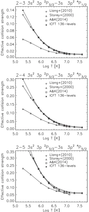
In terms of collisions strengths,AK14noted very good agreement at 30 Ryd between their results and the Storey et al. (2000), except for the 2–3, 2–4, and 2–5 transitions. We note that for astrophys-ical applications the important quantity is the effective collisions strength. As Fig.2shows, there is very good agreement between theAK14and Liang et al. calculations, while the Storey et al. (2000) are progressively lower at lower temperatures (as discussed in Liang et al.).
AK14 also noted some differences in the effective colli-sions strengths for the forbidden transition within the ground
at University of Strathclyde on March 18, 2016
http://mnras.oxfordjournals.org/
Figure 2. Thermally-averaged collision strengths for a selection of transi-tions (see text) as calculated with the present CI/CC of 136 levels, compared to those calculated by Liang et al. (2010, Liang+(2010)), Storey et al. (2000, Storey+(2000)), and Aggarwal & Keenan (2014, A&K 2014).
configuration, with the Liang et al. values being higher than those ofAK14. We note that there is actually an excellent agreement at all high temperatures, with discrepancies present only at very low temperatures (100 000 K and below). Such discrepancies are com-mon, and normally depend on the position of the resonances near threshold.
Finally,AK14stated: ‘We believe the values ofϒcalculated by Liang et al. are overestimated for almost all transitions and at all temperatures. Hence, a re-examination of their results is desirable.’ We note, however, that the same authors point out in their table 8 that the two calculations generally agree to within 20 per cent for the transitions within the lowest 10 levels, at the temperature of maximum ion abundance (2 MK) in equilibrium.
AK14stated that for about half the transitions there are differ-ences of over 20 per cent, and their [Liang et al.] results are mostly higher. However, no comparisons were shown. We have therefore produced such comparisons. We note that for many levels the en-ergy ordering of the two calculations is different. We also note that
the population of the levels for astrophysical plasmas is driven by excitations from the ground configuration, so we focus our atten-tion on these transiatten-tions. We have split up the transiatten-tions into three groups. The first group includes the excitations to the 3s23p, 3s 3p2,
3s23d, 3p3, 3s 3p 3d, and 3p23d. Such levels produce the strongest
lines for this ion. The second group includes the excitations from the ground configuration to the 3s 3d2and 3p 3d2, which are less
important, while the third group those to the 3s24l [l=p,d,f] levels.
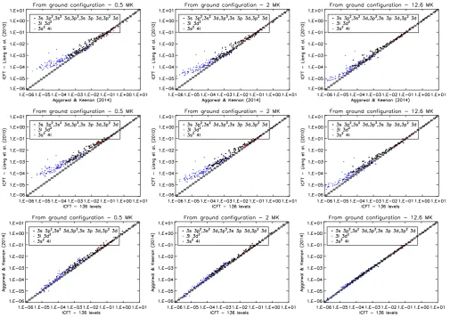
We note thatAK14only provided effective collision strengths for temperatures higher than logT[K]=5.7, so we show in Fig.3 (top row) a comparison at this lower temperature, as well as at the temperature of maximum abundance (2 MK) and at a high temperature (12 MK) with the Liang et al. data. The dashed lines show+/−20 per cent. For the lower levels there is good agreement (within 20 per cent) at all temperatures, while for the upper ones we clearly see a tendency for the Liang et al. values to be larger for weaker transitions.
Fig.3(middle row) shows the comparisons between our ICFT 136-level calculation (0.001 Ryd energy resolution, ab initio ener-gies, see below) and the Liang et al. data. There are clear striking similarities. The scatter in the points is mainly caused by the dif-ferent CI expansion, while the fact that the Liang et al. values are consistently larger at lower temperatures has its simplest explana-tion in the well-known fact that a larger CC expansion generates more resonances which increasingly enhances the transitions to higher states of the smaller calculation. Indeed, such an effect is intrinsic to allR-matrix scattering calculations, be they LS, ICFT, BPRM, orDARC– Fern´andez-Menchero et al. (2015) demonstrate
this explicitly for Be-like Al9+. Thus, we find no evidence to support
the conjecture ofAK14that the ICFT method is not ‘robust’. To further confirm the fact that the ICFT andDARCcalculations produce similar effective collision strengths, we show in Fig. 3 (bottom row) a comparison between our 136-level CI/CC ICFT (0.001 Ryd energy resolution, ab initio energies) results and the AK14ones. There are no obvious trends, although theAK14ones tend to be slightly larger, especially for the weaker transitions.
Finally, in the Appendix we look at expanding the 197-level CC expansion to 228 levels. We find little further resonance enhance-ment.
2.2.1 Sensitivity to the energy resolution
The energy resolution that is adopted within the resonance region can have some effects on the collision strengths.
AK14have calculatedin (most of) the thresholds region in a narrow energy mesh of 0.001 Ryd, although a mesh of 0.002 Ryd has also been used whenever the energy difference between any two thresholds is wider, such as levels 2 and 3. In totalhave been calculated at over 10 500 energies.
If we look at the GRASP1a level energies in table 1 ofAK14we note only three level pairs (26–27, 58–59 and 106–107) separated by less than 0.002 Ryd, viz. by 0.000 95, 0.000 69, and 0.001 69 Ryd. These excepted the energy mesh quoted byAK14is coarser than the one used by Liang et al., where a fixed resolution of 0.001 69 Ryd was adopted.
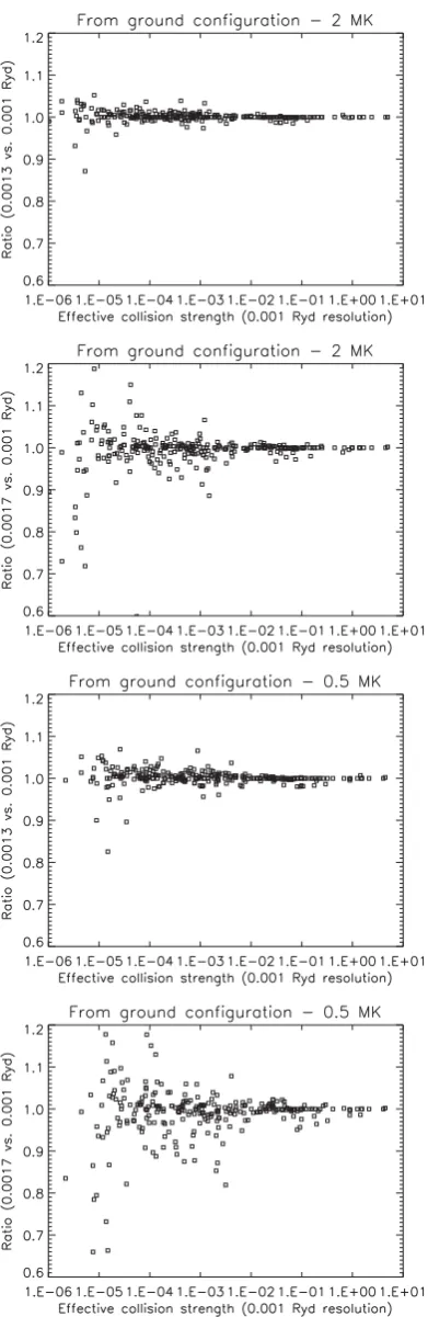
We have calculated three sets of effective collision strengths with increasing resolution, to assess how this affects the results. One calculation had only 9600 points in the resonance region (equivalent to 0.001 73 Ryd), one had 12 800 points (equivalent to 0.0013 Ryd), and the third one had 16 000 points (equivalent to 0.0010 Ryd).
Fig.4shows the ratios in the effective collision strengths between the two lower resolution calculations and the highest one, for all
at University of Strathclyde on March 18, 2016
http://mnras.oxfordjournals.org/
Figure 3. Thermally-averaged collision strengthsϒfor transitions from the ground configuration 3s23p levels at three different temperatures. Top row:AK14
results versus Liang et al. (2010). Middle row: the present 136-levels (60LSterms) ICFT calculation versus Liang et al. (2010). Bottom row: the present 136-levels ICFT calculation versusAK14. The dashed lines indicate±20 per cent.
the transitions between the ground configuration and the excited states. Except for a few weak transitions, at 2 MK the effective collision strengths obtained with 0.0013 Ryd resolution agree within 5 per cent with those obtained with the 0.0010 Ryd resolution, while for the calculation with 0.001 73 Ryd resolution the scatter is larger, but still within±10 per cent, except a few amongst the weakest transitions. At 0.5 MK, the scatter is larger but still well within 20 per cent for most transitions. The scatter is much reduced at higher temperatures as one would expect. This indicates that only a small amount (at most 10 per cent) of the differences between theAK14and the Liang et al. effective collision strengths can in principle be ascribed to the different energy resolution; the rest then is due to the increased resonance enhancement and/or differences in atomic structure. Indeed the differences in the atomic structure produce typically larger effects than the energy resolution, as also discussed in Fern´andez-Menchero et al. (2015).
2.2.2 Sensitivity to the threshold level energy position
Within the outer region calculations, it is possible to set the threshold level energies to the observed values, in order to better position the resonances at the correct energies. The differences between observed and ab initio level energies are not large, but it is interesting to see what effect this has on the collision strengths. Presumably,
AK14used the GRASP1a energies. Liang et al. used instead the observed energies (whenever available) to position the resonances. We have first obtained a set of ‘best guess’ energies by linearly interpolating the ab initio energies with the known observed en-ergies. We have used these best guess energies whenever observed energies were not available. We have then run the outer region ICFT calculation with the highest number of points in the resonance re-gion (16 000), and recalculated the effective collision strengths. Fig.5shows the comparison in the effective collision strengths, for 0.5 MK. Variations of the order of 20 per cent or so are present for the weaker transitions, while of course variations tend to increase for even lower temperatures.
3 C O N C L U S I O N S
We have considered in detail all the various potential causes sug-gested byAK14as a possible explanation for the discrepancies in the effective collision strengths obtained with theirDARC
calcula-tion and the Liang et al. (2010) ICFT calculations for FeXIV. We
have found that the main differences arise because of the different CC and CI expansions. Indeed, an ICFT calculation with the same CC and CI expansion as adopted by Aggarwal & Keenan (2015) produces very similar results to theirs. The significant increase in the effective collision strengths obtained by Liang et al. (2010) is
at University of Strathclyde on March 18, 2016
http://mnras.oxfordjournals.org/
Figure 4. Ratios in the effective collision strengths between the two lower resolution calculations (0.0013 and 0.0017) and the highest one (0.0010), at 2 and 0.5 MK.
Figure 5. A comparison of the effective collision strengths obtained with the 136-level ICFT, only changing the threshold positions to the observed or best guess energies, for 0.5 MK.
mainly due to the extra resonances that are present because of the larger CC expansion.
The fact that the Liang et al. (2010) calculations have a more ac-curate CI expansion and extra resonances means that their approach is still to date the best for this ion. In the appendix we detailed a modest improvement which can be made to them.
The energy resolution and the threshold position do have some effects on the final collision strengths, but are of relatively minor importance, compared to the CI and CC effects.
Similar conclusions were obtained on the Be-like Al9+
(Fern´andez-Menchero et al.2015). There, ICFT and Breit–Pauli
R-matrix calculations with the same target (98-levels) were shown to agree very closely, confirming that the ICFT approach is robust. TheDARC98-levels calculations of Aggarwal & Keenan (2015) for Al9+were found to be less accurate than the 238-level ICFT
cal-culation of Fern´andez-Menchero et al. (2014). The same issues obviously apply to the other ions in the Be-like sequence and, as we have just seen, ions of other sequences.
We have demonstrated that the ICFT calculations are robust and that the main difference between the ICFT andDARCcalculations
lies in the choice of the CI/CC expansions.
AC K N OW L E D G E M E N T S
This work was funded by STFC (UK) through the University of Cambridge DAMTP astrophysics grant and the University of Strath-clyde UK APAP network grant ST/J000892/1. GYL acknowledges the support from the National Natural Science Foundation of China under grant C: 11273032.
R E F E R E N C E S
Aggarwal K. M., Keenan F. P., 2014, MNRAS, 445, 2015 (AK14) Aggarwal K. M., Keenan F. P., 2015, MNRAS, 447, 3849 Badnell N. R., 2011, Comput. Phys. Commun., 182, 1528 Badnell N. R., Ballance C. P., 2014, ApJ, 785, 99
Badnell N. R., Griffin D. C., 1999, J. Phys. B: At. Mol. Phys., 32, 2267 Badnell N. R., Griffin D. C., 2001, J. Phys. B: At. Mol. Phys., 34, 681 Berrington K. A., Eissner W. B., Norrington P. H., 1995, Comput. Phys.
Commun., 92, 290
Burgess A., 1974, J. Phys. B: At. Mol. Phys., 7, L364 Burgess A., Tully J. A., 1992, A&A, 254, 436
at University of Strathclyde on March 18, 2016
http://mnras.oxfordjournals.org/
Burgess A., Chidichimo M. C., Tully J. A., 1997, J. Phys. B: At. Mol. Phys., 30, 33
Chidichimo M. C., Badnell N. R., Tully J. A., 2003, A&A, 401, 1177 Del Zanna G., 2012, A&A, 546, A97
Fawcett B. C., Kononov E. Y., Hayes R. W., Cowan R. D., 1972, J. Phys. B: At. Mol. Phys., 5, 1255
Fern´andez-Menchero L., Del Zanna G., Badnell N. R., 2014, A&A, 566, A104
Fern´andez-Menchero L., Del Zanna G., Badnell N. R., 2015, MNRAS, 450, 4174
Grant I. P., McKenzie B. J., Norrington P. H., Mayers D. F., Pyper N. C., 1980, Comput. Phys. Commun., 21, 207
Griffin D. C., Badnell N. R., Pindzola M. S., 1998, J. Phys. B: At. Mol. Phys., 31, 3713
Hummer D. G., Berrington K. A., Eissner W., Pradhan A. K., Saraph H. E., Tully J. A., 1993, A&A, 279, 298
Liang G. Y., Badnell N. R., 2010, A&A, 518, A64
Liang G. Y., Whiteford A. D., Badnell N. R., 2009, A&A, 500, 1263 Liang G. Y., Badnell N. R., Crespo L´opez-Urrutia J. R., Baumann T. M.,
Del Zanna G., Storey P. J., Tawara H., Ullrich J., 2010, ApJS, 190, 322 Manson J. E., 1972, Sol. Phys., 27, 107
Storey P. J., Mason H. E., Young P. R., 2000, A&AS, 141, 285 Storey P. J., Sochi T., Badnell N. R., 2014, MNRAS, 441, 3028
A P P E N D I X A : E N E R G I E S
[image:7.595.74.521.267.645.2]TableA1provides a comparison of target level energies.
Table A1. A comparison of target level energies. Only a selection of levels is shown. Energies are in kaysers.Eexp: experimental values; Epresent: present 136-levelAUTOSTRUCTURE(AS) calculation;EL10: Liang et al. (2010)AUTOSTRUCTURE(AS) calculation;EAK14: Aggarwal &
Keenan (2014) GRASP1a calculation. The values in brackets are the differences with the experimental values.
i Conf. Mixing LSJ Eexp Epresent EL10 EAK14
(%) AS AS GRASP1a
1 3s23p (96) 2P
1/2 0.0 0.0 0.0 (0) 0.0 (0)
2 3s23p (96) 2P
3/2 18 852.0 18 455.0 (397) 18 332.0 (520) 19 242.0 (−390)
3 3s 3p2 (98) 4P
1/2 225 114.0 223 262.0 (1852) 221 637.0 (3477) 223 024.0 (2090)
4 3s 3p2 (99) 4P
3/2 232 789.0 230 520.0 (2269) 229 073.0 (3716) 230 854.0 (1935)
5 3s 3p2 (97) 4P
5/2 242 387.0 239 853.0 (2534) 238 615.0 (3772) 240 799.0 (1588)
6 3s 3p2 (86) +11(c3 11) 2D
3/2 299 242.0 300 206.0 (−964) 298 460.0 (782) 301 007.0 (−1765)
7 3s 3p2 (85) +12(c3 11) 2D
5/2 301 469.0 302 191.0 (−722) 300 591.0 (878) 303 335.0 (−1866)
8 3s 3p2 (79) +9(17) 2S
1/2 364 693.0 368 733.0 (−4040) 367 611.0 (−2918) 370 670.0 (−5977)
9 3s 3p2 (78) +8(18) 2P
1/2 388 510.0 393 089.0 (−4579) 392 054.0 (−3544) 395 757.0 (−7247)
10 3s 3p2 (95) 2P
3/2 396 512.0 401 182.0 (−4670) 400 255.0 (−3743) 404 227.0 (−7715)
11 3s23d (85) +6(c2 11) 2D3/2 473 223.0 482 495.0 (−9272) 480 239.0 (−7016) 483 639.0 (−10416)
12 3s23d (85) +7(c2 11) 2D5/2 475 202.0 484 993.0 (−9791) 482 630.0 (−7428) 485 718.0 (−10516)
13 3p3 (64) +29(c5 28) 2D3/2 576 383.0 576 009.0 (374) 574 615.0 (1768) 577 319.0 (−936)
14 3p3 (68) +30(c5 30) 2D5/2 580 233.0 579 524.0 (709) 578 210.0 (2023) 581 118.0 (−885)
15 3p3 (93) 4S
3/2 589 002.0 589 106.0 (−104) 588 402.0 (600) 592 015.0 (−3013)
16 3s 3p 3d (96) 4F
3/2 – 644 069.0 642 341.0 643 192.0
17 3p3 (80) +34(c5 12) 2P
1/2 642 179.0 644 879.0 (−2700) 643 661.0 (−1482) 647 917.0 (−5738)
18 3s 3p 3d (98) 4F
5/2 645 988.0 648 108.0 (−2120) 646 434.0 (−446) 647 435.0 (−1447)
19 3p3 (71) +33(c5 12) 2P
3/2 645 409.0 647 801.0 (−2392) 646 782.0 (−1373) 651 305.0 (−5896)
20 3s 3p 3d (98) 4F
7/2 651 946.0 653 913.0 (−1967) 652 337.0 (−391) 653 604.0 (−1658)
21 3s 3p 3d (99) 4F
9/2 660 263.0 661 913.0 (−1650) 660 492.0 (−229) 662 178.0 (−1915)
22 3s 3p 3d (69) +28(25) 4P
5/2 690 304.0 694 279.0 (−3975) 693 115.0 (−2811) 694 157.0 (−3853)
23 3s 3p 3d (54) +26(43) 4D
3/2 692 662.0 696 509.0 (−3847) 695 339.0 (−2677) 696 808.0 (−4146)
24 3s 3p 3d (83) +25(15) 4D
1/2 694 168.0 698 059.0 (−3891) 696 838.0 (−2670) 698 628.0 (−4460)
25 3s 3p 3d (84) +24(15) 4P
1/2 703 750.0 706 287.0 (−2537) 705 555.0 (−1805) 707 429.0 (−3679)
26 3s 3p 3d (55) +23(43) 4P
3/2 704 209.0 707 171.0 (−2962) 706 311.0 (−2102) 708 296.0 (−4087)
27 3s 3p 3d (98) 4D
7/2 703 393.0 707 575.0 (−4182) 706 383.0 (−2990) 708 400.0 (−5007)
28 3s 3p 3d (73) +22(24) 4D
5/2 704 114.0 707 677.0 (−3563) 706 660.0 (−2546) 708 735.0 (−4621)
29 3s 3p 3d (50) +13(c4 17) +38(27)
2D
3/2 717 195.0 722 539.0 (−5344) 721 362.0 (−4167) 724 165.0 (−6970)
30 3s 3p 3d (48) +14(c4 15) +40(26) +22(5)
2D
5/2 717 861.0 723 178.0 (−5317) 722 024.0 (−4163) 724 796.0 (−6935)
31 3s 3p 3d (64) +36(32) 2F
5/2 744 965.0 754 236.0 (−9271) 751 525.0 (−6560) 755 392.0 (−10 427)
32 3s 3p 3d (65) +35(33) 2F
7/2 759 814.0 768 529.0 (−8715) 766 012.0 (−6198) 770 691.0 (−10 877)
at University of Strathclyde on March 18, 2016
http://mnras.oxfordjournals.org/
Table A1 – continued
i Conf. Mixing LSJ Eexp Epresent EL10 EAK14
(%) AS AS GRASP1a
33 3s 3p 3d (78) +18(c4 14) 2P
3/2 807 113.0 818 431.0 (−11 318) 816 798.0 (−9685) 821 603.0 (−14 490)
34 3s 3p 3d (86) +17(c4 12) 2P
1/2 815 125.0 826 433.0 (−11 308) 824 734.0 (−9609) 829 932.0 (−14 807)
35 3s 3p 3d (63) +32(33) 2F
7/2 817 593.0 829 852.0 (−12 259) 828 236.0 (−10643) 832 277.0 (−14 684)
36 3s 3p 3d (64) +31(32) 2F
5/2 820 601.0 832 512.0 (−11 911) 830 929.0 (−10328) 835 286.0 (−14 685)
37 3s 3p 3d (90) 2P
1/2 839 492.0 853 924.0 (−14 432) 850 266.0 (−10774) 857 100.0 (−17 608)
38 3s 3p 3d (54) +13(c4 10) +29(12) +33(6)
+39(12)
2D
3/2 840 775.0 854 940.0 (−14 165) 852 103.0 (−11328) 858 274.0 (−17 499)
39 3s 3p 3d (77) +38(8) 2P3/2 843 656.0 858 109.0 (−14 453) 854 724.0 (−11068) 861 270.0 (−17 614)
40 3s 3p 3d (66) +14(c4 12) +30(16)
2D
5/2 844 477.0 858 124.0 (−13 647) 855 809.0 (−11332) 861 757.0 (−17 280)
101 3s24s (99) 2S
1/2 1435 020.0 145 7991.0 (−22 971) 1435 636.0 (−616) 1454 621.0 (−19 601)
122 3s24p (99) 2P
1/2 1541 394.0 1575 008.0 (−33 614) 1544 514.0 (−3120) 1570 660.0 (−29 266)
125 3s24p (99) 2P
3/2 1548 163.0 1581 536.0 (−33 373) 1552 087.0 (−3924) 1577 784.0 (−29 621)
137 3s24d (99) 2D
3/2 1695 980.0 1729 627.0 (−33 647) 1700 712.0 (−4732) 1725 557.0 (−29 577)
138 3s24d (99) 2D
5/2 1697 290.0 1730 812.0 (−33 522) 1702 176.0 (−4886) 1726 699.0 (−29 409)
146 3s24f (99) 2F
5/2 1788 640.0 1819 597.0 (−30 957) 1795 250.0 (−6610) 1814 556.0 (−25 916)
148 3s24f (99) 2F
7/2 1788 380.0 1819 966.0 (−31 586) 1795 665.0 (−7285) 1814 887.0 (−26 507) Note.The indexingifollows Liang et al. (2010).
A P P E N D I X B : C C C O N V E R G E N C E
The 16 CC configurations used by Liang et al., and listed in the Introduction, give rise to 89 terms and 203 levels. The highest six levels lie above the lowest CI ones and so results (andϒ) were restricted to the lowest 197.
A 98 termLS-couplingR-matrix calculation was carried out by Liang et al. so as to span all terms of the first 16 configurations, and so a few ‘CI’ terms were actually included in theLSCC expansion. These 98 terms give rise to 228 levels, but only the lowest 197 were retained in the final ICFT recoupling, i.e. resonances are attached to just 197 levels. We have rerun the final recoupling calculation retaining all 228 levels, and thus generating resonances attached to 228 levels. While transitions to these higher levels themselves are more uncertain, hence the original restriction, the additional resonances they generate enable us to examine the sensitivity of lower transitions to further resonance enhancement.
In addition, we found that recoupling just the 197-levels of the
K-matrix to convert to theS-matrix, as done by Liang et al, gave rise to small pseudo-resonance-like features at energies above all channels open for some transitions, particularly high-lying ones. These disappear on converting the fullK-matrix to theS-matrix, either by recoupling the full 228-level K-matrix or by convert-ing the full 98 termK-matrix to the (LS)S-matrix and recoupling it, either retaining 197- or 228-levels. The final result via either route is essentially identical. The results of the 228-levels calcu-lation will be made available via our UK APAP network website (www.apap-network.org).
In Fig.B1we compare the present 228 CC effective collision strengths with the 197 CC ones of Liang et al. at the temperature of peak abundance (2 MK) for transitions from the levels of the ground configuration to the lowest 136-levels, as compared previously in Fig.3. The very weakest transitions show a small reduction while there is little systematic further resonance enhancement. The spread is negligible compared to that seen in Fig.3.
[image:8.595.310.536.319.476.2]Next, to show the effects we have seen in Fig.3onϒ of the 136- versus 197-level CC expansion on the underlying collision strengths, we have selected as an example two transitions that
Figure B1. A comparison of the effective collision strengths calculated by Liang et al. (2010) with the 197-level CC expansion with those we have obtained with a 228-level CC expansion, at peak ion abundance (2 MK).
have similar high-energy limits but significantly increased collision strengths with the larger CC expansion.
The first is a weak dipole-allowed transition (1–82), with a small
gf=0.001 32 in the 136-level CI/CC ICFT calculation, and a sim-ilar one (gf=0.001 33) in the Liang et al. ICFT larger calculation. Fig.B2(bottom) shows that the larger calculation produces a sig-nificant enhancement in the effective collision strengths, by a factor of 1.6 at 2 MK, increasing towards low temperatures. The two top plots show the collision strengths in the scaled Burgess & Tully (1992) domain, where the last point is the scaled high-energy limit. The second is a Born-allowed transition (1–22) with similar high-energy limits for the cross-section, 4.81×10⁻⁴ in the 136-level
calculation, and 4.99×10⁻⁴in the Liang et al. calculation. Fig.B3
shows similar plots, indicating that also in this case both calculations tend to the corresponding (similar) high-energy limit, but the larger CC calculation produces increased effective collision strengths (by a factor of 1.6 at 2 MK).
at University of Strathclyde on March 18, 2016
http://mnras.oxfordjournals.org/
Figure B2. Top: collision strengths obtained with the 136-level ICFT cal-culations with the best energies, plotted in the scaled Burgess & Tully (1992) domain for the 3s23p2P
1/2– 3s 3d2 2S1/2transition. Middle: the collision
[image:9.595.63.272.55.523.2]strengths obtained using the Liang et al. (2010) target and 228-CC levels. Bottom: a comparison of the corresponding effective collision strengths.
Figure B3. Same as Fig.B2, but for a Born-allowed transition: 3s2 3p 2P
1/2–3s 3p 3d4P5/2.
This paper has been typeset from a TEX/LATEX file prepared by the author.
at University of Strathclyde on March 18, 2016
http://mnras.oxfordjournals.org/