City, University of London Institutional Repository
Citation:
Šoltészová, V., Turkay, C., Price, M. C. and Viola, I. (2012). A
perceptual-statistics shading model. IEEE Transactions on Visualization and Computer Graphics,
18(12), pp. 2265-2274. doi: 10.1109/TVCG.2012.188
This is the unspecified version of the paper.
This version of the publication may differ from the final published
version.
Permanent repository link:
http://openaccess.city.ac.uk/3643/
Link to published version:
http://dx.doi.org/10.1109/TVCG.2012.188
Copyright and reuse: City Research Online aims to make research
outputs of City, University of London available to a wider audience.
Copyright and Moral Rights remain with the author(s) and/or copyright
holders. URLs from City Research Online may be freely distributed and
linked to.
City Research Online:
http://openaccess.city.ac.uk/
[email protected]
A Perceptual-Statistics Shading Model
Veronika ˇSolt ´eszov ´a,Student Member, IEEE, Cagatay Turkay,Student Member, IEEE
Mark C. Price, and Ivan Viola,Member, IEEE
Underestimation of surface slant
0° 30°
[image:2.567.63.514.130.258.2]Measure the error in perception A new shading model
Fig. 1. The concept of iterative evaluation-analysis-redesign of a visualization technique is shown on a stream surface dataset. Analysis of the perceived surface slant while using a chosen shading model – the Lambertian shading model [9] on the left leads to a statistical model of the perceived error plotted in the middle. The statistical model of the error is then taken into account in the new shading model which aims to compensate for it, shown on the right.
Abstract—The process of surface perception is complex and based on several influencing factors, e.g., shading, silhouettes, oc-cluding contours, and top down cognition. The accuracy of surface perception can be measured and the influencing factors can be modified in order to decrease the error in perception. This paper presents a novel concept of how a perceptual evaluation of a visualization technique can contribute to its redesign with the aim of improving the match between the distal and the proximal stim-ulus. During analysis of data from previous perceptual studies, we observed that the slant of 3D surfaces visualized on 2D screens is systematically underestimated. The visible trends in the error allowed us to create a statistical model of the perceived surface slant. Based on this statistical model we obtained from user experiments, we derived a new shading model that uses adjusted sur-face normals and aims to reduce the error in slant perception. The result is a shape-enhancement of visualization which is driven by an experimentally-founded statistical model. To assess the efficiency of the statistical shading model, we repeated the evalua-tion experiment and confirmed that the error in percepevalua-tion was decreased. Results of both user experiments are publicly-available datasets.
Index Terms—Shading, perception, evaluation, surface slant, statistical analysis.
1 INTRODUCTION
The major effort of computer graphics initially focused on the produc-tion of synthetic scenes that are indistinguishable from a photograph. From the visualization perspective, theuser-centricaspect of render-ing is more important than thephysics-centric, and the focus is put on 3D scene understanding rather than on a physically-correct represen-tation of a scene.
From the user-centric aspect, 3D shape and depth cues are impor-tant. Shape perception is mostly based on local features of surfaces, i.e., patterns of reflected light that are based on the surface orientation and the illumination direction, and texture deformation that is based on local curvature. Depth cues allow for correct depth ordering of struc-tures and depth judgment. To resolve these cues, the visual system
• Veronika ˇSolt´eszov´a and C¸ a˘gatay Turkay are with the Department of Informatics, University of Bergen, Norway, E-mail: (Veronika.Solteszova|
Cagatay.Turkay)@ii.uib.no.
• Mark C. Price is with the Psychology Faculty, University of Bergen, Norway, E-mail: [email protected].
• Ivan Viola is with the Department of Informatics, University of Bergen and Christian Michelsen Research, Norway, E-mail: [email protected]. Manuscript received 31 March 2012; accepted 1 August 2012; posted online 14 October 2012; mailed on 5 October 2012.
For information on obtaining reprints of this article, please send e-mail to: [email protected].
uses not only stereopsis, perspective and kinetic cues but also our un-derstanding of occlusion, shadows and haze. The judgment of depth is based on the global features of the scene while the judgment of shape considers mostly the local properties of the objects in the scene.
The user-centric aspect of rendering has been represented by styles that mimic techniques used in the craft of illustration. These tech-niques claim to be more efficient in terms of visual processing than a physics-centric representation of the same scene [12, 32]. Some ren-dering styles abstract from the realistic scene appearance by exagger-ating the Lambertian shading gradient transitions [29]. Even though this approach has initially mimicked artwork, an increasing number of techniques are now motivated by new knowledge from vision re-search [37, 38]. Although perceptual evaluations of rendering tech-niques have been conducted in many recent reports, they have only rarely triggered a re-design of the original technique with the goal of perceptual improvement [13, 27].
The shading models mentioned above have animperative charac-ter – an algorithmdictatesthe visual appearance that is displayed to the viewer. The viewer then extracts relevant information such as sur-face of objects, depth, and distances between them. The algorithm is independent of how accurately the intended information is conveyed. However, in contrast to the previous shading models, we present a shading model that starts as a classical imperativealgorithm, but is thendeclarativelymodified to improve the surface perception. This can be achieved through several iterations.
In this paper we first analyze the error of perceived surface
tions from shading, utilizing a common shading model (Figure 1 left). We perform statistical analysis on the data collected from a perceptual study that reveals systematic errors of human visual shape perception. This error, i.e., angular deviation between the ground-truth and per-ceived surface normals, is color coded and mapped to the stream sur-face in Figure 1 middle. From the statistical error description, we define a correction scheme. Next, we re-render the scene with a cor-rected rendering approach (Figure 1 right) and conduct another user study to analyze the new error trend. We propose a new concept of iterative modifications that allow the shading model to converge to a model with accurate perception where the distal and proximal stimulus match.
The major contributions of this paper are:
• a new concept: our work represents a next step in user-centric shading for scientific visualization that upgrades an imperative visualization algorithm with a declarative optimization, moti-vated by increasing the accuracy of perception,
• new knowledge: through perceptual evaluation we obtained new knowledge about error-distribution in shape perception accord-ing to the scene characteristics,
• a new shading model: we obtain a new shading model from the iterative evaluation and improvement concept that enhances sur-face shape perception,
• a publicly-available dataset which includes results of our experi-ment as well as the look-up map stored as a texture.
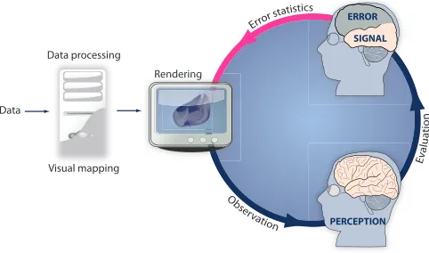
Previous approaches, even if they evaluated some perceptual error, did not use it for any improvement scheme, which is a part of our declarative concept. Our work presents amissing linkin the visual-ization pipeline shown in Figure 2 in red which opens a new field of possibilities.
2 PREVIOUSWORK
For two millenia, scientists have been trying to elucidate the mech-anisms in the human visual system (HVS) that are responsible for 3D shape perception. This topic remains an active area of multiple research disciplines such as psychology, neuroscience, computer sci-ence, mathematics, and physics. From the physics point of view, the sensory information is limited to patterns of light and is confined to their 2D projection on the retina. Using this sensory input, the HVS extracts information about the shape and the arrangement of objects with respect to their environment [34].
2.1 Perception of surfaces
The shape of an object is defined by the properties of its contour and its surface which does not change under similarity transformations. De-spite the fact that the 2D retinal projection of the object depends also on its orientation relative to the observer, the percept of the shape tends to remain constant. This phenomenon is calledshape constancy[28].
The HVS constructs a mental image of an object from a combina-tion of top-down cognicombina-tion and sensory input. At the lower sensory level, this includes the intensity variation of shading, texture gradi-ents, edges and vertices. At the higher cognitive level, it includes salient features such as occlusion contours (object-background separa-tion) [34]. Cole et al. showed that certain shape cues can be extracted solely from important lines, even though shape cues from shaded im-ages are more accurate [6]. However, shading alone cannot yield the depth structure of a scene correctly [7]. The depth cues from shad-ing are poor when compared to the retinal disparity (stereopsis) and kinetic cues [14].
Shading is specified by multiple parameters, i.e., the local surface reflectance properties, the angles between the surface normal and the direction of the light sources and the viewer. The judgment of shape is therefore a result of observers’ assumptions regarding several pa-rameters. The assumptions can vary between observers. Belhumeur et al. [2] introduced the termbas-relief ambiguity; when an unknown object with Lambertian reflectance is viewed orthographically, there
Data
Data processing
Rendering
PERCEPTION SIGNAL ERROR
Visual mapping
[image:3.567.288.529.53.195.2]Rendering
Fig. 2. The concept of iterative evaluation and design of a rendering technique. The original visualization pipeline contains no cycles and ends at the stage when the image is perceived by the user. The new concept contains a loop; The accuracy of perception is evaluated and the original rendering method is modified based on the measured error in perception.
is an implicit ambiguity in determining its 3D shape. For exam-ple, in a bumpy scene casting shadows, it is not possible to distin-guish whether the light direction is more slanted or if the bumps in the scene are deeper. The object’s visible surface f(x,y)is indistin-guishable from a generalized bas-relief transformation of the object
f(x,y) =λf(x,y) +µx+νy.
There is an evidence that thepictorial relief, i.e., the imaginary re-lief extracted from a 2D projection of a 3D scene, such as a rendering or a photograph, is systematically distorted relative to the actual struc-ture of the observed scene [7, 34]. The variations among observers’ judgments were revealed to be complex and thus could not be ac-counted for by a simple depth scaling transformation. However, subse-quent analyses showed that almost all of the variance could be roughly accounted for by an affine shearing transformation in depth [34].
Mamassian and Kersten investigated the perception of local surface orientation on a simple smooth object, under various illumination con-ditions [21]. They analyzed perceived local orientations for several points on the surface and quantified theslantandtiltof the local tan-gent plane. Byslant, we understand the angle between the surface normal and the view vector and, bytilt, the azimuth direction of the surface normal in the eye space [6]. This definition is illustrated in Figure 3. Mamassian and Kersten observed that slant was underesti-mated for slants larger than 20◦and overestimated under this value. This systematic error in slant perception results from the lack of visual reference and indicates that relative slant is a more robust cue [11]. Be-cause of the environmental cues, such as the presence of a frame [36], and the absence of binocular disparity [19], the brain receives informa-tion that the rendering is, in fact, flat. This informainforma-tion is in conflict with cues from shading and therefore, the mental image extracted from the rendering is flattened in a systematic fashion.
To resolve these ambiguities, the HVS tends to assume a cer-tain light direction [24]. Johnston and Passmore suggested that the slant discrimination declined with rotation of the light direction vec-tor towards the viewpoint [14]. Follow-up studies indicated that this direction is from above the viewer and 12◦ left from the vertical axis [33, 20]. O’Shea and colleagues studied the assumed slant of the light direction on purely diffuse surfaces with no shadows [26]. They demonstrated that the surface slants were most accurate when the light source was 20◦−30◦above the viewer.
N
V N
V
τ U
TILT
(a) (b)
P P
σ
[image:4.567.64.246.49.147.2]ρ A
Fig. 3. The slant angleθ is defined as the angle between the surface normalNat a pointPand the viewing vectorV.τdenotes the tangent plane atPandUthe up vector of the viewer’s coordinate-system. σis a plane such thatP∈σ andV⊥σ andρdenotes the plane defined by VandN. The tilt angleφis then defined as the angle in the left-handed system betweenUandA=ρ∩σin the halfplane (ρ,V) defined byN.
shape. The HVS treats specularities somewhat like textures, by using the systematic patterns of distortion across the image of a specular sur-face to recover 3D shape. Other studies also provide evidence about the influence of specular highlight on the perception of surfaces and demonstrate that the shininess of surfaces enhances the perception of curvature [25, 35].
Illustrators tended to exaggerate salient features such as curvature or important lines. Their methods have been mimicked by the graphics community. Exaggerated shading [29], geometry manipulation [15], light warping [37] and radiosity scaling [38] are good representatives. These techniques, however, were not derived from prior knowledge of a measured perceptual error. In contrast to prior work, we are pre-senting a novel concept where the visualization technique is based on a statistical model of the error in human perception. In particular, we target underestimation of surface slant of diffuse shaded surfaces. However, our concept can be applied to any self-chosen visualization technique that yields a measurable systematic error in perception.
2.2 Psychophysical experiments
The first experiments investigating human perception of 3D shapes were performed in the 19th century. The available information about these experiments is very poor, and therefore one should interpret their results with caution [34]. In the experiment of Mingolla and Todd [24], observers judged slants and tilts of numerous regions within shaded images of ellipsoid surfaces under varying illumination direction. The ellipses also had various shape, orientation and surface reflectance.
The works of Koenderink et al. [17] and Todd [34] describe the three most frequently employed experiments for probing perceived surfaces.
Relative depth probe task: Observers are exposed to a shaded surface. Two points on the surface are marked with dots of different colors. The observer is asked to choose which point he or she perceives closer in depth by pressing a dedicated key. Variations of this tasks were employed recently to assess visualization quality [18, 32].
Gauge-figure task: This task, designed by Koenderink et al. [16], allows one to determine the perceived orientation of a surface.
(a) (b)
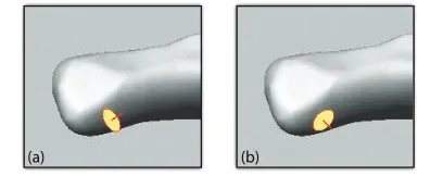
Fig. 4. Example of (a) a bad placement and (b) a good orientation of a gauge figure (red-yellow Tissot’s indicatrix) over a shaded surface.
It uses a Tissot’s indicatrix, i.e., an ellipse of distortion – a mathemati-cal tool that characterizes distortions from a map projection. When the indicatrix is aligned with a surface that is perpendicular to the viewing direction, it appears as a circle. When the surface is slanted from the viewing direction, it is seen as an ellipse. A gauge-figure consists of a Tissot’s indicatrix and a stick perpendicular to the plane defined by the indicatrix. On each trial, the observers’ task is to align the indicatrix with the perceived shaded surface. At the same time, the stick should be aligned with the surface normal at the point where it intersects the surface. In Figure 4, we illustrate an example of a bad and a good ori-entation of a gauge figure. This task has been employed for example by O’Shea et al. to measure the accuracy of surface perception under varying slant of the illumination direction [26]. ˇSolt´eszov´a et al. uti-lized this test to compare the surface perception for different styles of shadow rendering [32].
Cole et al. conducted a large-scale gauge-figure experiment, where they compared the accuracy of surface perception from automatic and man-made line-drawing representations of objects compared to their fully-shaded renderings [6]. Their experiment is the most relevant for our work. Their study was performed on 14 different images, both or-ganic and man made. On each object, they randomly selected 90, 180 or 210 positions. In all, they collected 275K solved gauge-figure trials accomplished by a total of 560 people and published this large dataset including user responses, datasets, scene settings and documentation.
Depth-profile adjustment mask: On each trial, observers are exposed to a shaded surface overlaid by aligned and equally spaced dots. In a second separate window, these dots are presented over a blank background and the observer is asked to adjust them so that they fit the perceived height profile defined by the dots in the first window.
Summary: Koenderink and colleagues compared these three tasks [17]. Coherent results can be achieved across observers and tasks. By far, the easiest and the most natural task to perform is the gauge-figure task. The judgment is instant, with no obvious reasoning; observers do not have to deduce their answers from their mental im-age. The pairwise depth-comparison task is also easy, but feels more boring and less natural. Observers have to abstract their answer from what they have perceived. It involves simple overt reasoning. The cross-section reproduction tasks feel not so much unnatural as indirect. With respect to reliability, the gauge-figure task is the most reliable.
3 PERCEPTUAL STATISTICS
In the original visualization pipeline, the data pass through the follow-ing stages until they reach the observer. After the acquisition stage, the data can be analyzed, filtered or processed in the data enhance-ment stage and later mapped to visual properties. Finally, the data are rendered and presented to the user. In some cases, the effect on per-ception is evaluated. Even though this is a step towards the perceptual aspect of visualization, the link from the evaluation back to the design of the rendering technique is practically non-existent.
In Figure 2, we show our new concept. We establish a new link that connects the results of an evaluation of a chosen rendering technique and the rendering technique itself. Starting from the rendering stage, the new pipeline now passes the following steps. The rendering is a distal stimulus which yields some sensory input which is interpreted by the HVS. This process is labelled perception. Evaluation refers to processing of the perceived information into the signal which corre-sponds to the ground truth and the error. Applying statistical methods to analyze the trends of the error allows us to model this error if it is systematic. This new knowledge is then sent to the rendering stage again. The rendering algorithm now becomes aware of the perceptual error it causes and can account for it.
[image:4.567.56.254.631.712.2]referenc e cur
[image:5.567.307.514.45.659.2]ve
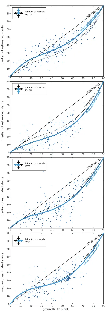
Fig. 5. Perceived surface slant as a function of the ground truth slant extracted from the dataset of Cole et al. [6]. Each dot represents the median of the entire set of trials at one sampling position. Theoverall estimation curveis a polynomial curve that is fitted to the data. The reference curvex=yindicates a perfectly accurate estimation.
3.1 Analysis of the perceived surface slant
The perception literature reports that the surface slant, as deduced from monoscopic renderings of 3D objects viewed on a screen, is system-atically distorted, however there is no model representing this phe-nomenon [26, 34]. The slant angle is understood as the angle between the surface normal and the viewing direction. We describe this effect with a mathematical model that was obtained through the statistical analysis of user responses. A model derived from statistical analy-sis of user evaluation has not been available before. It has been only attempted to model this effect as a parabolic function [26] or to use a simple shearing transformation in depth [34]. These approxima-tions are consistent with the general expectation of perception but not founded on a statistical analysis of results of a perceptual study.
We obtained our model by analyzing users’ responses collected as a publicly available dataset by Cole and co-workers as described in Section 2.1. The dataset contained results with fully-shaded and line drawing conditions. We analyzed only the responses for the fully-shaded condition. The line-drawing condition was completely ex-cluded. For each of the 1200 sampling positions, we obtained the ground truth normal including the slant and the tilt angles and a cor-responding set of normals estimated by the participants. In addition, for each sampling position, the authors of the dataset published the median of the corresponding set of estimates. They aimed to compare surface perception of 3D object representations on flat screens using monoscopic vision [6]. The overall dependency of the estimated sur-face slantθE and the ground truth θGslant is approximated with a
polynomial fitting curve of the 4thdegree and is shown in Figure 5. Theoverall estimation curveshows the trend of how humans tend to underestimate the surface slant. We originally computed different fit-ting curves with various specifications and obtained their goodness of fit (R2value) using the curve fitting tool of Matlab [22]. For various types of fit, we obtained the followingR2values: Fourier fit of 1st
de-gree –R2=0.773, Fourier fit of 8thdegree –R2=0.780, exponential fit –R2=0.774, cubic fit –R2=0.773, and for polynomial fits of 4th degree –R2=0.775, 5thdegree –R2=0.775 and 8thdegree –
R2=0.776. As a trade-off between the complexity of the fit and the goodness of fit, we chose the polynomial fit of 4thdegree.
However, the aggregated scatterplot in Figure 5 does not reveal a very interesting feature that is hidden in the dataset. We have sepa-rated the sampling positions into four groups according to the tiltφ
of the ground truth normal: normals pointing upwards or northφ∈
(315◦,45◦]; right or east φ∈(45◦,135◦]; downwards or southφ∈
(135◦,225◦]; and left or westφ∈(225◦,315◦]. We define tilt
(con-referenc e curve Azimuth of normals
NORTH
referenc e curve Azimuth of normals
SOUTH
referenc e curve Azimuth of normals
WEST
referenc e curve Azimuth of normals
EAST
[image:5.567.36.250.50.217.2]φ
φ
20°
40°
60° 80° 360° 0°
90°
180° 270°
θ*
θ 0°
80° 70° 60° 50° 40° 30° 20° 10°
90°
φ
φ
20° 40°
60° 80° 360° 0°
90°
180° 270°
θ
θ* 0°
80° 70° 60° 50° 40° 30° 20° 10°
90°
[image:6.567.37.542.49.258.2]g(θ,φ) = θ* g-1(θ*,φ) = θ
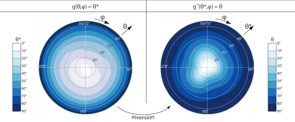
Fig. 7. Functionsg(θ,φ) =θ∗andg−1(θ∗,
φ) =θrendered as color-coded plots. Sincef=g−1, the right plot is also the look-up map which allows
to efficiently find the slant angleθof a normal which is perceived asθ∗.
sistently with the work of Cole et al.) as the azimuth angle on a com-pass where the wind directions areN=0◦,E=90◦, S=180◦and
W=270◦.
In Figure 6, we visualize the dependencies in each sector as scat-terplots and fitted curves. The distribution and thesector estimation curvesin the north and the south sector are very different. The slant of normals pointing north is underestimated less than average – the fitted curve is above theoverall estimation curve. For the normals pointing south the situation is opposite. These slants are more underestimated than average – the fitted curve is under theoverall estimation curve. The slant of normals pointing east and west are perceived very close to the average – theoverall estimation curve. This finding is consistent with the statement of Todd that the underestimation of slant cannot be compensated by simple scaling in depth but by a shearing transforma-tion in depth [34].
The crossing points of thesector estimation curvesand the refer-ence curvesindicate the thresholds between over and underestimation of slant. In our results, these thresholds correspond to approximately 15◦−25◦ of the ground truth slant with the exception of the south sector. Mamassian and Kersten [21] expect this threshold to be ap-proximately 20◦which is consistent with our finding of 15◦−25◦.
We also considered a similar factorization of samples according to the maximal curvature (low, middle, high) but we did not find any remarkable dependencies between the error and curvature.
3.2 The model of surface perception
In order to model the human perception of slant, we compute a 2D map f(θ∗,φ) =θwhich predicts that the slant angle of a surface nor-mal should beθ so that it is perceived asθ∗. We divide the samples into bins that represent eight sectors: north, south, east, west, north-west, north-east, south-north-west, south-east. To obtain this map, we pro-ceed as follows. For each sector, we calculate a polynomial fitting curve of the 4th degree. Four of these sector curves (north, south,
east, west) are plotted in Figure 6. These curves represent a function
gφ(θG) =θE which maps the ground truth slantθGin the sectorφ
to the estimated slantθE. For each curve, we set two boundary
con-ditions: the curve must intersect points(0,0)and(90,90)since it is expected that the estimation of these boundary values is correct. These boundary conditions also guarantee that all curves start and end with the same functional value ofθE and that the inverse functiong−φ1 is
defined on the whole interval of slant[0◦,90◦]. Forg−φ1, the following condition holds:g−φ1(θE) =θG. In other words,g−φ1predicts how the
slant angle of a surface normal should be so that it is perceived asθE
and therefore f(θ∗,φ) =g−φ1(θ∗).
So far, we have definedg−φ1for eight values of tiltφonly. In or-der to fill the missing values in the 2D map, we fit a smooth surface to the eightg−φ1aligned in polar coordinates according to their respective
φ. To fit the surface, we used the surface fitting tool of Matlab [22]. Color-coded height maps ofg(θ,φ)and f(θ∗,φ) =g−1(θ∗,φ)are shown in Figure 7. The height mapf, represented as a texture, allows for easy look-ups of the functional values offat runtime. This texture is publicly-available for download [31]. While this texture is the best possible representation of our model, sometimes a functional approx-imation of f(θ∗,φ)might be required. We found that ˜f, which is a
linear interpolationg−N=10◦and g−S=1180◦, yields very similar, however not identical, results. Withg−N1andg−S1as polynomials of 4thdegree
with coefficients (5.77e-6, -1.19e-3, 7.3e-3, 0.11, 0.0) and (4.21e-6, -6.73e-4, 1.88e-2, 1.69, 0.0) respectively, we define ˜fas follows:
˜
f(θ,φ) =|φ−180
◦
180◦ |g −1
N (θ) + (1− |
φ−180◦
180◦ |)g −1
S (θ) (1)
Ideally, the statistical model should be defined for each illumination algorithm individually because different algorithms might yield differ-ent response curves regarding the surface slant. We have obtained this model from renderings of objects from purely diffuse and opaque ma-terials. The mathematical model could be different for specular and shiny or semi-transparent surfaces.
4 THE STATISTICAL SHADING MODEL
I.A
VI.A
VI.B
I.B
II.A
II.B
III.B
III.A
V.A
V.B
VI.A
IV.A
IV.B
[image:7.567.29.535.48.408.2]III.A
III.B
III.B
Fig. 8. The Lambertian shading using original normals (A) versus statistical shading model (B) shown on various datasets: I – cervical and II – pulley [6], III – a CT scan of a mummy, IV and V are geometry representations of laser scans of a bunny and an angel, and VI – a stream surface.
A rendering of a given scene geometry (distal stimulus) using normal-based shading, evokes its corresponding mental image (proxi-mal stimulus) which can yield different perceived nor(proxi-mals as those of the original geometry. Our goal is to match the distal and the prox-imal stimulus, i.e., to specify a shading model where the normals of the mental image and the ground truth normals match. We achieve this by manipulating the normals that are input into our shading model using a perceptual model corresponding to the original shading algo-rithm. In Section 3.2, we described how to obtain such a model and its approximating function f(θ∗,φ) =θ. In our approach, we repre-sented this function as a 2D look-up table stored as a texture where each pixel with coordinates (θ∗,φ) stores the value of f(θ∗,φ) =θ. A color-coded representation of the look-up map and the coordinate system are shown in Figure 7.
A surface normaln= (x,y,z)has ground truth slantθGand tiltφG,
both given in projective space, but its slant is perceived asθ06=θG.
We shade the point with a modified normaln0= (x0,y0,z0)with slant
θ00=f(θG,φG)and with the same tiltφG. Notice thatθG=g(θ00,φG),
i.e.,θ00should be according to our theory perceived asθG. The
com-ponents of the modified normaln0are then defined as follows:
x0=√sin(θ00)
x2+y2x y
0=√sin(θ00)
x2+y2y z 0=cos(
θ00)
(2)
All illumination computation that follows is then executed with the new normalized surface normal||nn00||.
The concept of adjusting surface normals according to a given
per-ceptual model is applicable to any illumination computation scheme that is based on surface normals or gradients. To demonstrate the ef-fect of our approach, we applied our model to Lambertian shading and used purely diffuse-reflective materials. In all settings, the light source conforms to the assumed light direction [26]. Figure 1 shows a stream surface before (left-most) and after our modification (right-most). Fig-ure 8 contains more examples. A-images show the original shading with no modification of surface normals versus B-images showing our statistical shading. We included both datasets defined as volumes as well as geometry to show the general applicability of our technique. Objects I (cervical) and II (pulley) were also used by Cole et al. in their user experiment. Dataset III is a CT scan of a mummy visualized using gradient-based shading. Datasets IV and V were reconstructed from laser scans of a bunny and an angel. Dataset V is a geometry representation of a stream surface. All surfaces were shaded using Lambertian shading without (A) or with (B) modification of surface normals.
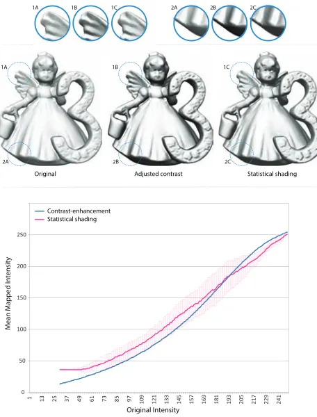
Adjusted contrast Statistical shading Original
1A 1B 1C 2A 2B 2C
1A
2A
1B
2B
1C
2C
Contrast-enhancement Statistical shading
0 50 100 150 200 250
1 13 25 37 49 61 73 85 97 109 121 133 145 157 169 181 193 205 217 229 241
M
ean M
apped I
nt
ensit
y
[image:8.567.314.526.48.165.2]Original Intensity
Fig. 9. Comparison of a contrast-enhanced image and a statistically-shaded image. We plotted the mean mapped intensities of a contrast-enhanced image and statistical shading. The error bars represent the standard deviationσof the mapped values.
5 VERIFICATION
Our hypothesis is thatthe modification of normals causes the estima-tion of surface slant to be closer to the ground truth. To obtain em-pirical support for our hypothesis, we studied perceptual judgments during the original shading condition (A) as opposed to our statisti-cal shading condition (B). We then formally analyzed the difference in performance between the two conditions.
5.1 The Experiment
In order to measure the effectiveness of our technique, we conducted a new gauge-figure experiment. Instead of just relying on the results of the experiment of Cole and co-workers [6], we again tested condition A (original shading). This assured an appropriate control baseline, as we used a different rendering framework. Cole et al. generated their images with YafaRay which is a free raytracing engine [40] and defined their source of illumination as an environment map. We em-ployed the commonly used Lambertian shading model and directional illumination.
We selected four distal stimuli from the experiment of Cole et al. – one organic dataset (cervical) and three man-made datasets (pulley, rockerarm, flange). Two of these stimuli are depicted in both shad-ing conditions, in Figure 8 – I. (cervical) and II. (pulley). The stimuli were viewed on a flat computer screen using the same camera settings and viewport size as Cole et al. For each stimulus, we selected re-spectively 41, 42, 39 and 38 sampling positions for placing the gauge-figure from Cole’s dataset. The positions were heuristically selected from the whole set in the following way. For each object, the ground truth slants were best-possibly distributed over the interval[0◦,90◦]
and the numbers of positions in each of four sectors (N,E,S,W) re-garding the ground truth tilt were also balanced. In total, we used 160×2 distinct test cases: 160 gauge-figure placing positions and two shading conditions for each position. Each participant solved 2/3 of
E
BE
AθG θE
[image:8.567.40.268.50.350.2]referenc e curve
Fig. 10. The error areas of a selected participant for the original shading condition A –EA(0◦,40◦)filled with pink and for our shading condition B
–EB(0◦,40◦)filled with blue.
400
300
200
100
0 Standard shading Statistical shading
Error ar
ea
Fig. 11. Interaction plot betweenEfor the two shading conditions: stan-dard (A) and ours (B) in each of four subintervals of the curve. The vertical bars denote the 0.95 confidence interval. We found a significant improvement in the interval[40◦,60◦]– blue, a non-significant worsening in[0◦,20◦]– red, and non-significant improvements in[20◦,40◦]and in
[40◦,60◦]– black.
all test cases so, in total, we collected at least 26 samples per test case and more than 8500 solved test cases overall. The collection of user responses is available for download [31].
Each of 40 participants attended two sessions. In each session he or she was tested on two pairs of stimuli with a 10 minute break between the pairs. The first pair of stimuli was presented in a different shad-ing condition than the second. Half of the participants started with shading condition A and the other half with the shading condition B. The order was selected randomly in the first session, but in the second session, the order of shading conditions was reversed. For example, a random participant might be first presented with the stimuli cervical and pulley, and the shading condition A, then he had a short break to avoid fatigue and he continued with stimuli flange and rockerarm and the shading condition B. When this participant came to the second ses-sion, he started with the rockerarm, the flange, and shading condition A, and continued with the cervical, the pulley, and the shading con-dition B. The number of samples per position was balanced between participants.
[image:8.567.310.524.221.357.2]0 500 1000 1500
0 500 1000 1500
-200 0 200 400 600 800
-200 0 200 400 600 800
-200 0 200 400 600 800
-200 0 200 400 600 800
-200 0 200 400 600 800
-200 0 200 400 600 800
-200 0 200 400 600 800
-200 0 200 400 600 800
0.00 0.05 0.10 0.15 0.20 0.00 0.05 0.10 0.15 0.20 0.00 0.05 0.10 0.15 0.00 0.05 0.10 0.15 0.00 0.05 0.10 0.15 0.00 0.05 0.10 0.15 0.00 0.05 0.10 0.15 0.00 0.05 0.10 0.15 0.00 0.05 0.10 0.15 0.00 0.05 0.10 0.15
Surface area error Surface area error Surface area error Surface area error Surface area error
Surface area error Surface area error Surface area error Surface area error Surface area error
D
ensit
y x 100
Shading c
ondition B
D
ensit
y x 100
Shading c
ondition A
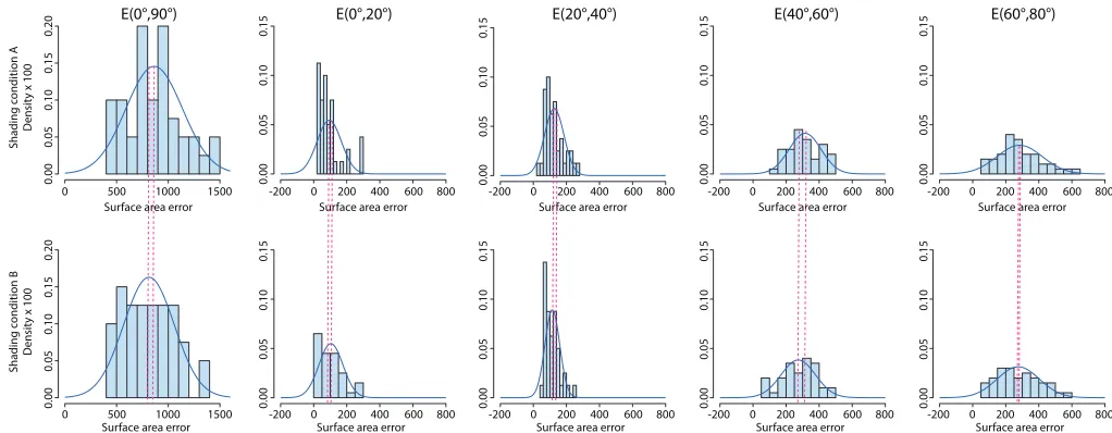
[image:9.567.23.534.47.246.2]E(0°,90°) E(0°,20°) E(20°,40°) E(40°,60°) E(60°,80°)
Fig. 12. Probability density of the surface area errorEwith histograms and approximative normal distribution curves for the entire interval[0◦,90◦]
and four subintervals[0◦,20◦],[20◦,40◦],[40◦,60◦], and[60◦,80◦]and for both shading conditions. In intervals[0◦,20◦]and[20◦,40◦], the normality of the distribution is violated which can be deduced from the histogram. The orange dotted lines indicate the difference between the mean values of the shading conditions within the same interval.
5.2 Accuracy measurement of participants
To determine the accuracy of each participant, we approximated his or her responses for each shading condition (A and B) by two polyno-mial fitted curves of the 4thdegreefA(θG) =θEand fB(θG) =θE.θG
andθE indicate the ground truth slant and the estimated slant
respec-tively. Each curve was computed from at least 106 samples. We define the error measureE(a,b)at an interval of slants [a,b] as the area of the surface enclosed by thereference curve R(θG) =θGand theuser
response curve U(θG) =θE:
E(a,b) =
Zb
a
||U(θG)−R(θG)||dθG (3)
In Figure 10, we show the estimation curves of a selected participant for each shading condition – red for A and blue for B. The figure also illustrates the meaning of the surface area in a selected interval of slant angles (a,b).
5.3 Analysis
To formally test whether the shading algorithm significantly improved participants’ accuracy, we compared the error areasEbetween the two shading conditions A and B for each of the 4 intervals of the curve, i.e.,E(0◦,20◦),E(20◦,40◦),E(40◦,60◦), andE(60◦,80◦). The divi-sion into subintervals was selected on a priori grounds. According to previous evidence [21] and also concluding from our own analysis, the underestimation of slant is zero at ca. 20◦ of ground-truth slant and highest for slants 40◦−60◦(see also Figures 5 and 6). Hence we predicted different effects in each subinterval.
We conducted a 4×2 repeated measures ANOVA with the curve interval (4 levels) as one factor and the shading condition (2 levels) as the other factor. Due to violations of sphericity according to Mauchly’s test, reported degrees of freedom and p-values are Greenhouse-Geisser corrected [10, 23]. The main effect of the curve interval was significant [F(1.5, 59.8) = 68.4, p<0.00001]. A trend towards a main effect of the shading condition failed to reach significance [F(1, 39) = 3.3, p = 0.08], although the area between ideal and obtained curves was numerically greater for the shading condition B (our new approach).
However, we obtained a significant interaction between the 2 fac-tors, indicating that the beneficial effect of our shading algorithm dif-fered for the different intervals of the curve [F(1.8, 70.9) = 4.2, p = 0.02] as shown in Figures 11 and 12. Difference contrasts showed that a significant benefit [F(1,39) = 12.4, p = 0.001, r = 0.49] of the algo-rithm was obtained for the interval[40◦,60◦]. Even though the error
bars indicating the 95%-confidence interval in Figure 11 do overlap, it does not imply that the effect is insignificant at 5% level [3]. For in-tervals[0◦,20◦],[20◦,40◦], and[60◦,80◦]respectively, p = 0.35, 0.10, and 0.56. The effect of shading algorithm at the first 2 intervals was re-checked with non-parametric Wilcoxon tests [39] due to violations of normality for those distributions in a Shapiro-Wilk test [30], but still failed to show significant differences (p = 0.23 and 0.09 respectively). Figure 10 illustrates that the difference in surface areas between the two user estimation curves in the intervals[0◦,20◦], [20◦,40◦], and
[60◦,80◦]is rather small compared to the interval[40◦,60◦]where the curves were expected to be further away from each other. Mean values and standard deviations of the error area distribution for each shading condition and for each interval of the curve are listed in Table 1.
In summary we found a highly significant effect of shading for an-gles in the interval[40◦,60◦]. Moreover, in this curve interval, our shading manipulation had an effect sizer=0.49 that would normally be regarded as impressively large within the psychological testing lit-erature [4, 5], accounting for 24% of data variance (r2=0.24). Ad-ditionally, the significance level of this effect was high enough to ex-clude arguments that the effect was a Type I statistical error caused by multiple sampling at different intervals.
5.4 Discussion
Based on the results obtained in our gauge-figure experiment, we cre-ated and applied a second model of correction as described in Sec-tion 3.2. Rendering results of this iterative process of evaluaSec-tion and re-design are illustrated in Figure 13.
We have shown that our modification of normals leads to more
ac-Table 1. ac-Table of mean valuesµand standard deviationsσfor the error area distribution within participants for each shading condition and each interval of the curve we analyzed.
EA(a,b) EB(a,b)
(a,b) µ σ µ σ
(0◦,90◦) 863.82 274.06 813.34 244.78
(0◦,20◦) 93.95 73.075 104.1862 72.59458
(20◦,40◦) 126.34 58.52 114.82 44.6
(40◦,60◦) 314.9 96.6 273.54 104.15
[image:9.567.306.518.661.732.2](a) (b) (c)
Fig. 13. Rendering results of a leopard gecko CT dataset of the iterative processevaluation and re-design: (a) the original Lambertian shading, (b) the result of a modification after the first user study, and (c) the result of a modification after the second user study.
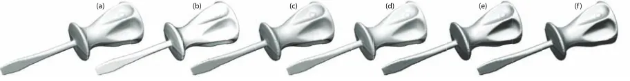
(a) (b) (c) (d) (e) (f)
Fig. 14. Comparison of (a) the Lambertian shading, (b) light warping, (c) exaggerated shading, (d) shearing along the z-axis and our approach using (e) the approximating functionf˜defined in Equation 1 and (f) the precise look-up texture to solve f(θ,φ,).
curate perception of normals slanted 40◦−60◦. Our technique is not photorealistic. One could ask whether this is the case for other tech-niques that mimic methods from illustration and visual art? Were il-lustrators aiming to improve perception? We do not have access to a perceptual evaluation of other existing illustrative techniques such as light warping [37], and exaggerated shading [29]. In Figure 14, we juxtapose these to simple shearing along the z-axis, and with statisti-cal shading in order to allow a subjective visual comparison. The two right-most visualization using the statistical shading model allow to compare the result of an approximative evaluation of f(θ,φ)as de-fined in Equation 1 using function ˜f and precise evaluation using the lookup map.
6 CONCLUSION
We described a new concept of the visualization pipeline which al-lows one to update the rendering algorithm with new knowledge about how the human visual system misperceives the shape of 2D object de-pictions. Specifically, we studied the perception of surface slant of Lambertian-shaded surfaces and found a systematic distortion. We captured this effect as a function which predicts how the surface slant should be presented so that it is perceived as the ground truth slant. The function allowed us to modify the surface normals or gradients in the Lambertian shading model in a manner that was shown, via empir-ical testing, to objectively improve slant perception. Even though the trend for improvement did not reach significance when pooled over all slant values, we found a significant improvement in the interval
(40◦,60◦)where the distortion of the slant perception is the highest.
6.1 Lessons learned
We found that the perception of normals pointing upwards in the eye space is clearly the most precise when compared to all other directions. Perception of normals pointing downwards is clearly the most inferior. Accuracy in the left and right directions is very similar. This character-istic of perception is illustrated in Figure 7 in the plot ofg(θ,φ). This shows that human ability to estimate surface slant is best on surfaces where normals point upwards and worst on surfaces where normals point downwards. We have not found a similar dependency of the es-timation error from higher order surface derivatives such as curvature.
6.2 Limitations and future work
We studied the distortion of human surface perception using stim-uli rendered with Lambertian shading of diffuse and opaque surfaces. Therefore, we cannot make a statement about this distortion if a dif-ferent rendering algorithm, e.g., shadowing or ambient occlusion, was
to be used, or if the objects were to be made of a different material, e.g., semi-transparent or shiny. Each rendering algorithm and material should be studied individually and provided with a perceptual distor-tion model which is an inspiradistor-tion for future research.
Since we have not evaluated the results after the second iteration, we are not able say whether the iterations really converge to a perfect solution. Shape cues are not formed solely from shading. Even though shape extraction from a shaded image is more accurate, Cole et al. showed that certain shape cues can be extracted from line drawings as well [6]. Our method does not modify important lines since we are not deforming the objects. Therefore, we suggest that our method can be combined with a perception-enhancing geometry deformation in order to achieve the best results.
We would like to raise awareness that since we modify shading, we also modify luminance in the final appearance of objects. Since the depth perception is affected by the luminance channel [19], it might be worthwhile investigating how our modified shading influences the depth cues. Even though our aim was to show the effect on shape perception of (local) surface slant, we would like to encourage future studies of depth perception as well.
The manipulation of shading can influence the appearance of ob-jects’ material. The reason is that variations in shape tend to dominate variations due to shading [38]. This effect is visible in Figure 13. As we apply iterative modification of normals, the surface appears more shiny. This observation opens a new interesting direction of research to attempt to characterize a model that adjusts the cues from shading and contours while preserving the appearance of the material.
We observed that techniques that mimic illustrators’ techniques are pursuing the same goal and, in our qualitative judgment, yield similar subjective effects. Speculatively, this suggests an intriguing hypoth-esis that illustrators used exaggeration of shading to better match the distal and the proximal stimulus.
ACKNOWLEDGMENTS
[image:10.567.63.519.193.252.2]REFERENCES
[1] Adobe. Adobe Photoshop CS4 - The “Curves...” tool. http://www. adobe.com/products/photoshopfamily.html, 2008. [2] P. Belhumeur, D. Kriegman, and A. Yuille. The bas-relief ambiguity.
International Journal of Computer Vision, 35(1):33–44, 1999.
[3] S. Belia, F. Fidler, J. William, and G. Cumming. Researchers misunder-stand confidence intervals and misunder-standard error bars. Psychological Meth-ods, 10(4):389–396, 2005.
[4] J. Cohen. Statistical power analysis for the behavioral sciences. Rout-ledge Academic Press, New York, 2ndedition, 1988.
[5] J. Cohen. A power primer. Psychological Bulletin, 112(1):155–159, 1992.
[6] F. Cole, K. Sanik, D. DeCarlo, A. Finkelstein, T. Funkhouser, S. Rusinkiewicz, and M. Singh. How well do line drawings depict shape?
ACM Transactions on Graphics, 28(3):28:1–28:9, 2009.
[7] E. De Haan, R. Erens, and A. Noest. Shape from shaded random surfaces.
Vision Research, 35(21):2985–3001, 1995.
[8] R. Fleming, A. Torralba, and E. Adelson. Specular reflections and the perception of shape.Journal of Vision, 4:798–820, 2004.
[9] A. Gallardo. Lambertian shading. In3D Lighting: History, Concepts and Techniques, page 117. Charles River Media, Inc., Massachusetts, 2001. [10] S. Geisser and S. W. Greenshouse. On methods in the analysis of profile
data.Psychometrika, 24:95–112, 1959.
[11] J. J. Gibson. The ecological approach to visual perception. Houghton Mifflin, Boston, 1979.
[12] B. Gooch, E. Reinhard, and A. Gooch. Human facial illustration: Cre-ation and psychophysical evaluCre-ation. ACM Transactions on Graphics, 23(1):17–44, 2004.
[13] D. H. House, A. S. Bair, and C. Ware. An approach to the perceptual opti-mization of complex visualizations. IEEE Transactions on Visualization and Computer Graphics, 12(4):509–521, 2006.
[14] A. Johnston and P. Passmore. Shape from shading. I: Surface curvature and orientation.Perception, 23:169–189, 1994.
[15] Y. Kim and A. Varshney. Persuading visual attention through geometry.
IEEE Transactions on Visualization and Computer Graphics, 14(4):772– 782, 2008.
[16] J. Koenderink, A. van Doorn, and A. Kappers. Surface perception in pictures.Perception and & Psychophysics, 52(5):487–496, 1992. [17] J. Koenderink, A. van Doorn, and A. Kappers. Ambiguity and themental
eyein pictorial relief.Perception, 30:431–448, 2001.
[18] F. Lindemann and T. Ropinski. About the influence of illumination mod-els on image comprehension in direct volume rendering. IEEE Transac-tions on Visualization and Computer Graphics, 17(12):1922–1931, 2011. [19] M. Livingstone. Vision and art – the biology of seeing. Abrams,
paper-back edition, 2008.
[20] P. Mamassian and R. Goutcher. Prior knowledge on the illumination po-sition.Cognition, 81:B1–9, 2001.
[21] P. Mamassian and D. Kersten. Illumination, shading and the perception of local orientation.Vision Research, 36(15):2351–2367, 1996. [22] MathWorks. Matlab: The language of technical computing. www.
mathworks.com, 2012.
[23] J. W. Mauchly. Significance test for sphericity of a normal n-variate dis-tribution.The Annals of Mathematical Statistics, 11(2):204 –209, 1940. [24] E. Mingolla and J. Todd. Perception of solid shape from shading.
Bio-logical Cybernetics, 53:137–151, 1986.
[25] J. F. Norman, J. Todd, H. Norman, A. M. Clayton, and T. R. McBride. Vi-sual discrimination of local surface structure: Slant, tilt, and curvedness.
Vision Research, 46:1057–1069, 2006.
[26] J. P. O’Shea, M. S. Banks, and M. Agrawala. The assumed light di-rection for perceiving shape from shading. InProceedings of the 5th symposium on Applied perception in graphics and visualization, pages 135–142, 2008.
[27] D. Pineo and C. Ware. Data visualization optimization via computational modeling of perception. IEEE Transactions on Visualization and Com-puter Graphics, 18(2):309 –320, 2012.
[28] Z. Pizlo and M. Salach-Golyska. 3-D shape perception. Perception and Psychophysics, 57(5):695–714, 1995.
[29] S. Rusinkiewicz, M. Burns, and D. DeCarlo. Exaggerated shading for depicting shape and detail.ACM Transactions on Graphics, 25(3):1199– 1205, 2006.
[30] S. S. Shapiro and M. B. Wilk. An analysis of variance test for normality (complete samples).Biometrika, 52(3–4):591–611, 1965.
[31] V. Solt´eszov´a. Perceptual-statistics web. www.ii. uib.no/vis/publications/publication/2012/
Solteszova12APerceptual, 2012.
[32] V. Solt´eszov´a, D. Patel, and I. Viola. Chromatic shadows for improved perception. InProceedings of the ACM SIGGRAPH/Eurographics Sym-posium on Non-Photorealistic Animation and Rendering, pages 105–116, 2011.
[33] J. Sun and P. Perona. Where is the sun?Nature Neuroscience, 1:183–184, 1998.
[34] J. Todd. The visual perception of 3D shape.Trends in Cognitive Science, 8(3):115–121, 2004.
[35] J. Todd and E. Mingolla. Perception of surface curvature and direction of illumination from patterns of shading.Journal of Experimental Psychol-ogy, 9(4):583–595, 1983.
[36] A. J. van Doorn and J. Koenderink. The influence of environmental cues on pictorial relief.Perception - ECVP Abstract Supplement, 29, 2000. [37] R. Vergne, R. Pacanowski, P. Barla, X. Granier, and C. Schlick. Light
warping for enhanced surface depiction.ACM Transactions on Graphics, 28(3):25:1–25:8, 2009.
[38] R. Vergne, R. Pacanowski, P. Barla, X. Granier, and C. Shlick. Improving shape depiction under arbitrary rendering.IEEE Transactions on Visual-ization and Computer Graphics, 17(8):1071–1081, 2011.
[39] F. Wilcoxon. Individual comparisons by ranking methods. Biometrics bulletin, 1(6):80–83, 1945.
![Fig. 1. The concept of iterative evaluation-analysis-redesign of a visualization technique is shown on a stream surface dataset.Analysis of the perceived surface slant while using a chosen shading model – the Lambertian shading model [9] on the left leads](https://thumb-us.123doks.com/thumbv2/123dok_us/1585107.111155/2.567.63.514.130.258/iterative-evaluation-analysis-visualization-technique-analysis-perceived-lambertian.webp)
![Fig. 8. The Lambertian shading using original normals (A) versus statistical shading model (B) shown on various datasets: I – cervical and II –pulley [6], III – a CT scan of a mummy, IV and V are geometry representations of laser scans of a bunny and an angel, and VI – a stream surface.](https://thumb-us.123doks.com/thumbv2/123dok_us/1585107.111155/7.567.29.535.48.408/lambertian-shading-original-statistical-datasets-cervical-geometry-representations.webp)