Efficient object tracking in WAAS data streams

Rochester Institute of Technology

RIT Scholar Works

Theses

Thesis/Dissertation Collections

2010

Efficient object tracking in WAAS data streams

Trevor Clarke

Follow this and additional works at:

http://scholarworks.rit.edu/theses

This Thesis is brought to you for free and open access by the Thesis/Dissertation Collections at RIT Scholar Works. It has been accepted for inclusion in Theses by an authorized administrator of RIT Scholar Works. For more information, please [email protected].

Recommended Citation

Efficient Object Tracking in WAAS Data Streams

by

Trevor R.H. Clarke

Thesis

Presented to the Faculty of the Graduate School of

Rochester Institute of Technology

in Partial Fulfillment

of the Requirements

for the Degree of

Master of Science

Committee:

Dr. Roxanne Canosa

Dr. Roger Gaborski

Reynold Bailey

Rochester Institute of Technology

Department of Computer Science

B. Thomas Golisano College of Computing and Information Science

Dedicated to Robert Clarke

for his never ending support

Acknowledgements

I would like to thank Dr. Roxanne Canosa for her excellent supervision and assistance. She

successfully steered me through the many obstacles and setbacks that come with pursuit of an

advanced degree.

I would also like the thank Dr. Bischof and the entire CS department support team. No research

endeavor can possibly succeed without a top notch group of support professionals.

This thesis would not be possible without high quality data. The Air Force Research Labs,

Persis-tent Surveillance Systems, the RIT College of Imaging Science, and Ball Aerospace and

Tech-nologies Corporation all provided data for use in this research.

Last but not least, thanks to my family and friends for motivating me to complete my work. I never

would have made it without the support of Jennifer, Bob, Susan, Raymond, and many more.

Abstract

Wide area airborne surveillance (WAAS) systems are a new class of remote sensing imagers

which have many military and civilian applications. These systems are characterized by long

loi-ter times (extended imaging time over fixed target areas) and large footprint target areas. These

characteristics complicate moving object detection and tracking due to the large image size and

high number of moving objects. This thesis evaluates existing object detection and tracking

al-gorithms with WAAS data and provides enhancements to the processing chain which decrease

processing time and increase tracking accuracy. Decreases in processing time are needed to

perform real-time or near real-time tracking either on the WAAS sensor platform or in ground

station processing centers. Increased tracking accuracy benefits real-time users and forensic

(off-line) users. The original contribution of this thesis increases tracking efficiency and

accu-racy by breaking a WAAS scene into hierarchical areas of interest (AOIs) and through the use of

Contents

Contents i

List of Figures ii

List of Tables iii

1 Overview 1

2 Thesis Objective 1

3 Background 2

3.1

RX Filter

. . . .

4

3.2

Nested Spatial Window Target Detector (NSWTD)

. . . .

4

3.3

Spectral Angle Mapper (SAM)

. . . .

5

3.4

Optical Flow Estimation

. . . .

5

3.5

RANSAC

. . . .

7

3.6

Hyperspectral Cueing

. . . .

7

3.7

Wang Tracking Algorithm

. . . .

7

3.8

Cohen Tracking Algorithm

. . . .

9

3.9

Camera motion compensation

. . . 11

4 Approach 11

4.1

WAAS Data Characteristics

. . . 11

4.2

Frame Segmentation

. . . 13

4.3

Motion Compensation

. . . 13

4.4

Object Detection

. . . 15

4.5

Object Tracking

. . . 15

4.6

Testing and Verification

. . . 16

4.7

Hyperspectral Cueing

. . . 17

5 Results and Discussion 18

5.1

Hyperspectral Anomaly Detection

. . . 18

5.2

Motion Compensation

. . . 19

5.3

Object Detection

. . . 20

5.4

Object Tracking

. . . 21

6 Conclusions 24

References 25

List of Figures

1

Tracking pipeline

. . . .

3

2

Sample frame from the CLIF dataset

. . . 12

3

An unbalanced quadtree decomposition has a higher depth in areas of

high object density.

. . . 14

4

Apparent motion due to parallax in frames 1 and 10 of CLIF-II dataset.

The motion is particularly noticeable with the building in the bottom

center of the images.

. . . 15

5

MISI K-RXD Results (in yellow)

. . . 18

6

CLIF-II Motion Correction

. . . 20

7

CLIF-II Object Detection

. . . 21

8

Tracks found in raw data (blue) and in data with camera motion removed

(orange)

. . . 22

9

Tracks found in data with camera motion removed (orange lines) and

ob-jects found using the automated method. The two colored blobs indicate

object locations in different frames.

. . . 23

10

Intersection detail with analyst tracks and automated object detection.

. 23

11

Spectral comparison of two car paint colors.

. . . 24

List of Tables

1

Properties of hyperspectral test data

. . . 17

2

Properties of datasets used for K-RXD timing

. . . 19

3

Execution times and throughput for K-RXD

. . . 19

4

Execution time and throughput for motion compensation

. . . 20

1 Overview

Wide area airborne surveillance (WAAS) systems are a new class of remote sensing imagers

which have many military and civilian applications. These systems are characterized by long

loi-ter times (extended imaging time over fixed target areas) and large footprint target areas. These

systems may be airborne or orbital and may contain sensors from any imaging modality

(syn-thetic aperture radar (SAR), hyperspectral (HSI), thermal (TIR), and electro-optical (EO) systems

have all been developed). The data streams generally have high spatial resolution and low

tem-poral resolution. A system from Persistent Surveillance Systems, for example, generates 96

megapixel EO frames at about 1 frame per second. There are two major difficulties created by

WAAS systems: a non-stationary camera makes tracking of moving objects difficult and tracking

the many objects in a scene is computationally expensive. The main contribution of this thesis

will be to adapt existing tracking algorithms to WAAS data streams. This is augmented by a target

nomination algorithm used to reduce the size of the tracking space.

WAAS systems often circle a fixed target area in order to increase loiter time. This generates

additional image motion which complicates object tracking. Existing tracking algorithms are

de-signed for use in fixed camera situations or traditional unmanned aerial vehicle (UAV) full motion

video (FMV). Much work has been done developing and adapting tracking algorithms for use

with standard UAV video. Wenshuai Yu[1] has developed a framework for moving target detec-tion and tracking for use with near real-time UAV video. Jiangjian Xiao[2] has shown two methods for tracking vehicles and people in UAV video. Isaac Cohen[3] has developed an algorithm which uses a directed acyclic graph of detected objects to register video and track objects even when

the object tracks are partially obscured.

These systems fail to address the second major difficulty with WAAS streams. Large target

foot-prints expose many targets (hundreds or more), many of which are partially obscured for portions

of the video sequence. Identifying and accurately tracking this many objects is a computationally

expensive operation. Human operators rarely need to track all of these objects simultaneously

and concentrate on an area of interest for near real-time exploitation. Target nomination using

supplemental HSI or other data will be explored as a way to shrink the tracking space. These

techniques will be demonstrated on data from the Air Force Research Labs Angel Fire project,

as well as data from aircraft mounted HSI sensors. The original contribution of this thesis is an

increase in tracking efficiency and accuracy by breaking a WAAS scene into hierarchical areas

of interest (AOIs) and through the use of hyperspectral cueing.

2 Thesis Objective

The objectives of this thesis are to determine the effectiveness of existing tracking algorithms

on WAAS data, increase the efficiency of existing algorithms on WAAS data, and increase the

There is a large body of prior research dealing with object tracking in airborne video data. Most

of this research deals with low spatial resolution, full frame rate EO video. A goal of this thesis

is to gauge the applicability of these techniques to WAAS data, which has high spatial resolution

and low frame rate. Existing algorithms will be modified to work on the lower frame rate WAAS

data and their effectiveness judged against human derived object tracks.

The lower spatial resolution video data typically used for object tracking constrains the number

of objects available for tracking. The high spatial resolution of WAAS data coupled with common

uses of this data, such as large event security monitoring, lead to a large number of objects which

need to be tracked. This can complicate tracking as there is a greater number of similar objects

following similar tracks. Determining which object belongs to which track and maintaining the

proper track can be difficult. This problem is also addressed by this thesis.

3 Background

Object detection and tracking are difficult with WAAS data. Large spatial resolution increases

the number of objects which need to be tracked and increases the computational requirements

needed for detection and tracking. The low frame rate also complicates tracking as object motion

predictions have greater variability from frame to frame.

Most object detection and tracking systems can be structured in a processing pipeline with a

number of common steps. Not all steps are present in all systems but this pipeline provides a

useful abstraction for comparison and evaluation of different techniques. The pipeline in Figure1

will be used for discussion.

Many WAAS systems use multiple cameras to capture the image data. These images need to

be mosaiced into a single frame. This is typically performed by the sensor’s internal processing

pipeline using a camera model specific to that particular imaging system. Generic mosaicing

algorithms exist but this thesis will assume that the sensor specific mosaicing algorithms are

sufficient and will concentrate on other portions of the tracking pipeline.

WAAS platforms are in motion relative to the ground so the apparent motion of objects in a video

sequence consists of the actual object’s motion combined with the motion of the WAAS platform.

Some algorithms require the platform to be stable so algorithms are needed to stabilize a video

stream relative to the ground. This stabilization may be accomplished by the platform’s mosaicing

algorithm but this stabilization is often coarse and may need refinement.

Object detection is a key step in the tracking pipeline. Detection algorithms may require multiple

video frames or a single frame for detection. There may be different methods of detection for

objects which are part of an existing track. A number of detection algorithms will be discussed in

[image:11.612.103.507.74.448.2]

Figure 1: Tracking pipeline

The primary decision point in the tracking pipeline determines if a detected object is in an

ex-isting object track or if it represents a new object. This decision may be implicit in the object

detection step if a separate algorithm is used to detect existing objects. Alternately, it may be an

explicit step in the pipeline. There are a couple of classes of tracking algorithms in general use.

Predictive tracking algorithms use existing information about a track and an object to estimate

where that object will reside in the next frame. This prediction is used to search for objects within

a threshold of the predicted location. The other class is matching algorithms. These algorithms

attempt to associate newly detected objects with existing tracks using a variety of metrics. If a

match is found, the track is extended; otherwise the object is considered new. Some algorithms

may implement a hybrid approach using data from both methods.

The object prediction step is used in predictive tracking algorithms to predict the next probable

location for an object. Matching algorithms use this stage to generate model parameters which

A number of algorithms will be presented and discussed below. Basic information on the

algo-rithm will be presented along with information on how the algoalgo-rithm has been used in existing

tracking applications. Some algorithms may encompass multiple stages in the tracking pipeline

or just a single stage.

3.1 RX Filter

A common anomaly detection algorithm, often used as a baseline anomaly detector for

com-parison with other algorithms, was developed by Reed and Yu [4]. This algorithm is commonly called the RX detector (RXD), RX filter, or simply RX. The classic expression of RXD is shown in

Equation1and is referred to as

K

−

RX D

.

δ

K−RX D

(

r

) = (

r

−

µ

)

T

K

−1

L×L

(

r

−

µ

)

(1)

The

K

refers to the sample covariance matrix,

r

is the

L

length vector of spectral intensities at

a particular spatial location and

µ

is the sample mean. A modification shown in Equation2uses the sample correlation matrix (R) and is sometimes used in optimized implementation since the sample mean is not needed. It is referred to as

R

−

RX D

to distinguish it from the covariance

version, K-RXD.

δ

R−RX D

(

r

) =

r

T

R

−1

L×L

r

(2)

Both forms of RXD are related to the Mahalanobis distance which measures the similarity

be-tween an unknown sample set and a known one. Further explanation of the properties and

application of RXD can be found in [5] and a number of other introductory texts on hyperspectral data exploitation.

3.2 Nested Spatial Window Target Detector (NSWTD)

NSWTD is an anomaly detection algorithm for hyperspectral data discussed in [6]. It can be used for object detection in a tracking pipeline. A group of three concentric spatial windows is used to

detect objects which are statistically distinct from their background. A spatially large window

con-tains a medium sized window and a small window. The two smaller windows represent potential

target sizes and the large window will be used to calculate the background statistics. NSWTD

uses a metric known as orthogonal projection divergence (OPD) shown in Equation3.

OP D

(

s

_i

,

s

_j

) =

Ç

s

_iT

P

_{s j}⊥

s

_iT

+

s

T_j

P

_{s i}⊥

s

T_j

)

P

_{s j}⊥

=

I

_L×L

−

s

_k

(

s

_kT

s

_k

)

−1

s

_kT

∀

k

=

i

,

j

(3)

Where

I

is an identity matrix,

s

T is the signal to noise ratio maximization operator from

The OPD equation must be calculated twice, once between the inner and middle windows as in

Equation4and once between the middle and outer windows as in Equation5.

δ

2W−N SW

1

(

r

) =

OP D

(

m

i n

(

r

)

,

m

d,1

(

r

))

(4)

δ

2W−N SW

2

(

r

) =

OP D

(

m

mi d

(

r

)

,

m

d,2

(

r

))

(5)

Where

m

_d,1 is the mean of the outer window minus the inner window and

m

_d,2is the mean of the outer window minus the middle window. Finally, the three window NSW is calculated by

Equation6.

δ

3W−N SW

(

r

) =

max

i=1,2

(

δ

_i2W−N SW

(

r

))

(6)

This gives a metric for each pixel which can be thresholded to determine if the pixel is

anoma-lous. According to [8], the NSWTD algorithm is faster than other, common anomaly detection algorithms such as RX while providing good detection results for targets of varying sizes.

3.3 Spectral Angle Mapper (SAM)

SAM is a common hyperspectral classification algorithm[9]. It can be used for object detection in a tracking pipeline or it may be used as an input to a matching-based object tracking algorithm.

Spectra are compared pair-wise by treating the spectral vectors as points in n-dimensional space,

normalizing to unit vectors, and calculating an angle between the two vectors. Since the vectors

are normalized, this method is invariant to illumination level. SAM is a way to quickly determine

similarity between two spectra and is a useful filter when the spectral angles are thresholded

against a fairly high target angle. Other spectral comparison algorithms provide more accurate

similarity results but SAM is extremely fast and is a good first cut for similarity filtering of pixels.

3.4 Optical Flow Estimation

Optical flow is the apparent motion of objects, surfaces, and edges between frames. This motion

is typically caused by motion of the camera and motion of individual objects in the scene. A

num-ber of methods are available for estimating optical flow but they generally fall into two categories.

Dense estimation techniques map all pixels in the first frame to corresponding pixels in the

sec-ond frame. Dense techniques are quite accurate and provide motion vectors for all the data in a

frame but are generally very computationally expensive. They are typically used on very small

scenes or subsets.

Sparse estimation techniques map a subset of pixels from one frame to another. This subset

may be an actual subset of pixels chosen by some external criteria or it may amalgamate pixels

into blocks and calculate the motion of the blocks. While less accurate, sparse techniques are

generally effective for calculating camera motion since a majority or pixels will have the same

The Lucas-Kanade (LK) [10] method was originally proposed as a dense estimation method but has since been adapted to become a sparse estimation method. LK can be used as a sparse

estimator since it only relies on spatially local information when estimating a pixel’s motion. The

motion of a subset of pixels can be calculated and these can be used as an estimate for the

motions of the other pixels.

The local information is derived from a small window around the pixel in question. This has a

serious drawback in that large motions which fall outside of this window can not be calculated. A

pyramidal version of LK can be used to overcome this deficiency. LK is first run on a low detail

version of the image, in essence a series of image blocks. This accounts for larger motions since

a window of a fixed size encompasses a larger percentage of the frame at a lower detail level.

This is repeated on one or more additional detail levels until the full detail frame is used.

LK make a few assumptions about the frames.

1. Brightness consistency - A pixel or object from one frame to another has fairly consistent

brightness levels.

2. Temporal persistence - A pixel or object makes only small movements. Small is not an

exact qualifier and relates to the overall size of the frame.

3. Spatial coherence - Neighboring pixels belong to the same surface, project to nearby

points on the image plane, and have similar motion.

These assumptions can be represented by equations7where

I

is the intensity of pixel

x

(

t

)

at frame

t

.

f

(

x,

t

)

≡

I

(

x

(

t

)

,

t

) =

I

(

x

(

t

+

d t

)

,

t

+

d t

)

∂

f

(

x

)

∂

t

=

0

∂

I

∂

x

|

t

(

∂

x

∂

t

)+

∂

I

∂

t

|

x(t)

=

0

v

=

−

I

t

I

_x

(7)

Starting with the brightness invariance and temporal persistence and applying the chain rule for

partial differentiation we end up with the second to last equation. We substitute

I

_x,

v

, and

I

_t for

each term to indicate the spatial brightness derivative, the velocity, and the temporal brightness

derivative. This yields the final form which is the basis for LK. The form indicated is the one

dimensional case but can be easily extended to two dimensions.

The change in space for a given time period is measured by finding strong corners in the edge

image of each frame. We search for corresponding corners in a local window and calculate an

so we use Newton’s method to refine the estimate using edge information in the spatial window.

A more in depth derivation of LK is available in [11] including a discussion of the strengths and weaknesses of the technique.

3.5 RANSAC

Random sample consensus (RANSAC) [12] is a method used to fit a model to observed data. RANSAC is an iterative method which is robust against outliers.

The algorithm works by randomly selecting a number of points from the observed data and fitting

a model to those points. Each point in the data which is not in this set is tested against the model

estimate. If the calculated error is less than a threshold it is added to a set of consensus points.

The algorithm is halted when the size of this consensus set exceeds a threshold or a maximum

number of iterations has occurred. The model with the largest consensus set is selected.

While robust, RANSAC has no upper bound on execution time. The maximum iteration count is

used to force an upper bound but exiting the algorithm this way results in a sub-optimal model. It

is possible to calculate the probability that RANSAC will generate a model with a maximum error

value and a maximum number of iterations. This information can be used to adjust these two

parameters in order to control the execution time or the margin of error.

3.6 Hyperspectral Cueing

Cueing as it relates to video tracking uses the video data or other, external data to mark candidate

objects or areas of interest. The supplemental data reduces the search space for the primary

tracking algorithm or supplements the primary tracking algorithm to increase the object detection

accuracy. Hyperspectral cueing uses external hyperspectral imagery to locate areas of interest

and to increase tracking accuracy. Anomaly detectors such as K-RXD locate areas of interest

based on spectral disimilarity. This areas of interest are intersected with the pixels flagged during

motion estimation. The other use of hyperspectral imagery is to supplement tracking of identified

objects. Objects in two frames of data are compared using a signature comparison algorithm

such as SAM. Comparing the spectral signatures of two objects provides additional information

when determining if these are the same object and thus constitute part of an object track.

3.7 Wang Tracking Algorithm

The tracking algorithm used by Wang, et al. [13] is a hybrid object tracking algorithm which uses matching-based and prediction-based techniques. Four values are examined to decide if an

object is a candidate for addition to a track: object trajectory, object size, grayscale distribution,

and object texture. Wang’s tracking algorithm requires a stabilized video stream. Stabilization is

estimate the bilinear projective model for the camera motion. [14][15] Object detection in Wang’s method utilizes a wavelet transform and the bilinear predictive camera model to remove camera

motion. The resultant differences between various levels of the wavelet pyramid identify objects.

Wang’s end goal is a motion prediction system which is used to compress video streams. Other

portions of the compression utilize the wavelet transform, so this is a process with zero additional

cost. The wavelet transform can be computationally expensive and will not be discussed in

further detail. It was used by Wang since the wavelet transformed needed to be calculated for

a non-tracking algorithm thus the data was already available for used for object detection. The

object tracking portion of Wang’s pipeline is of primary interest for this thesis.

Object position is defined in Equation8as the centroid of a detected object.

c

_x

= (

X

(i,j)∈O

p

_i,j

·

i

)

/

(

X

(i,j)∈O

p

_i,j

)

c

_y

= (

X

(i,j)∈O

p

_i,j

·

j

)

/

(

X

(i,j)∈O

p

_i,j

)

(8)

Where

O

is the set of coordinates of an object area and

p

_i,j is the value of the edge image at position

(

i

,

j

)

. Object motion over a few frames is assumed to be a straight line with constant

acceleration. Three frames are used to calculate speed

v

and acceleration

a

in Equation 9. These values predict a location for the current frame which is compared to the candidate object.

S

=

v t

+

1

2

at

2

(9)

With an adequate framerate, object size does not change significantly from frame to frame. A

dispersion value as calculated by Equation10is a metric for measuring object size. This equa-tion determines how far from the object centroid a nearly uniform gray level extends.

(

c

_x

,

c

_y

)

represents to object centroid from Equation8.

d i s p

= (

X

(i,j)∈O

q

(

i

−

c

_x

)

2

+(

j

−

c

_y

)

2

·

p

_i,j

)

/

(

X

(i,j)∈O

p

_i,j

)

(10)

Grayscale distribution (the width of the grayscale histogram) of an object is fairly constant for

objects of interest assuming the lighting conditions are constant from frame to frame. Grayscale

distribution is calculated as

(

g r

_m

,

g r

_h

,

g r

_l

)

the mean of groups of pixels in the entire range,

upper 10% of the range, and lower 10% of the range respectively.

The object texture measures grayscale variation across an object. Wang estimates texture by

of calculating the edge image is not discussed, but a reasonable assumption is that a common

edge detection method such as the Laplacian method or Sobel method can be used.

The four metrics discussed above are calculated for candidate objects and existing tracks (as

the object in the track for the previous frame). The difference between these sets of values is

thresholded and metrics outside the threshold are ignored. At least three of the four metrics

must be within the threshold for consideration. If no objects fit this criteria for a certain track, it

is terminated. If there is an unambiguous correspondence between a single object and a single

track, the track is extended. If multiple objects are candidates for a track, or multiple tracks

are candidates for an object, a weighted cost is calculated for each potential object and track

pairing using Equation11. The

w

variables represent the weights and the

f

and

t

superscripted variables represent the metrics for the current frame and the track. Wang was not clear how the

weights were determined, but it is implied that values were chosen which performed well with a

set of sample data.

d i f

=

w

_{t r}

(

|

c

_xf

−

c

_xt

|

+

|

c

_yf

−

c

_yt

|

)

+

w

_{d i s p}

(

|

d i s p

f

−

d i s p

t

|

)

+

w

_{g r}

(

|

g r

f l

−

g r

t l

|

+

|

g r

f m

−

g r

t

m

|

+

|

g r

f h

−

g r

t h

|

)

+

w

_{t x}

(

t x

f

−

t x

t

)

(11)

Wang’s algorithm is not expected to work well with WAAS data as stated due to the assumption

of a reasonably high frame rate in multiple steps in the algorithm.

3.8 Cohen Tracking Algorithm

Cohen and Medioni [3] present an alternate method for object detection and tracking as well as elimination of camera movement using optical flow. This system performs object detection and

matching-based object tracking.

Instead of directly modeling the 3D parameters of the camera motion, Cohen estimates the

in-duced optical flow of coincident frames. A small set of feature points

(

x

_i

,y

_i

)

in the image are

tracked from a reference image

I

₀ to a target image

I

₁. These two images are registered by computing the transformation

T

_I

1I0 which warps

I

0 to

I

1. The parameters are estimated using

an iterative minimization of the least square criterion as in Equation12.

E

=

X

i

(

I

₀

(

x

_i

,

y

_i

)

−

I

₁

(

T

(

x

_i

,

y

_i

)))

2

(12)

levels in an image pyramid. This transformation is incorporated into the optical flow calculation

according to Equation13.

∇

I

_i

∇

T

I

_i

w

=

−∇

I

_i

d I

i

d t

(13)

Where

w

= (

u

,v

)

T is the optical flow. This equation can be used to extrapolate the normal to

the optical flow in Equation14.

w

_⊥

=

−

(

I

i+1

(

T

i+1,j

)

−

I

i

(

T

i,j

))

||∇

T

_i,j

∇

I

_i

(

T

_{i j}

)

||

·

∇

T

_{i j}

∇

I

_i

(

T

_{i j}

)

||∇

T

_{i j}

∇

I

_i

(

T

_{i j}

)

||

(14)

w

_⊥ can be used to detect residual motion after compensation for optical flow. Large values of

w

_⊥ occur near regions of motion.

w

_⊥ is thresholded and a 4-connectivity scheme is used to aggregate points into regions of residual motion.

Cohen represents potential tracks using a graph. Nodes in the graph represent blobs detected

using the normal to the optical flow. Edges in the graph represent relationships between blobs

in coincident frames. Edges are created by measuring grayscale similarity between blobs in a

neighborhood. The size of the neighborhood is calculated based on the amplitude of the blob’s

motion. The eigenvalue of the potential transformation from a blob in

I

₀ to a blob in

I

₁ are attached to the associated edge. A set of attributes are also associated with each node. Cohen

associates the following attributes: frame number, centroid, principal directions, mean, variance,

velocity, parent ID and similarity, children IDs and similarities, and length.

Single objects may be detected as multiple blobs when using the optical flow normal. This

situa-tion can be detected in the graph when multiple blobs which are spatially close and have nearly

the same direction and velocity. When this occurs, the nodes on the graph are merged to a single

node and the edges updated accordingly. Detection accuracy of broken objects is increased by

maintaining a dynamic template for each object and matching it to potential broken objects. The

blob centroids and orientations are aligned over the last five detected frames and a median filter

is applied. Cohen calls this process amedian shape template. This filter can also detect objects

which stop and then resume motion. Each blob which has no connected components in

subse-quent frames will be propagated some number of frames into the future. The template for this

node is matched against nodes in these future frames and a positive match indicates an object

which has resumed motion.

Object trajectories can be extracted from the graph by finding an optimum path through the

c

_{i j}

=

C

i j

1

+

d

_{i j}2

(15)

An optimal graph path is then calculated from a node with no successors to a node with no parent

to determine an object trajectory.

Cohen’s algorithm is not expected to work well with WAAS data as stated. The need to build

a sizeable graph using many frames before tracks can be extrapolated lends itself to offline

data processing. Using low frame rate WAAS data may create a significant delay between data

collection and track determination, independent of processing resource requirements.

3.9 Camera motion compensation

The Columbus Large Image Format (CLIF) and CLIF-II data are used as a basis for motion

compensation and tracking. Data from a single camera in the six camera system is used. Since

a hierarchical subdivision of the image is used to target specific areas of the image to maximize

the throughput, using a spatial subset is equivalent to using the entire data set and setting focus

to the spatial subset. Scaling up processing to multiple machines would allow simultaneous

processing of these additional areas.

4 Approach

This thesis meets the objectives of increasing tracking efficiency and accuracy by breaking a

WAAS scene into hierarchical areas of interest (AOIs) and through the use of hyperspectral

cueing. The size of these AOIs and the number of AOIs which are actively processed will provide

a measure of control over the accuracy/efficiency ratio.

4.1 WAAS Data Characteristics

The primary datasets from the Air Force Research Labs are the Columbus Large Image Format

(CLIF[16] and CLIF-II[17]) datasets. Each are approximately 12000x5000 pixels spatially and were collected with a matrix of commercial digital cameras. The panchromatic frames are 8-bit

uncompressed. One dataset contains 50 frames and the other contains 56 frames. The data

were collected at approximately 2 fps.

The CLIF dataset has a number of camera registration issues resulting in overlapping areas

within the image. The data was acquired with a high off NADIR angle (side looking collection) and

contains light industrial and farmland areas. The registration makes accurate tracking difficult as

the unique location, the other data used is primarily urban, so this dataset is used for comparison

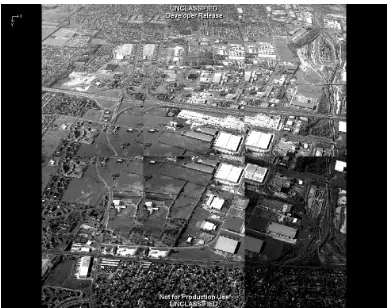
of execution speed but not for accuracy of object and track detection. A sample frame is show in

Figure2.

Figure 2: Sample frame from the CLIF dataset

Within the CLIF-II dataset, the areas captured by cameras 0 and 1 are used. A single camera is a

convenient region to use as it represents a reasonably sized subset of the data for the workstation

used for analysis, approximately 4000x2600 pixels.

The camera 0 area is a residential neighborhood with two multi-lane roads meeting at an

inter-section. A number of vehicles are in motion and there are a small number of pedestrians in

motion. Lighting is fairly constant and there are no large buildings showing significant parallax.

The camera 1 area contains the Ohio State University football stadium and the surrounding area.

A couple of tall buildings show parallax effects and there are some noticeable reflection, sun glint,

and shadow effects in and around the stadium. These effects add noise to the image which may

be mistaken for moving objects. A small number of vehicles are in motion but this portion of the

scene is mostly static.

Hyperspectral data from a number of sensors including NASA’s AVIRIS, RIT’s MISI, the US

[image:20.612.101.491.129.437.2]

scenes are shown in Table2.

No current collection system provides synchronized WAAS video and hyperspectral data required

for integrated performance analysis of the complete cueing system. Processing throughputs of

the individual compone

4.2 Frame Segmentation

An integral part of the optimizations of the various component algorithms is a hierarchical, spatial

breakdown of the WAAS data. A WAAS frame was segmented into smaller sub-images arranged

in a quadtree. The extent of the segmentation will vary based on the step in the tracking pipeline.

Breaking an image into smaller areas allows selective processing of a subset of the areas based

on expected processing requirements. When the average processing requirements of an AOI

exceed a threshold, the AOI can be further divided into four smaller AOIs and processing can be

limited to one or more of these.

This independent processing of a subset of the image allows for easy exploitation of parallel

com-puting capabilities. A number of AOIs can be processed independently on multiple computation

units. Processing of a greater number of concurrent AOIs could be accomplished by increasing

the number of available processing units. This aspect will not be fully explored by this thesis.

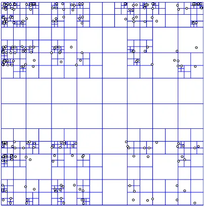
The frame segmentation is accomplished using a balanced quadtree whose leaf nodes contain

sub-frames of a reasonable (user defined) spatial dimension. When objects are being actively

tracked, further decomposition in areas of high object density can reduce processing load. Figure

3shows a sample quadtree decomposition of a scene.

4.3 Motion Compensation

Motion compensation of a sub-frame is accomplished by calculating the optical flow vectors

be-tween points in neighboring frames. A pyramidal implementation of the Lucas-Kanade (LK)

op-tical flow calculation method [10] is employed. The LK method is applied to various levels in an image detail pyramid of each sub-frame. This captures large motions using the LK method which

employs a small change detection window.

Sparse tracking is used to speed up calculations. Strong corners are located in an edge image

and these points are tracked between sub-frames. Once the optical flow vectors between these

points are calculated, RANSAC is used to approximate the motion of the sub-frame while ignoring

errors in the optical flow calculations.

The 3-D motion of the aircraft mapped to the 2-D image plane requires a perspective transform

[image:22.612.103.508.68.476.2]

Figure 3: An unbalanced quadtree decomposition has a higher depth in areas of high

object density.

An assumption is made that the altitude of the aircraft does not change significantly between

neighboring frames which allows a for a fairly accurate estimation of the sub-frame motion using

an affine transform. This assumption does not always hold particularly in urban environments

with many tall buildings. This fails to compensate for some of the parallax effect seen when

looking at these buildings. Parallax is the apparent motion of an object (usually rotation about

a point) due to differences in observation location. The CLIF-II dataset provides an example of

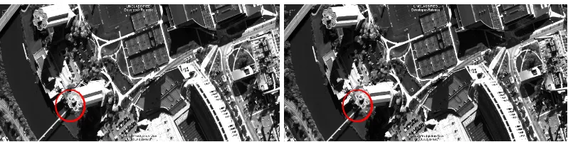
this as seen in Figure 4. The apparent motion of buildings may register as object tracks but these false positives are obvious to an analyst interpreting the data. Tracking extra objects may

slow down execution of the algorithm due to the additional data processing. Compensation for

parallax may be addressed in future work. Once the affine transform has been estimated, one of

[image:23.612.107.506.69.169.2]

Figure 4: Apparent motion due to parallax in frames 1 and 10 of CLIF-II dataset.

The motion is particularly noticeable with the building in the bottom center of the

images.

4.4 Object Detection

Two object detection methods are available depending on availability of hyperspectral data. When

hyperspectral data is available for a sub-frame, K-RXD is used to detect anomalous pixels in the

sub-frame. K-RXD was chosen instead of NSWTD as it is less sensitive to noise than NSWTD.

[18] provides a study of the accuracy and performance characteristics of a number of hyperspec-tral anomaly detection algorithms including RXD and NSWTD. NSWTD is potentially faster to

execute and has a higher correct detection rate for high signal to noise data and is worth further

exploration for future work.

When hyperspectral data is not available, frame differencing is used to remove the background.

The two sub-frames are thresholded to minimize brightness differences between the two frames.

Additional noise is removed by eroding the resulting threshold images. This removes single pixel

noise often called salt and pepper noise or speckle. The frames are subtracted from each other

to remove the background.

In either case, the resulting foreground or anomaly images are run through a morphological

opening to fill in small gaps internal to the object blobs. These blobs are labeled using connected

component labeling and each is treated as an object candidate.

4.5 Object Tracking

Object tracking was accomplished using a variation of Wang’s tracking algorithm.

Each object is added to a directed graph as a vertex. Objects from the base frame are connected

to the objects in the current frame and a number of properties are calculated on the vertices and

edges.

The vertices contain a dispersion value, an object blob centroid, and a hyperspectral spectra.

The edges contain the absolute difference of the dispersion values of the vertices and a velocity

track edge to the current edge. Both the absolute velocity magnitude difference is calculated and

the velocity vector angular difference. Finally, the spectral angle between the two objects is

calculated for each edge.

Edges with a velocity magnitude exceeding a threshold are removed. This is based on the

assumption that objects being tracked (usually vehicles and people) have an upper limit on their

speed. A cost is calculated on the remaining edges as a weighted sum of the edge properties. F

Tracking is performed within a quadtree AOI. As a track approaches the edge of an AOI, the

tracking algorithm is applied to the parent AOI in the quadtree. This larger area processing is

performed for a small number of frames until the location of the object in an AOI lower in the tree

can be determined. The object track information is passed to the new AOI for processing.

4.6 Testing and Verification

The following tests indicates the level of success for the thesis.

1. The efficiency of the hierarchical partitioning and hyperspectral cueing.

2. The accuracy of the tracking algorithm without hyperspectral object detection.

3. The accuracy of the hyperspectral object detection and track property.

Performance of the partitioning is determined by executing the tracking algorithm without any

par-titioning and comparing this to execution of the algorithm with various quadtree partition depths.

Throughput in terms of megapixels per second processed is the primary metric.

Comparison of the hyperspectral cueing performance is measured is megapixels per second

pro-cessed. This is compared to the collection rate of the hyperspectral sensor and to the processing

throughput of the optical flow differencing method.

Accuracy of the tracking algorithm is compared to human derived truth data. Two WAAS analysts

manually locate and mark objects and tracks in available data sets using techniques employed

by US Air Force intelligence services. These sets of truth data are compared and outliers

dis-carded. This technique may under-represent the number of objects and tracks in a data set but

should minimize the number of false positives. The accuracy in terms of number of correctly

iden-tified tracks, false positives, false negatives, and incomplete or interrupted tracks are the primary

[image:25.612.101.551.94.199.2]

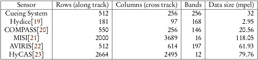
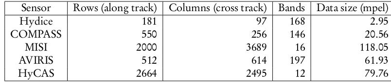
Table 1: Properties of hyperspectral test data

Sensor

Rows (along track)

Columns (cross track)

Bands

Data size (mpel)

Cueing System

512

256

256

32

Hydice

[

19

]

181

97

168

2.95

COMPASS

[

20

]

550

256

146

20.56

MISI

[

21

]

2000

3689

16

118.05

AVIRIS

[

22

]

512

614

197

61.93

HyCAS

[

23

]

2664

2495

12

79.76

4.7 Hyperspectral Cueing

No current collection system provides synchronized WAAS video and hyperspectral data required

for a complete hyperspectral cueing system as described in the background section. A

hypotheti-cal HSI collection system is used as the basis for hyperspectral cueing in the tracking system. The

properties of this system are consistent with current HSI imaging system technologies.

Perfor-mance of the system is characterized and conclusions are drawn about the utility of the system.

Future work may analyze integrated WAAS and hyperspectral data collections.

The system is a whiskbroom collector which contains a 256x256 pixel CMOS imaging array which

collects spectral information along one axis and spatial information along the other. Light enters

the system and is reflected off a rotating mirror, passes through a prism and is directed to the

detector array. The mirror slowly rotates which collects data across the second spatial dimension.

The speed of the mirror and extent of the rotation for which data is captured define the collection

rate and width of the collected swath. The size of the imaging array defines the height and each

swath and the number of spectral bands collected, 256 for each. Bands are in the visible and

near-IR spectral region; 400nm to 1000nm. A swath with a width of 512 pixels can be collected

in approximately 10 seconds including time to reset the mirror to the start position. The collection

platform can be moved such that a swath can be collected anywhere in the ground area covered

by the panchromatic WAAS imager. The maximum time to move the imager across the entire

WAAS field of view is less than or equal to 10 seconds. This means that the worst case collection

rate including repositioning of the imager is 20 seconds per swath. This yields a collection rate in

megapixels between 1.6

m pe l

/s

and 3.3

m pe l

/s

.

A number of existing hyperspectral sensor images have been used for experimental testing.

These sensors share some properties with the hypothetical system so they can be used to

ex-trapolate performance characteristics of the hypothetical system. All datasets contain data in

the visible and near-IR spectral regions providing complete or nearly complete overlap with the

5 Results and Discussion

5.1 Hyperspectral Anomaly Detection

The K-RXD implementation was tested on 5 hyperspectral data cubes and information on

per-formance was calculated. The resulting anomalous regions were reviews by 2 hyperspectral

data analysts to ensure the results are reasonable and correct. Validation is purely subjective

and the experience of the analysts is used to lend credibility to the opinions. The analysts

visu-ally inspected the spectra of a sample of flagged pixels to surrounding pixels. Inspection took

approximately 10 minutes per data set per analyst. In all cases, the analysts felt the indicated

anomalous regions are reasonable and correct. A visual comparison of the results with results

from a similar anomaly detection algorithm in the ENVI tool indicates nearly identical anomalous

pixels. The exact details of the ENVI detector are not known as that information is not made

avail-able in the documentation for the tool. ENVI is a frequently used tool for hyperspectral analysis

[image:26.612.106.508.319.462.2]

so it is reasonable to assume that it generates valid results.

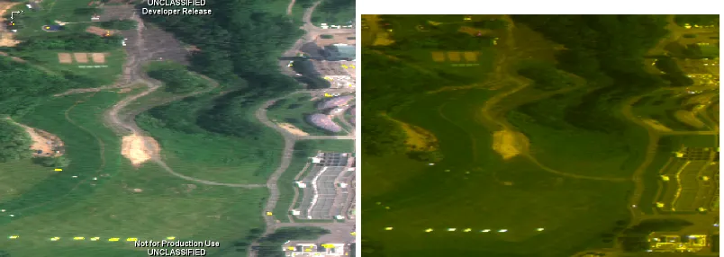
Figure 5: MISI K-RXD Results (in yellow)

The five data sets used have the following properties. Band counts do not include "bad bands"

which contain invalid data. This invalid data is usually due to atmospheric absorption spectral

regions which yield very low signal to noise values. In most cases data does not represent a

single swath either because the sensor is not a whiskbroom sensor or multiple whisks had already

been combined into a single image. All tests were run on a Windows XP 64-bit workstation with

4GB of RAM and an Intel Core2 E8500 dual-core CPU running at 3.17GHz.

Table3shows timing information for the K-RXD implementation. The values indicate the average of five executions of the algorithm for each data set. Absolute times are shown for the entire

algorithm execution minus the overhead introduced by unrelated processes such as graphical

display of the results and for the execution of the covariance matrix calculations. The data is also

presented as a throughput in terms of megapixels per second. The covariance matrix calculations

are performed by a separate plug-in which prevented certain optimizations such as calculation

[image:27.612.100.502.94.180.2]

Table 2: Properties of datasets used for K-RXD timing

Sensor

Rows (along track)

Columns (cross track)

Bands

Data size (mpel)

Hydice

181

97

168

2.95

COMPASS

550

256

146

20.56

MISI

2000

3689

16

118.05

AVIRIS

512

614

197

61.93

[image:27.612.102.508.220.294.2]

HyCAS

2664

2495

12

79.76

Table 3: Execution times and throughput for K-RXD

Sensor Execution Time (ms) Throughput (m pe l/s) Optimized Throughput (m pe l/s)

Hydice 3132 0.9417 1.310

COMPASS 20402 1.008 1.441

MISI 77315 1.527 2.737

AVIRIS 66685 0.9287 1.261

HyCAS 52016 1.533 2.762

the loop which calculate the sample mean has been removed and the throughput recalculated to

estimate the throughput of an implementation with this optimization.

This yields an average throughput across all the data set of 1.188

m pe l

/

s

and a standard

devi-ation of 0.3140. Applying the stated optimizdevi-ation, the average throughput is 1.902

m pe l

/s

and

a standard deviation of 0.7763. This is between 57% and 75% of the estimated collection rate of

the hypothetical hyperspectral sensor. It is clear that further optimization would be necessary to

maintain the hardware collection throughput. A faster processor or more highly optimized

imple-mentation seems within reach especially if the anomaly detection is performed on the collection

hardware using a highly optimized DSP implementation. The correlation matrix variant R-RXD

may also provide a more efficient implementation. Finally, the number of spectral bands in the

data strongly effects the calculation throughput. The number of bands increases the size of the

matrices and vectors in the RXD calculations which the spatial resolution effects the number of

times the RXD calculations are made. The higher order complexity of the RXD calculation (due

to three matrix multiplications) accounts for this effect. Minimizing the number of spectral bands

needed for adequate anomaly detection can also increase the throughput of the algorithm.

5.2 Motion Compensation

Table4shows timing information for the optical flow motion compensation implementation. The values indicate the average of five executions of the algorithm for each data set. Absolute times

are shown for the entire algorithm execution for a single frame. Times include overhead

intro-duced by informational display processes. The data is also presented as a throughput in terms

of megapixels per second.

[image:28.612.105.504.94.142.2]

Table 4: Execution time and throughput for motion compensation

Sensor Size (mpel) Execution Time (ms) Throughput (m pe l/s)

CLIF 61.28 6690.00 9.1645

CLIF-II camera 0 (vehicle traffic) 10.23 1769.64 5.8119

CLIF-II camera 1 (noise from sun glint) 10.23 2045.13 5.0079

deviation of 2.2047. These values suggest that processing has a noticeable per frame constant

overhead. Much of this can likely be attributed to informational data visualization which would

not be needed in a production implementation. Even though the current implementation does

not meet the expected 1fps data rate of the sensor, it is reasonable to a assume additional

optimizations and a faster CPU can achieve the desired processing rate at the single camera

[image:28.612.104.507.264.564.2]

resolution. This sensor has six cameras which can be processed on multiple compute cores.

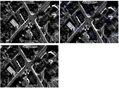
Figure 6: CLIF-II Motion Correction

from top left CLIF-II frame 0, frame 1 with optical flow vectors, frame 0 corrected

for sensor motion

5.3 Object Detection

Figure7shows two frames from the CLIF-II dataset. Optical flow camera motion correction has been applied to the frames. Objects detected from residual motion are shown and color coded

[image:29.612.107.506.94.154.2]

Table 5: Execution time and throughput for residual motion object detection

Sensor

Size (mpel)

Execution Time (ms)

Throughput (m pe l

/

s

)

CLIF-II full scene

61.40

3285.6

19.187

CLIF-II camera 0

10.23

476.68

21.476

CLIF-II camera 1

10.23

483.28

21.228

some cases only part of the object have been flagged. In another case, two cars passing each

other are flagged as the same object in frame 1.

Timing information for object detection for two sub-sets of the CLIF-II dataset are shown below.

Camera 0 contains an intersection with a number of moving vehicles. Camera 1 has fewer

moving vehicles and a significant amount of noise due to shadows and sun glint. The results are

averaged over 5 frame transitions. The standard deviation for the camera 0 data is 0.6146 and

for camera 1 is 0.4872. Full scene data is also included so that some information on scaling can

be inferred. The standard deviation for the full scene data is 1.629.

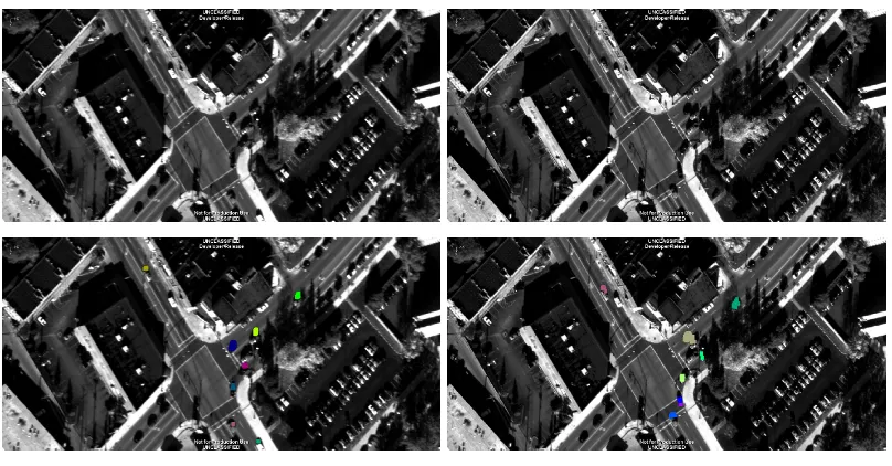
Figure 7: CLIF-II Object Detection

left to right from top CLIF-II frame 0, frame 1, frame 0 with detected object, frame

1 with detected objects

5.4 Object Tracking

A WAAS analyst was asked to locate moving objects and assign tracks over 5 frames of data. A

mission objective is always provided when WAAS analysis is performed. This allows the analyst

to limit evaluation to relevant data. The situation presented was a need to divert a VIP motorcade

through a residential neighborhood. The analyst was asked to provide a situational awareness

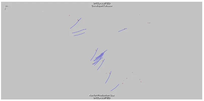
[image:29.612.104.508.319.530.2]

camera 0 scene. The blue tracks represent objects located in the raw data stream and the

green tracks represents objects located after camera motion was removed. The importance of

camera motion compensation can be seen by the number of additional tracks found after motion

compensation. Figure9shows a similar image comparing the analyst tracks to objects located using the automated method. Detail of the intersection is show in Figure10as this area of the data has a significant amount of activity. These images show that the analyst was able to locate

7 additional tracks, some of them indicating very little motion. These slower objects are people

which the algorithm has difficulty detecting. This is likely due to the various blurring operations

and morphological erosions which remove small detected object candidates. There are also a

number of tracks which the algorithm located but it required an additional frame of data. Looking

more closely at these locations indicates that the objects are obscured by shadows in all cases.

This results in dark areas a low signal to noise ratio which are likely removed during the threshold

[image:30.612.103.509.291.492.2]

portion of the object detection algorithm.

Figure 8: Tracks found in raw data (blue) and in data with camera motion removed

(orange)

Another problem can be seen in Figure10near the center of the image on the upper right road. Two cars are passing each other but the algorithm detects a single, multi-lobed object instead of

two distinct objects. Hyperspectral data for this scene is not available but if it were, the different

spectra of the two vehicles, due to different paint colors, would be used to distinguish the two

vehicles. Figure11compares the spectra of two vehicles with different paint colors.

Tracking objects which leave a sub-frame can be non-optimal in some circumstances as shown

in Figure12. An object moving outside of a sub-frame, represented by locations 1, 2, and 3, will reach the edge of sub-frame A at location 2. Tracking this object to location 3 requires processing

of a larger sub-frame. The next larger sub-frame is B but the edge of A is also the edge of B.

[image:31.612.102.508.71.269.2]

Figure 9: Tracks found in data with camera motion removed (orange lines) and

objects found using the automated method. The two colored blobs indicate object

locations in different frames.

Figure 10: Intersection detail with analyst tracks and automated object detection.

could be resolved by allowing arbitrary frames but this increases the number of possible

sub-frames. Another way to address this problem is to locate the adjacent sub-frame instead of using

[image:31.612.104.508.380.579.2]

[image:32.612.122.504.82.332.2]

Figure 11: Spectral comparison of two car paint colors.

6 Conclusions

The algorithms presented in this thesis are effective at compensating for camera motion in WAAS

data, locating objects of interest in hyperspectral and panchromatic WAAS data, and identifying

tracks between interconnected objects. The execution speed and throughput for these algorithms

is not sufficient to match the framerate of the WAAS data at full spatial resolution. Processing a

portion of the image using a quadtree decomposition on the frames maintains the framerate of

the data. The size of the processing area can be adjusted to match the processing capability of

the workstation.

The K-RXD hyperspectral anomaly detection algorithm is effective at locating spectrally distinct

areas in images with varying signal to noise. However, other anomaly detection algorithms may

be more efficient in terms of processing requirements. Further exploration of other anomaly

detection algorithms, especially NSWTD may decrease the processing requirements for

hyper-spectral cueing without serious effect on the quality of the results.

The lack of availability of coordinated hyperspectral and WAAS data collections prevents an

in-tegrated test of the proposed tracking system. While this thesis provides arguments that the

integrated system will prove efficient and effective in production situations, coordinated data

col-lections of both types of imagery are required to continue research on this topic. The increased

[image:33.612.104.508.68.475.2]

Figure 12: An object at locations 1, 2, and 3 in subsequent frames requires processing

of the entire image.

occur in the coming years. Testing the integrated system on operational data is of prime interest

for future research.

References

[1] Wenshuai Yu, Xuchu Yu, Penqiang Zhang, and Jun Zhou. A New Framework of Moving Target

Detection and Tracking for UAV Video Application.The International Archives of the Photogrammetry, Remote Sensing, and Spatial Information Sciences, 37:609–613, 2008.[cited at p. 1]

[3] I. Cohen and G. Medioni. Detecting and tracking moving objects for video surveillance. In Pro-ceedings of the IEEE Computer Society Conference on Computer Vision and Pattern Recognition, volume 2, pages 319–325. Citeseer, 1999.[cited at p. 1, 9]

[4] IS Reed and X. Yu. Adaptive multiple-band CFAR detection of an optical pattern withunknown

spec-tral distribution.IEEE Transactions on Acoustics, Speech and Signal Processing, 38(10):1760–1770, 1990.[cited at p. 4]

[5] C.I. Chang. Hyperspectral data exploitation: theory and applications. Wiley-Blackwell, 2007.

[cited at p. 4]

[6] W. Liu and C.I. Chang. A nested spatial window-based approach to target detection for

hyper-spectral imagery. In2004 IEEE International Geoscience and Remote Sensing Symposium, 2004. IGARSS’04. Proceedings, volume 1, 2004. [cited at p. 4]

[7] Joseph C. Harsanyi, Chein i Chang, and Senior Member. Hyperspectral image classification and

dimensionality reduction: an orthogonal subspace projection approach. IEEE Transactions on Geo-science and Remote Sensing, 32:779–785, 1994.[cited at p. 4]

[8] SR Soofbaf, H. Fahimnejad, M.J.V. Zoej, and B. Mojaradi. ANOMALY DETECTION ALGORITHMS

FOR HYPERSPECTRAL IMAGERY.[cited at p. 5]

[9] R.H. Yuhas, A.F.H. Goetz, and J.W. Boardman. Discrimination among semi-arid landscape

end-members using the spectral angle mapper (SAM) algorithm. InSummaries of the Third annual JPL airborne geoscience workshop, volume 1, pages 92–14. Pasadena, CA: JPL Publication, 1992.

[cited at p. 5]

[10] Bruce D. Lucas and Takeo Kanade. An iterative image registration technique with an application to

stereo vision. pages 674–679, 1981.[cited at p. 6, 13]

[11] Dr. Gary Rost Bradski and Adrian Kaehler.Learning opencv, 1st edition. O’Reilly Media, Inc., 2008.

[cited at p. 7]

[12] Martin A. Fischler and Robert C. Bolles. Random sample consensus: a paradigm for model fitting

with applications to image analysis and automated cartography. Commun. ACM, 24(6):381–395, 1981.[cited at p. 7]

[13] Y. Wang, J.F. Doherty, and R.E. Van Dyck. Moving object tracking in video. InProceedings of the 29th Applied Imagery Pattern Recognition Workshop, page 95. IEEE Computer Society, 2000.[cited at p. 7]

[14] S. Mann and R.W. Picard. Video orbits of the projective group: A simple approach to featureless

es-timation of parameters.IEEE Transactions on Image Processing, 6(9):1281–1295, 1997.[cited at p. 8]

[15] S. Lertrattanapanich and NK Bose. Latest results on high-resolution reconstruction from video

se-quences.IEIC Technical Report (Institute of Electronics, Information and Communication Engineers), 99(505):59–65, 1999.[cited at p. 8]

[16] Columbus large image format (clif) 2006 dataset. Website.

[17] Columbus large image format (clif) 2007 dataset. Website.

https://www.sdms.afrl.af.mil/datasets/clif2007.[cited at p. 11]

[18] Soofbaf, S.R., ValadanZoej, M.J, and Ashoori, H. Efficient Detection of Anomalies in Hyperspectral

Images.The International Archives of the Photogrammetry, Remote Sensing, and Spatial Information Sciences, 37:303–308, 2008.[cited at p. 15]

[19] R. Basedow, P. Silverglate, W. Rappoport, R. Rockwell, D. Rosenberg, K. Shu, R. Whittlesey, and

E. Zalewski. The HYDICE instrument design and its application to planetary instruments. In J. F.

Ap-pleby, editor,Advanced Technologies for Planetary Instruments, pages 1–+, 1993.[cited at p. 17]

[20] J. Zadnik, D. Guerin, R. Moss, A. Orbeta, R. Dixon, C. G. Simi, S. Dunbar, and A. Hill. Calibration

procedures and measurements for the COMPASS hyperspectral imager. In S. S. Shen & P. E. Lewis,

editor,Society of Photo-Optical Instrumentation Engineers (SPIE) Conference Series, volume 5425 ofSociety of Photo-Optical Instrumentation Engineers (SPIE) Conference Series, pages 182–188, August 2004.[cited at p. 17]

[21] J.R. Schott. Modular imaging spectrometer instrument (misi). InACSM/ASPRS Annual Convention and Exposition, February 1993.[cited at p. 17]

[22] G. Vane, R.O. Green, T.G. Chrien, H.T. Enmark, E.G. Hansen, and W.M. Porter. The airborne

visible/infrared imaging spectrometer (AVIRIS). Remote Sensing of Environment, 44(2-3):127–143, 1993.[cited at p. 17]

[23] NASIC. Hyperspectral collection and analysis system (hycas). Technical report, National Air

A Source Code Listing

The following pages contain source code listings for the test application. This source code builds

1 c:\Opticks\COAN\Tracking\Code\Tracking\Rx.cpp

1 _/*

2 * The information in this file is

3 * Copyright(c) 2010 Ball Aerospace & Technologies Corporation

4 * and is subject to the terms and conditions of the

5 * GNU Lesser General Public License Version 2.1

6 * The license text is available from

7 * http://www.gnu.org/licenses/lgpl.html

8 _*/ 9

10 _{#include "AoiElement.h"} 11 #include "AppVerify.h"

12 #include "BitMaskIterator.h"

13 #include "DataAccessorImpl.h"

14 #include "DataRequest.h"

15 #include "DesktopServices.h"

16 _{#include "ObjectResource.h"} 17 _{#include "PlugInArgList.h"}

18 _{#include "PlugInManagerServices.h"} 19 #include "PlugInRegistration.h"

20 #include "PlugInResource.h"

21 #include "ProgressTracker.h"

22 #include "RasterDataDescriptor.h"

23 #include "RasterElement.h"

24 _{#include "RasterUtilities.h"} 25 _{#include "SpatialDataView.h"} 26 _{#include "Rx.h"}

27 #include "ThresholdLayer.h"

28 #include <gsl/gsl_blas.h>

29 #include <gsl/gsl_matrix.h>

30

31 REGISTER_PLUGIN_BASIC(Tracking, Rx);

32

33 _Rx::Rx() 34 _{

35 _{setName("Rx");}

36 setDescriptorId("{55f85fb3-1a65-4686-9fdf-2c759383fbcb}");

37 setSubtype("Anomaly Detection");

38 setMenuLocation("[Tracking]/RX");

39 } 40 41 _Rx::~Rx() 42 _{ 43 _} 44

45 bool Rx::getInputSpecification(PlugInArgList*& pArgList)

46 {

47 VERIFY(pArgList = Service<PlugInManagerServices>()->getPlugInArgList());

48 VERIFY(pArgList->addArg<Progress>(ProgressArg(), NULL));

49 _{VERIFY(pArgList->addArg<RasterElement>(DataElementArg()));} 50 _{VERIFY(pArgList->addArg<SpatialDataView>(ViewArg()));} 51 _{VERIFY(pArgList->addArg<AoiElement>("AOI", NULL));} 52 return true;

53 }

54

55 bool Rx::getOutputSpecification(PlugInArgList*& pArgList)

56 {

57 VERIFY(pArgList = Service<PlugInManagerServices>()->getPlugInArgList());

58 _{VERIFY(pArgList->addArg<RasterElement>("Results"));} 59 _{return true;}

60 _} 61

62 bool Rx::execute(PlugInArgList *pInArgList, PlugInArgList *pOutArgList)

63 {

64 VERIFY(pInArgList);

2 c:\Opticks\COAN\Tracking\Code\Tracking\Rx.cpp

66

67 RasterElement* pElement = pInArgList->getPlugInArgValue<RasterElement> (DataElementArg());

68 SpatialDataView* pView = pInArgList->getPlugInArgValue<SpatialDataView>(ViewArg());

69 AoiElement* pAoi = pInArgList->getPlugInArgValue<AoiElement>("AOI");

70

71 if (pElement == NULL)

72 _{

73 _{progress.report("No element specified.", 0, ERRORS, true);} 74 _{return false;}

75 }

76 RasterElement* pCov = NULL;

77 { // scope

78 bool success = true;

79 ExecutableResource covar("Covariance", std::string(), progress.getCurrentProgress (), isBatch());

80 _{success &= covar->getInArgList().setPlugInArgValue(DataElementArg(), pElement);} 81 _{if (isBatch())}

82 {

83 success &= covar->getInArgList().setPlugInArgValue("AOI", pAoi);

84 }

85 success &= covar->execute();

86 pCov = static_cast<RasterElement*>(

87 _{Service<ModelServices>()->getElement("Inverse Covariance Matrix",}

TypeConverter::toString<RasterElement>(), pElement));

88 _{success &= pCov != NULL;} 89 if (!success)

90 {

91 progress.report("Unable to calculate covariance.", 0, ERRORS, true);

92 return false;

93 }

94 }

95 _{const RasterDataDescriptor* pDesc = static_cast<const RasterDataDescriptor*>}

(pElement->getDataDescriptor());

96 _{const BitMask* pBitmask = (pAoi == NULL) ? NULL : pAoi->getSelectedPoints();} 97 BitMaskIterator iter(pBitmask, pElement);

98 FactoryResource<DataRequest> pReq;

99 pReq->setInterleaveFormat(BIP);

100 pReq->setRows(pDesc->getActiveRow(iter.getBoundingBoxStartRow()), pDesc-> getActiveRow(iter.getBoundingBoxEndRow()));

101 _{pReq->setColumns(pDesc->getActiveC}