A methodology for the efficient computer representation of dynamic power systems : application to wind parks

Wind Energ. (2012) Published online in Wiley Online Library (wileyonlinelibrary.com). DOI: 10.1002/we.533

RESEARCH ARTICLE

A methodology for the efficient computer

representation of dynamic power systems:

Application to wind parks

Rafael Peña1_{, Aurelio Medina}1_{and Olimpo Anaya-Lara}2

1_{Facultad de Ingeniería Eléctrica, División de Estudios de Posgrado, Universidad Michoacana de San Nicolás de Hidalgo, Ciudad}

Universitaria, C.P. 58030, Mexico

2 _{Institute for Energy and Environment, University of Strathclyde , 204 George Street, Glasgow G1 1XW, UK}

ABSTRACT

This contribution presents a methodology to efficiently obtain the numerical and computer solution of dynamic power sys-tems with high penetration of wind turbines. Due to the excessive computational load required to solve theabcmodels that represent the behavior of the wind turbines, a parallel processing scheme is proposed to enhance the solution of the overall system. Case studies are presented which demonstrate the effectiveness and applications of the proposed methodology. Copyright © 2012 John Wiley & Sons, Ltd.

KEYWORDS

computer simulation; object-oriented programming; parallel programming; numerical differentiation; wind energy

Correspondence

Rafael Peña, Facultad de Ingeniería Eléctrica, División de Estudios de Posgrado, Universidad Michoacana de San Nicolás de Hidalgo, Ciudad Universitaria, C.P. 58030, Mexico.

E-mail: [email protected]

Received 22 January 2010; Revised 21 October 2010; Accepted 17 September 2011

1. INTRODUCTION

Power systems are under continuous evolution and demand for enhanced numerical techniques to effectively address the analysis and development of control strategies of modern power networks with increasingly large number of embedded generators. In recent years, the installation of wind turbines in power networks has increased considerably. Now the trend has moved from installations with a few wind turbines to the planning of large wind farms with several hundred megawatt of capacity.1This increase in wind power penetration makes the power network more dependent on, and vulnerable to, wind energy production. This situation leads to the necessity of developing mathematical models that represent adequately the electric and dynamic behavior of modern wind turbines.2In this way, simulation of the wind turbine interaction with the grid may thus provide valuable information and may even lower the overall grid operation and connection costs.3

Phase-domain models of the wind turbine have been used to model its dynamic behavior,4but these models represent an excessive computational load. For this problem to be addressed, two alternatives have been lately used. The first is the use of equivalent models that represent a group of turbines;5this alternative has the disadvantage that is not possible to study the particular behavior of each individual turbine. The second alternative is the use of models in the fictitious reference frame

dq0,6which in principle assumes perfectly balanced operating conditions in the machine. However, the models based on this assumption may not accurately describe the transient and steady-state unbalanced operation of the wind turbine. In this research, a parallel processing scheme is proposed to reduce the simulation time taken in the simulation of wind parks with a large number of wind turbines.

turbines using a specialized power systems software developed by the authors, namely ‘DGIS’, which stand for Distributed Generation Interactive Simulator.10 _{DGIS solves the automatically generated set of ODEs directly in the time domain in} a unified state-space representation. This representation based on the state-space formulation has the advantage that the trapezoidal rule of integration does not need to be applied to transform the equations that describe the behavior of the components of a power system, and also it avoids the need to define an impedance value, or a discretized Norton equivalent at the terminals of each network component.

The proposed methodology is illustrated using phase-domain models of the wind turbine to emphasize the benefits of the methodology as the number of generators increases. The rest of this paper is organized as follows: Section 2 explains the general structure and stages of the proposed methodology based on object-oriented programming (OOP) and parallel programming (PP); Section 3 presents a description about the software used and how the software takes advantage of the OOP to represent the power system elements as objects and then are connected using a numerical technique; Section 4 shows theabcmodel of a fixed-speed wind turbine used in this contribution; Section 5 presents a case study to show the benefits of the proposed methodology to wind energy applications; finally, Section 6 draws the main conclusions of this research work.

2. STRUCTURE OF THE METHODOLOGY

2.1. Overview

The simulation process of a power system using the proposed methodology is based on the following stages:

Graphical representation of the power system to be simulated. The power system is built by connecting functional blocks that represent each component of the system. These functional blocks may be assembled to build an electric power system of any complexity.

In these functional blocks, the information is stored about the equations and parameters that represent a particu-lar component of a power system. These functional blocks are then classified and stored in linked lists, one different linked list for each different component in the power system, e.g. they are classified into transformers, loads, machines, transmission lines, etc.

When all the equations and parameters that model the behavior of the system are known, a numerical solver is applied.

Since the numerical solvers used in this paper require evaluations of the ODEs in the time domain, this evaluation process is efficiently carried out using PP techniques.

After a simulation has been carried out, the user can select the results to be plotted as graphs in new windows, which can be saved as graphic elements or printed out; the numerical data can also be displayed in tables, which can be saved into text or Excel® files.

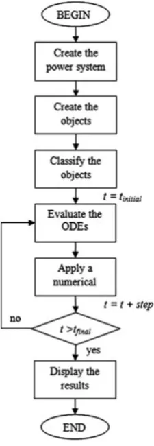
The flowchart in Figure 1 shows the process of simulating a power system using the proposed methodology. On each stage of the solution process, a different programming technique is applied (e.g. OOP, PP, etc), such that the solution process is carried out in an orderly and efficient way, as explained next.

2.2. Object-oriented programming techniques

The OOP technique is used in this paper to represent the power system elements as objects.11These objects contain the parameters, definitions, algorithms, algebraic and differential equations that model the dynamic behavior of the represented power system elements (e.g. electrical machines, transmission lines, loads, etc). The use of this computational technique also allows the creation of functional blocks, which are associated with a graphical element (icon); thus, these functional blocks can be used in a graphical user interface.

The power system can be built graphically by connecting these functional blocks; in computational terms, the elements of the power system are represented as objects, which are then classified and stored in linked lists.11Figure 2 shows the graphic representation of the elements of an electrical power system following the OOP technique.

Basic to the computer modeling of power system transients is the numerical integration of the ODEs involved. Consider the equation12

P

xDf .t ; x/ (1)

withx.t0/Dx0; there is a differentiable functionxDx.t /and an interval [t0,b], such thatx.t0/Dx0and

P

Figure 1. Simulation process of a power system using the proposed methodology.

Figure 2. Graphic representation of the objects in the object-oriented programming technique.

for allt 2[t0; b]. This means that the process of numerical integration is based on evaluations of the ODEs. An initial

conditions vectorx0 with the same size as the number of states that describe the dynamics of the power system under

analysis is required. The vectorx0is the solution to the non-linear system of equations defined byf .t0,x0/D0. Once the

2.3. Parallel programming techniques

Almost every modern operating system or programming environment provides support for concurrent programming. The most popular mechanism for this is some provision for allowing multiple lightweight ‘threads’ within a single address space that are used from within a single program. A thread is a straightforward concept: a single sequential flow of control. Having ‘multiple threads’ in a program means that at any instant the program has multiple points of execution, one in each of its threads.14

Although the application of PP using threads can be relatively simple, its application to solve a set of ODEs is not that straightforward. Since the numerical solvers are, by nature, ideal to be programmed in a sequential way, this means that one part of the algorithm is strongly connected to another part; in consequence, it is very difficult to split it up into several points of execution.15

For the maximum benefit from the use of PP techniques to be achieved,16,17_{in the proposed methodology, the evaluation} process of the ODEs is separated from the main numerical solver using threads, since this is an expensive task in terms of computational effort.

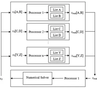
Figure 3 illustrates the application of threads to solve a set of ODEs; this is carried out in the following way: the linked lists (which contain the objects with their equations and definitions) are splitted up into several linked lists that are evaluated in separate threads, i.e. one linked list for each available thread. This division depends on the number of different linked lists available and the number of elements inside each linked list, e.g. if the system is only composed by wind turbines, then there will be only one linked list with several wind turbines inside; this means that it is necessary to split it up into several linked lists to be able to use threads.

When all the new linked lists have been formed, these are assigned to each available processor, then the evaluation pro-cess is carried out in parallel on the basis of an initial conditions vectorx0(which is splitted up too), and the evaluations

recollected in this process are stored in the vectorxeval; this vector is passed to the main numerical solver used to calculate the new state of the variables; this new state forms the new initial conditions vector for the next step. The numerical solver is applied in a sequential way (see Figure 3). This process is continued until the convergence condition is satisfied.

3. SOFTWARE DESCRIPTION

An interactive digital simulator named ‘DGIS’ developed by the authors has been used to conduct the studies. DGIS was developed in Visual C#, known as C sharp; it is a programming language designed for building a wide range of applications that run on the .NET Framework®. The main characteristics of C# are as follows: it is a simple general purpose program-ming language, type safe and object oriented, and it has the clarity, elegance and computational characteristics of C-style languages.

The software developed allows the modeling of generation and distribution system components and provides the neces-sary analysis tools to perform standard engineering calculations such as load flow and transient stability analysis, all in a user-friendly graphical interface.

The software has the same characteristics that are offered in similar simulation packages, i.e. it is based on a graphic platform, and the options of the software are accessed via windows, menus, icons and bars. Additional useful options are also included such as creation, saving and opening of existent projects, and printing and editing functions (e.g. redo, undo, delete, copy, cut and paste).

Distributed Generation Interactive Simulator software includes mathematical models for three-phase and single-phase elements. The included models are as follows:

Loads:18resistive, inductive and capacitive.

Electrical sources:18ideal and voltage sources modeled as a sinusoidal source behind an impedance.

Electrical machines:19,20_{synchronous and induction machines modeled in theabcanddq0reference frames.}

Transformers:9 three-phase models that include non-linear characteristics of the core, such as saturation and hysteresis.

Transmission lines:18pi-nominal and frequency-dependent models.

Wind turbines:6,21–23wind models, fixed-speed wind turbine with squirrel-cage induction generator, variable-speed turbine with double fed induction generator and variable-speed wind turbine with fully rated converter.

Photovoltaic panels:24series–parallel arrays, including the semiconductor characteristics.

Other models: ground, electrical nodes, meters and fault modules.

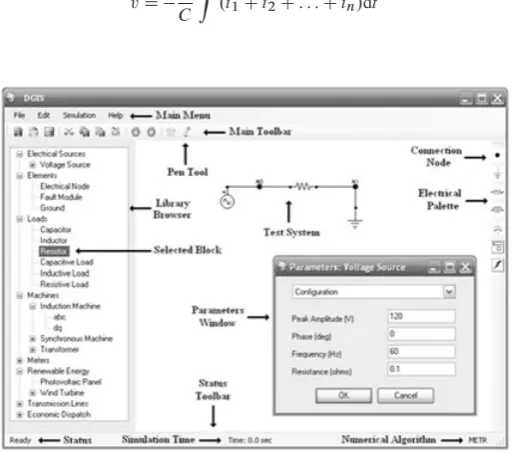
The icons for these models are shown in Figure 4. With these icons, an electric system can be built, and then a computational technique can be applied to analyze and study the electromechanical behavior of the system.

The methodology described in this work has been included as a kernel of the software, and it incorporates all the necessary functions and classes to be able to create, simulate and save the case studies.

3.1. Connection of functional blocks

The equations inside the functional blocks are modeled as voltage causal. This means that the input to any block is voltage and the output is current. Currents are then added at connection nodes, giving voltage as the output. The required voltage input to the connected blocks is given on the basis of the idea of the voltage equation of a fictitious small capacitor placed at the connection nodes.

Consider the voltage equation of a capacitor placed betweennfunctional blocks. The voltagevof this capacitor is given by equation 3.19

vD 1 C

Z

.i1Ci2C: : :Cin/dt (3)

whereC is the capacitance of the capacitor andi1,i2 andinare the currents flowing into the connection node. If the trapezoidal integration rule is used to relate voltage and current at the connection node, the following equations is obtained:

v.t /D˛

n

X

iD1

in.t /C n

X

iD1

in.tt /

!

Cv.tt / (4)

wheretis the simulation time step and

˛D t

2C (5)

4. FIXED-SPEED WIND TURBINE MODEL

Theabcmodel of a fixed-speed wind turbine used in this contribution is composed by a two-mass model of the wind turbine, equipped with an electromechanical model of a squirrel-cage induction generator.

4.1. Mechanical model

The torque equations describing the mechanical behavior of the wind turbine can be written based on a two-mass model as follows:21

d!wr dt D

TwrKs

Jwr

(6)

d!m dt D

KsTe

Jm

(7)

d

dt D.!wr!m/ (8)

whereTwr is the average aerodynamic torque (Nm),Teis the electromagnetic torque (Nm),Jwr andJmare the inertia constants of the wind turbine and the generator, respectively (kgm2/,is the angular displacement between the two ends of the shaft,!wr and!mare the frequency of the wind turbine and the generator rotor, respectively, andKsis the shaft stiffness (Nm rad1).

4.2. Induction generator model

The voltage equations in machine variables of a conventional squirrel-cage induction generator can be expressed as follows:20

vabcsDrsiabcsC dabcs

dt (9)

vabcrDrriabcrC dabcr

dt (10)

wherevare the voltages,rare the resistances,iare the currents andare the flux linkages. Thessubscript denotes vari-ables and parameters associated with the stator circuits,r subscript denotes variables and parameters associated with the rotor circuits, and theabcsubscript stands for variables and parameters in the phase-domain.

With the utilization of matrix notation, the machine currents can be written in terms of the winding inductances and flux linkages as follows:

abcs abcr D

Ls Lsr .Lsr/T Lr

iabcs

iabcr

(11)

whereLs,Lr,LmandLlare the stator, rotor, magnetizing and leakage inductances of the induction machine, respectively, and they are defined as follows:

LsD

2 6 4

LlsCLms 12Lms 12Lms 1₂Lms LlsCLms 12Lms 1₂Lms 12Lms LlsCLms

3 7

LrD

2 6 6 4

LlrCLmr 12Lmr 12Lmr 1₂Lmr LlrCLmr 12Lmr 1₂Lmr 12Lmr LlrCLmr

3 7 7

5 (13)

LsrDLsr

2 6 6 6 4

cosr cos

rC23

cosr23

cosr23

cosr cos

rC23

cos

rC23

cos

r23

cosr

3 7 7 7

5 (14)

For ap-pole induction generator, the electromagnetic torqueTedeveloped by the machine can be evaluated as follows:

TeDp

₂

3p3

Œa.ibic/Cb.icia/Cc.iaib/ (15)

5. CASE STUDIES

5.1. Connection nodes

The value selection of the constants in equation 5 for the calculation of voltages at the connection nodes is an important aspect to be considered. If the value of the capacitanceCor the simulation time steptis not small enough, then significant numerical noise may be introduced in the solution process.

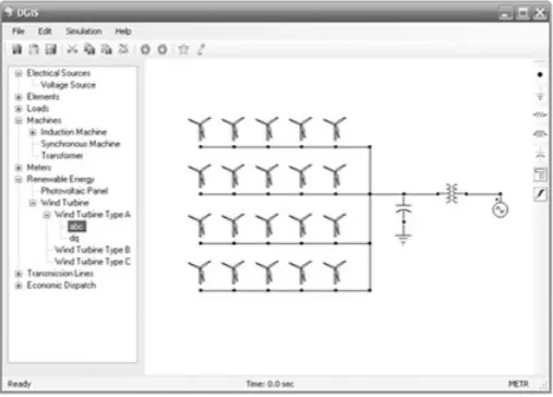
Figure 5 shows the configuration of the wind farm used in this paper and its implementation in DGIS. It consists of 20 fixed-speed wind turbines of 180 kW (which corresponds to the wind turbines installed in the Alsvik wind farm in the Island of Gotland).25This type of machine was selected because of the availability of the required data to model the fixed-speed wind turbine described in Section 4.25The wind farm is connected to an infinite bus through a transformer; a capacitor bank is included to compensate the reactive power requirements of the wind turbines.

For the effect of the capacitance selection and the simulation time step to be illustrated, a wind farm with 10 fixed-speed wind turbines was simulated. Table I shows a comparison of percentages of the maximum absolute error in the voltage calculation at the connection nodes, keeping˛at a constant value of0:05and using different values ofC andt. For the maximum absolute error in the voltage calculation at the connection nodes in comparison with the ideal case (i.e. without the need of this numerical technique) to be obtained, a model that represents the system under study was implemented.

From Table I, note that if small simulation time steps of the order of 10s are considered, then it is possible to define a small value ofC that will result in a minimized error in the calculation of the voltages at the connection nodes. For example, ifC D100 F and˛D 0:05, the maximum absolute error introduced in the system is around8:11104

%, and the time taken to complete the simulation will be acceptable (just a few seconds). Also, using this value ofC

(or smaller) prevents having to solve a stiff system.

Table I. Percentages of the error introduced in the calculation of voltage at the

connection nodes.

C (F) t (s) Absolute error (%)

10105 ₁₁₀5 _8:11104 10106 ₁₁₀6 _6:45105 10107 ₁₁₀7 _7:88106 10108 ₁₁₀8 _5:09107

On the other hand, if we assumetD10 ˜s, withCD100 ˜F, the error introduced in the system will be approximately

5:09107%, which improves the accuracy of the proposed technique, but at the expense of a longer simulation time, a couple of minutes or even more, depending on the period of time being simulated.

It should also be noted that the use of this technique adds three additional algebraic equations for each existent node in the system. However, with the utilization of this technique, the involved computational effort added for the wind farm simulation increases in only 0.2%; with modern processors, this computational effort increment may not be relevant.

5.2. Parallel numerical methods

Many of the new modern processors have support for the execution of multiple processes in parallel; hence, it is important when implementing new algorithms to take advantage of these facilities. In the proposed methodology, as the evaluation of the ODEs is carried out on a separate thread, it is possible to implement any numerical integration algorithm without the need to re-write all the necessary functions for the evaluation process, and the election of the numerical algorithm to solve the ODEs can be switched from one method to another in an easy way. The modified Euler, fourth-order Runge–Kutta and Runge–Kutta–Fehlberg methods were implemented to test the proposed methodology. The equations for these numerical methods are given in Appendix A.

Since the implementation of the PP has been designed for personal computers, the wind farms were simulated using an Intel® Core™ i7 CPU (2.67 GHz), 6.00 GB RAM PC. The initial conditions of the system were calculated using a conventional load flow method. The simulation time was 10 s with a step size of 1s for the three methods and a tolerance error of 1E05for the Runge–Kutta–Fehlberg method. For the case of the developed software, the proposed evaluation scheme to be executed in parallel was tested using 10, 20, 40, 80, 160, 320 and 640 wind turbines, respectively. The wind turbines configuration is illustrated in Figure 5.

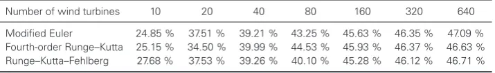
The percentages of reduction (PR) in the computational time required for the overall simulation using two threads com-pared with one thread for the three methods used is given in Table II. These percentages are calculated on the basis of the equation 16:

PRD

_T

STP TS

100% (16)

whereTSis the sequential time (i.e. using one thread) andTPis the parallel time, i.e. using several threads.

Note that the proposed parallel scheme achieves a better performance in larger systems with more components, e.g. the maximum reduction in the computational time was achieved with the use of the modified Euler method for the simulation of a wind park with 640 wind turbines; this reduction was 47.09%. On the other hand, the minimum percentage in the computational time reduction (24.85%) was achieved with the same method for the simulation of a wind park containing 10 wind turbines.

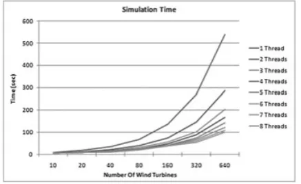
The same simulations were carried out using more than two threads; the maximum number of threads used was eight. Figure 6 shows the simulation time reduction achieved with the use from one thread and up to eight threads with the appli-cation of the modified Euler method. From this figure, it can be seen that for the wind park with 640 wind turbines, it took 539.64 s for the overall simulation using one thread, and using two threads, the computational time required for the overall simulation was reduced to 285.49 s; in percentage, this reduction is around 47.09%. This reduction is more evident

Table II. Percentages of the reduction of the time required to complete the simulation using two threads.

Number of wind turbines 10 20 40 80 160 320 640

Modified Euler 24.85 % 37.51 % 39.21 % 43.25 % 45.63 % 46.35 % 47.09 %

Fourth-order Runge–Kutta 25.15 % 34.50 % 39.99 % 44.53 % 45.93 % 46.37 % 46.63 %

Figure 6. Simulation time reduction using the modified Euler method.

if a comparison is performed for the overall simulation using eight threads. That is, using eight threads, it takes 99.24 s to complete the simulation; this represents a reduction of 81.60% in the overall simulation time.

ThePRof the time required to complete the simulation using eight threads for the three methods are shown in Table III. For this case, the results achieved using the three methods were quite similar, e.g. for the wind park with 10 wind turbines, the difference in percentage of the reduction in the simulation time with the three methods was around 2%; 3.5% for the case of 20 wind turbines and less than 1 % for the case of 40 wind turbines; the same happens for the case of 80, 320 and 640 wind turbines.

Comparing the results obtained with the three numerical methods, it can be observed that the proposed parallel scheme works well regardless of what numerical method is used; the results on the percentage of reduction of the simulation time are in every case very similar.

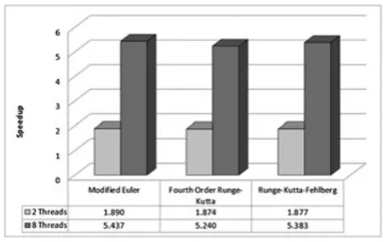
Another way to measure the speed gained by the use of a parallel technique is by means of the Speedup, defined as follows:14

SpeedupDTB TC

(17)

whereTBis the execution time of the base method andTCis the execution time of the method being compared. Generally, TBis measured using one thread, andTCis measured using any number of threads.

Figure 7 shows the speedup achieved by the modified Euler method for the wind park with 10 wind turbines, using from two to eight threads, respectively. It can be observed that for these eight case studies, the speedup is bigger than one, which means that the use of two or more threads significantly reduces the computational time required to complete a simulation. It can also be noticed that for this case, since there are a few components in the system, the higher speedup achieved is with the use of four threads; with the use of more than four threads, the speedup decreases; this means that the creation and synchronizations of threads take a significant time, in comparison with the time spent in the evaluation process of the ODEs.

Figure 8 shows the speedup achieved for the wind park with 20 wind turbines using from two to eight threads. For this case, the modified Euler numerical method was used. It can be observed that the speedup of the proposed parallel scheme has been increased, in comparison with the results obtained for the wind park with 10 turbines, e.g. using two threads, the speedup for a wind park of 10 wind turbines was 1.33, and now for the wind park with 20 wind turbines, the speedup is 1.60; the same can be observed if a comparison is made for the results obtained with the use of more threads. Besides, it is noticed that for this case, five threads are needed to obtain the highest possible speedup; this is a consequence of the increase in the number of system elements.

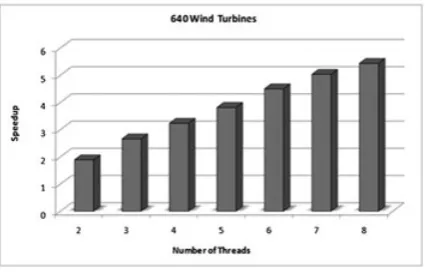
The speedup achieved for the simulation of a wind site of six 640 wind turbines is shown in Figure 9. It can be observed how the speedup is higher when the number of threads used in the simulation is increased, which means that the parallel implementation is working appropriately.

Table III. Percentages of the reduction of the time required to complete the simulation using eight threads.

Number of wind turbines 10 20 40 80 160 320 640

Modified Euler 39.00% 54.99% 70.57% 72.75% 74.27% 79.85% 81.60%

Fourth-order Runge–Kutta 40.99% 57.14% 70.58% 75.71% 79.06% 80.22% 80.89%

Figure 7. Speedup of the modified Euler method for the wind park with 10 wind turbines.

Figure 8. Speedup of the Modified Euler method for the wind park with 20 wind turbines.

Figure 9. Speedup of the modified Euler method for the wind park with 640 wind turbines.

Figure 10. Speedup of the methods using two and eight threads.

6. CONCLUSIONS

A methodology for the efficient numerical and computer representation of dynamic power systems with special reference to wind parks dynamics has been proposed. For the computational time required to complete a simulation to be reduced, object-oriented and PP techniques have been applied. The results obtained show the effectiveness of the proposed method for the analysis and study of wind parks with a large number of units, without the need for equivalent models to represent a group of turbines.

It was found that when the system under analysis has more components, a better speedup is achieved, e.g. up to 81.60 % of reduction in the time required to complete a simulation for a wind park with 640 wind turbines, using eight threads and the modified Euler method. One of the reasons for this behavior is that in simulations with a small number of elements, the computational time required by the creation and synchronization of threads becomes an expensive aspect of the numerical algorithm. It has also been shown that numerical methods used for the solution of the ODE’s can be easily adapted to the parallel scheme proposed without the need of any algorithm modification.

In addition, the DGIS software used in this research and some of its main characteristic have been presented. Also, a numerical technique has been applied within the software so that different components of the power system can be con-nected as functional blocks; thus, facilitating the representation of a power system of any complexity. Hence, this software and the parallel implementation proposed in this paper will assist in simulating the dynamic behavior of more complex wind parks.

APPENDIX A: NUMERICAL ALGORITHMS

Consider the problem

P

xDf .t ; x/ (18)

with initial conditionx.0/Dx0. Suppose thatxnis the value of the variable at timetn. The numerical differential solvers used in this contribution takexnandtnand calculate an approximation forxnC1at a short time later,tnCh, wheretis the simulation time step.

The numerical methods used are given by the following equations:

Modified Euler13

xnC1DxnCt

2

h

f .tn; xn/Cf .tnC1; x 0 nC1/

i

(19)

where

x_n0_C1DxnCtf .tn; xn/ (20)

Fourth-order Runge–Kutta13

xnC1DxnCt

where

k1Df .tn; xn/ (22)

k2Df

tnCt

2 ; xnC t

2 k1

(23)

k3Df

tnCt

2 ; xnC t

2 k2

(24)

k4Df .tnCt ; xnCtk3/ (25)

Runge–Kutta–Fehlberg26

In this method, the approximation to the ODE’s solution is made using a fourth-order Runge–Kutta method:

xnC1DxnCa1k1Ca2k3Ca3k4a4k5 (26)

And a better value for the solution is determined using a fifth-order Runge–Kutta method:

ynC1DxnCa5k1Ca6k3Ca7k4a8k5Ca9k6 (27)

The optimal step size can be determined by multiplying the scalarstimes the current step sizet. The scalarsis defined by equation 27.

sD

_et

2jynC1xnC1j

1=4

(28)

whereeis the specified error control tolerance and

k1Dtf .tn; xn/ (29)

k2Dtf .tnCb1t ; xnCb1k1/ (30)

k3Dtf .tnCb2t ; xnCb3k1Cb4k2/ (31)

k4Dtf .tnCb5t ; xnCb6k1b7k2Cb8k3/ (32)

k5Dtf .tnCt ; xnCb9k1b10k2Cb11k3b12k4/ (33)

k6Dtf .tnCb13t ; xnb14k1Cb15k2b16k3Cb17k4b18k5/ (34)

and the Runge–Kutta–Fehberg constants are as follows:

a1 = 25/216;a2 = 1408/2564;a3 = 2197/4104;a4= 1/4; a5 = 16/135;a6 = 6656/12,825;a7 = 28,561/56,430;

a8= 9/50;a9= 2/55;b1= 1/4;b2= 3/8;b3= 3/32;b4= 9/32;b5= 12/13;b6= 1932/2197;b7= 7200/2197;b8= 7296/2197;b9= 439/216;b10= 8;b11= 3680/513;b12= 845/4104;b13= 1/2;b14= 8/27;b15= 2;b16= 3544/2565;

b17= 1859/4104;b18= 11/40

ACKNOWLEDGEMENTS

REFERENCES

1. Slootweg JG, Kling WL. Modeling of large wind farms in power system simulations.IEEE Power Engineering Society Summer Meeting2002;1: 503–508. DOI: 10.1109/PESS.2002.1043286.

2. Chowdhury AA. Reliability models for large wind farms in generation system planning.IEEE Power Engineering Society General Meeting2005;2: 1926–1933. DOI: 10.1109/PES.2005.1489161.

3. Abderrazzaq MH, Aloquili O. Evaluating the impact of electrical grid connection on the wind turbine performance for Hofa wind farm scheme in Jordan.Elsevier Energy Conversion and Management2008;49: 3376–3380. DOI: 10.1016/j.enconman.2008.02.029.

4. Fajardo LAR, Iov F, Blaabjerg F, Hansen AD. Advanced induction machine model in phase coordinates for wind turbine application,IEMDC2007; 1189–1194, DOI: 10.1109/IEMDC.2007.383599.

5. Fernández LM, García CA, Saenz JR, Jurado F. Equivalent models of wind farms by using aggregated wind turbines and equivalent winds. Elsevier Energy Conversion and Management 2009; 50: 691–704. DOI: 10.1016/j.enconman.2008.10.005.

6. Erlich I, Kretschmann J, Fortmann J, Mueller-Engelhardt S, Wrede H. Modeling of wind turbines based on doubly-fed induction generators for power system stability studies.IEEE Transactions on Power Systems2007;22: 909–919. DOI: 10.1109/PES.2008.4596271.

7. Dommel HW.Electromagnetic Transients Program Reference Manual (EMTP Theory Book). EMTP User Group -BPA: USA, 1986.

8. Hoidalen HK. ATPDraw User’s Manual. Sintef, Version 3.5, 2002. [Online]. Available: ftp://ftp.ee.mtu.edu/pub/atp/ atpdraw/Manual/ (Accessed 8 January 2010).

9. Manitoba.EMTDC User’s Guide, Version 4.2. Manitoba HVDC Research Centre Inc: Canada, 2005.

10. Peña R, Medina A, Anaya-Lara O. An interactive visual enviroment based on advanced numerical and computer techniques for power systems applications,NAPS2009; 1–6, DOI: 10.1109/NAPS.2009.5484069.

11. Gross C.Foundations of Object-oriented Programming Using .NET 2.0 Patterns. Apress: New York, 2005. 12. Agarwal RP, O’Regan D.An Introduction to Ordinary Differential Equations. Springer: New York, 2008. 13. Mathews JH, Fink KD.Numerical Methods Using Matlab(4th edn). Prentice Hall: New Jersey, 2003.

14. Grama A, Karypis G, Kumar V, Gupta A.Introduction to Parallel Computing. Addison Wesley: London, 2003. 15. Korch M, Rauber T. Simulation-based Analysis of Parallel Runge–Kutta Solvers,PARA2004; 1105–1114.

16. Abbas A, Ahmad A. Object-oriented parallel programming,IEEE ISCON2002; 89–93, DOI: 10.1109/ISCON.2002. 1215945.

17. Shu J, Xue W, Zheng W. A parallel transient stability simulation for power systems.IEEE Transactions on Power Systems2005;20: 1709–1717. DOI: 10.1109/TPWRS.2005.857266.

18. Watson N, Arrillaga J.Power systems electromagnetic transients simulation. IEE Power and Energy Series 39: London, 2003.

19. Ong CM.Dynamic Simulation of Electric Machinery: Using Matlab/Simulink. Prentice Hall: New Jersey, 1998. 20. Krause PC, Wasynczuk O, Sudhoff SD.Analysis of Electric Machinery and Drive Systems. Wiley & Sons, Ltd.:

New York, 2002.

21. Ackermann T.Wind Power in Power Systems. Wiley & Sons, Ltd.: West Sussex, 2005.

22. Fernández LM, Saenz JR, Jurado F. Dynamic models of wind farms with fixed speed wind turbines. Elsevier Renewable Energy2005;31: 1203–1230. DOI: 10.1016/j.renene.2005.06.011.

23. Keyuan H, Shoudao H, Feng S, Baimin L, Luoqiang C. A control strategy for direct-drive permanent-magnet wind-power generator using back-to-back PWM converter,ICEMS2008; 2283–2288.

24. Minwon P, In-Keun Y. A novel real-time simulation technique of photovoltaic generation systems using RTDS.IEEE Transactions on Energy Conversion2004;19: 164–169. DOI: 10.1109/TEC.2003.821837.

25. Petru T, Thiringer T. Modelling of wind turbines for power system studies.IEEE Transactions on Energy Conversion

2002;17: 1132–1139. DOI: 10.1109/TPWRS.2002.805017.

26. Huang GM, Men K. Fast dynamic voltage stability margin estimation by integration with intelligent load adjustments.