A general perturbations method for spacecraft lifetime analysis

A GENERAL PERTURBATIONS METHOD FOR SPACECRAFT

LIFETIME ANALYSIS

Emma Kerr,

Malcolm Macdonald

An analytical atmospheric density model, including solar activity effects, is ap-plied to an analytical spacecraft trajectory model for use in orbit decay analysis. Previously presented theory is developed into an engineering solution for practi-cal use, whilst also providing the first step towards validation. The model is found to have an average error of 3.46% with standard deviation 3.25% when compared with historical data. The method is compared to other analytical solu-tions and AGI’s Systems Toolkit software, STK. STK provided the second best results, with an average error of 11.39% and standard deviation 10.69%. The developed method allows users to perform rapid Monte-Carlo analysis of the problem, such as varying launch date, initial orbit, spacecraft characteristics, and so forth, in fractions of a second. This method could be used in many practical applications such as in initial mission design to analyze the effects of changes in parameters such as mass or drag coefficient on the lifetime of the mission. The method could also be used to ensure regulatory compliance with the 25-year end-of-life removal period set out by debris guidelines.

INTRODUCTION

Spacecraft lifetime analysis is typically performed numerically, due to its perceived accuracy, an approach that can be time-consuming and computationally expensive. A general perturbations method is therefore preferable, especially in cases such as initial mission analysis where many different scenarios may be studied to produce the optimum mission specifications or regulatory compliance. The use of general perturbation methods to predict the lifetimes of spacecraft in low eccentricity orbits has received significant attention in the literature however, to date reliable pre-dictions remain wanting due to the time dependent nature of the problem.

The calculation of spacecraft lifetimes is challenging due to unknowns in the calculation pro-duced by uncertainties in factors such as the position and attitude of the spacecraft, or the accura-cy of the atmospheric density data applied. These uncertainties can be minimized by extensive study and testing, however they can never be completely removed leaving an inherent error in any lifetime calculation as they are dependent on predicting the future behavior of the solar cycle and hence the atmosphere, which is inherently unpredictable.

*

PhD Candidate, Advanced Space Concepts Laboratory, Department of Mechanical and Aerospace Engineering, Uni-versity of Strathclyde, James Weir Building, 75 Montrose Street, Glasgow, G1 1XJ.

†

Associate Director, Advanced Space Concepts Laboratory, Department of Mechanical and Aerospace Engineering, University of Strathclyde, James Weir Building, 75 Montrose Street, Glasgow, G1 1XJ.

Atmospheric friction (commonly referred to as atmospheric drag) is the main contributor to spacecraft decay, therefore accurately modelling it is vital when producing a lifetime prediction. However, to do so the stochastic nature of the solar flux affecting the atmospheric density must be considered. When solar flux is introduced to the atmospheric density calculation, which in turn is applied to the atmospheric drag calculation, the solution becomes inherently time-dependent due to the variations within the solar cycle.

The most commonly cited general perturbations method of predicting the lifetime of low-eccentricity spacecraft is the method presented by Cook, King-Hele & Walker and later expanded by King-Hele, herein called the King-Hele method.1,2 The method is based on power series ex-pansions of the eccentricity, semi-major axis and eccentric anomaly. It is also worth mentioning the technical report by King-Hele & Walker that dealt with a lifetime prediction theory using the current decay rate, though the theory is subject to more uncertainty and is therefore less suitable.3 Griffin & French present a general perturbations method for spacecraft in circular orbits, which was developed from the King-Hele method but makes no significant advances on it.4 None of these methods incorporate the effect of solar flux on the atmosphere.

Predicting future variations in the solar cycle, as is required for accurate orbit decay modeling, has received significant attention. For example, Schatten has published extensively in conjunction with various other authors on the solar cycle and solar activity.6,7,8,9 However, this work was not applied to the prediction of spacecraft lifetimes until Naasz, Berry & Schatten showed that the level of solar activity directly affects the lifetime of a spacecraft; high levels produce shorter life-times while low levels produce longer lifelife-times.10

Vallado & Finkleman put the discussion of solar cycle variation in terms of the effect on spacecraft lifetime prediction, again finding that there was a direct relationship between the level of solar activity and spacecraft decay rates.12 More specifically they found that solar flux was the largest contributor to variations in atmospheric density. They also discuss the solar radio micro-wave flux F10.7 index, which is commonly used as an indicator of the solar activity level, and its

use in empirical models of atmospheric density, finding that it is the most suitable proxy for solar activity.12 Further to studying the solar cycle in general terms many studies have focused specifi-cally on the shape of the solar cycle, and its apparent deviation from a typical periodic sinusoidal form.13,14,15 Capturing this deviation is critical to gaining an accurate model of the solar flux.

A basic theory for lifetime prediction has previously been developed by the authors, which in-corporates the effect of solar activity directly into the atmospheric density model. This paper de-velops the theory into an engineering solution for practical use, and provides the first step towards validating and testing the method.

THE MODIFIED KING-HELE METHOD

im-year cycle it should be noted that individual cycles may be as short as 9 im-years or as long as 14 years.15 A direct relationship between sunspot number and solar flux levels, to link solar flux ac-tivity levels to atmospheric density using the density index, was then introduced using the shape equation developed by Hathaway et al. for use with sunspot numbers.15,16

Finally, from Lagrange’s planetary equations, equations were derived that provide a prediction of a spacecraft’s expected lifetime based on its initial epoch, position, and physical characteris-tics. These equations however may only be applied to spacecraft in circular or low eccentricity orbits (specifically where e<0.02).

Upon initial examination it became clear that the error due to the atmospheric density model used was significant, thus it is further developed prior to presenting the validation results.

IMPROVING THE MODIFIED KING-HELE METHOD

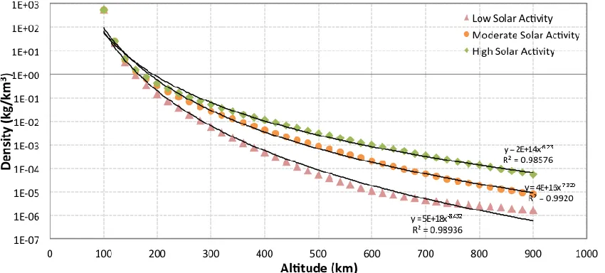
Curve fitting was used in (Reference 16) to produce power series’ to model atmospheric densi-ty at low, moderate and high solar actividensi-ty levels, resulting in the curves shown in Figure 1. These curves were produced using the Committee on Space Research International Reference Atmos-phere, commonly known as CIRA or CIRA-2012.20

Figure 1 – Power curve fit for various solar activity levels (N.B. logarithmic y-axis)

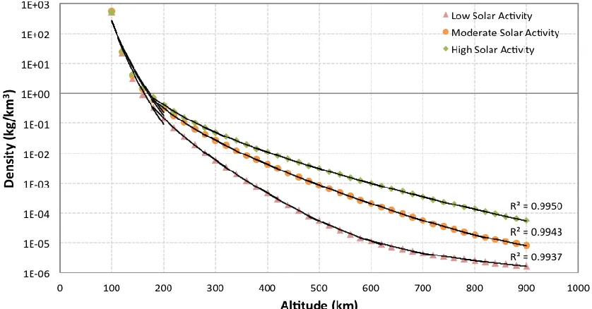
Figure 2 – Power Curve Segmented Fit for various solar activity levels (N.B. logarithmic y-axis)

This approach produces a much more accurate fit over the entire data set however it can be seen in Figure 2 that the transition between curves at lower altitudes is problematic. As such, the curves are extended to find the point of intersection and this point is then used as the transition to avoid discontinuities in the model. The improvement in accuracy provided by single curves ver-sus multiple curves is slight when considering the R2 values. However, as will be seen the im-provement in the lifetime predictions is notable.

MODEL VALIDATION USING HISTORICAL DATA

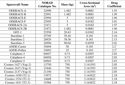
Table 1 – Validation Mission Spacecraft Characteristics; data from (References 21, 22 & 23)

Spacecraft Name NORAD

Catalogue No. Mass (kg)

Cross-Sectional Area (m2)

Drag Coefficient

ODERACS-A 22990 1.482 0.0081 1.93

ODERACS-B 22991 1.482 0.0081 1.99

ODERACS-E 22994 5 0.0182 1.96

ODERACS-F 22995 5 0.0182 2.01

ODERACS-2A 23471 5 0.0182 1.97

ODERACS-2B 23472 1.482 0.0081 1.96

GFZ-1 23558 20.63 0.0362 2.16

Starshine-1 25769 39.46 0.181 2.16

Starshine-2 26929 38.56 0.181 2.15

Starshine-3 26996 90.04 0.6939 2.01

ANDE-Castor 35694 50 0.183 2.2*

ANDE-Pollux 35693 25 0.183 2.2‡

Calsphere-3 04957 0.73 0.0507 2.03

Calsphere-4 04958 0.73 0.0507 2.03

Calsphere-5 04963 0.73 0.0507 2.03

Cosmos 1427 (Yug-2) 13750 750 3.141593 2.05

Cosmos 1615 (Yug-3) 15446 750 3.141593 2.05

Cosmos 2137 (Yug-4) 21190 750 3.141593 2.05

Cosmos 1450 (T2-1) 13972 750 3.163622 2.18

Cosmos 1534 (T2-2) 14668 750 3.163622 2.18

Cosmos 1631 (T2-3) 15584 750 3.163622 2.18

Each of the satellites in Table 1 are spherical, allowing simplification in the initial stages of model development as it allows the removal of attitude awareness problem. Attitudes of a decay-ing spacecraft can be difficult to predict, as most will have lost power by re-entry they are unable to maintain a steady attitude and will tumble, altering the drag coefficient and cross-sectional ar-ea, and complicating the analysis. However, satellites with non-uniform cross-sectional areas could be analyzed using the ISO (International Organization for Standardization) Standard for averaging the cross-sectional area; the standard also provides direction on estimating the drag coefficient, for use with spacecraft for which this is uncertain.24

RESULTS

Modified King-Hele Method Validation

The Modified King-Hele Method was applied to the missions detailed in Table 1 to test the accuracy of lifetime predictions produced.

*

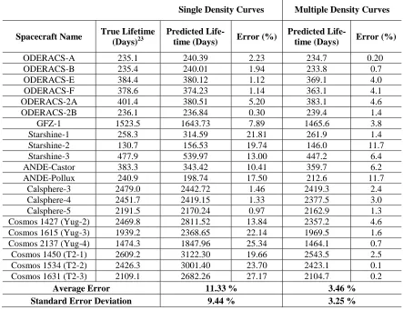
Table 2 – Lifetime Analysis Results vs. True Lifetimes of Validation Missions

Single Density Curves Multiple Density Curves

Spacecraft Name True Lifetime (Days)23

Predicted

Life-time (Days) Error (%)

Predicted

Life-time (Days) Error (%)

ODERACS-A 235.1 240.39 2.23 234.7 0.20

ODERACS-B 235.4 240.01 1.94 233.8 0.7

ODERACS-E 384.4 380.12 1.12 369.1 4.0

ODERACS-F 378.6 374.23 1.14 363.1 4.1

ODERACS-2A 401.4 380.51 5.20 383.1 4.6

ODERACS-2B 236.1 236.84 0.30 239.4 1.4

GFZ-1 1523.5 1643.73 7.89 1465.6 3.8

Starshine-1 258.3 314.59 21.81 261.9 1.4

Starshine-2 130.7 156.53 19.74 146.0 11.7

Starshine-3 477.9 539.97 13.00 447.2 6.4

ANDE-Castor 383.3 343.42 10.41 359.7 6.2

ANDE-Pollux 240.9 198.74 17.50 212.6 11.7

Calsphere-3 2479.0 2442.72 1.46 2419.3 2.4

Calsphere-4 2451.7 2419.15 1.33 2377.5 3.0

Calsphere-5 2191.5 2170.24 0.97 2162.9 1.3

Cosmos 1427 (Yug-2) 2469.8 2811.52 13.84 2357.2 4.6

Cosmos 1615 (Yug-3) 1939.2 2368.65 22.14 1969.5 1.6

Cosmos 2137 (Yug-4) 1474.3 1847.96 25.34 1464.1 0.7

Cosmos 1450 (T2-1) 2609.2 3122.30 19.66 2543.5 2.5

Cosmos 1534 (T2-2) 2426.3 3001.40 23.70 2423.1 0.1

Cosmos 1631 (T2-3) 2109.1 2682.26 27.17 2104.7 0.2

Average Error 11.33 % 3.46 %

Standard Error Deviation 9.44 % 3.25 %

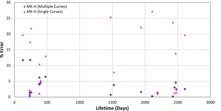
It is seen in Table 2 that using the multiple curves from Figure 2 to model atmospheric density produces more accurate results. Comparing the average error it is seen that in using multiple curves to model atmospheric density the method produces errors much smaller than those pro-duced by the same method incorporating the single atmospheric density curves from Figure 1. This can be attributed to the marked increase in accuracy of the density model; in some cases the single curve density was an order of magnitude different to the multiple curve density.

Figure 3 - Modified King-Hele Method Validation

When considering the validation results graphically it becomes clear that the largest errors in the multiple curve method tend to occur in the lowest lifetime missions. This further suggests that the method is practically sound, given that the method is far more sensitive to uncertainty in the input parameters for shorter missions, therefore these anomalies could be accounted for in this way. For example there may have been a short spike in solar flux, which over longer lifetime would have averaged out but would cause a greater uncertainty in the density, which in turn would produce greater errors in the shorter lifetime. Applying a Monte-Carlo analysis, and vary-ing the solar conditions input would address this uncertainty.

COMPARISON TO OTHER METHODS

To further verify the Modified King-Hele method it has been tested against other available methods, including the original King-Hele method,1,2 the Griffin & French method,4 and third-party, occasionally commercial, tools.

Third- Party Software

Many examples of third party software for orbit propagation and lifetime estimation exist however the three most notable are DAS by NASA, QProp by 1Earth and STK by AGI.

Debris Assessment Software (NASA). DAS uses the various propagators accounting for all

sig-nificant perturbing forces however it neglects to include an accurate coefficient of drag, instead assuming a standard coefficient of 2.2. The coefficient of reflectivity is also set as 1.25. These set parameters can introduce significant inaccuracies therefore it is not considered for comparison to the Modified King-Hele method.25

QuickProp (1Earth). QProp uses a semi-analytical propagation procedure based on the mean

orbit elements, therefore it is likely not the most accurate representation of a propagation soft-ware. Also data is not readily available on the intricacies of the model therefore this model is not considered for comparison either.26

Systems Tool Kit (AGI). Systems Tool Kit from AGI, often referred to as STK, is a software

that allows users to build and analyze virtual models of complex space systems with

time-0 5 10 15 20 25 30

0 500 1000 1500 2000 2500 3000

%

E

rr

o

r

Lifetime (Days)

tions algorithm to compute the expected lifetime of a satellite based on atmospheric drag.27 The lifetime analysis tool uses an algorithm which takes into account launch date, initial orbit, mass, cross-sectional area and drag coefficient. The algorithm then computes the effect of atmospheric drag using the satellite characteristics and atmospheric density and solar flux models chosen from several options. These options must all be considered to be sure the best available and most ap-propriate models are chosen.

Cojuangco examined the STK lifetime analysis tool to find that the NRLMSISE-00 density model was best suited to lifetime analysis in-order to minimize errors.28 The accuracy and speed of the analysis can be varied using the advanced options, which allow the time steps and the limit of the propagation to be set. As the speed was increased, the accuracy was decreased therefore a balance must be struck between the two.28 The propagator used in the analysis can also affect the results. Cojuangco found that the High Precision Orbit Propagator (HPOP) numerical propagator was the most accurate for lifetime analysis. HPOP numerically integrates the differential equa-tions of motion with a full range of perturbaequa-tions including gravitational models, third-body inter-actions, solar radiation pressure, and atmospheric drag. 28

STK was found to be the most promising of the three software choices considered. Therefore, it is used as a comparison to the Modified King-Hele method.

Method Comparison

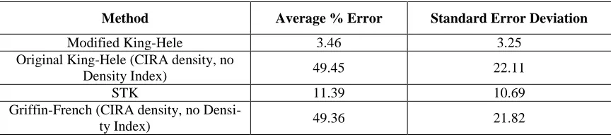
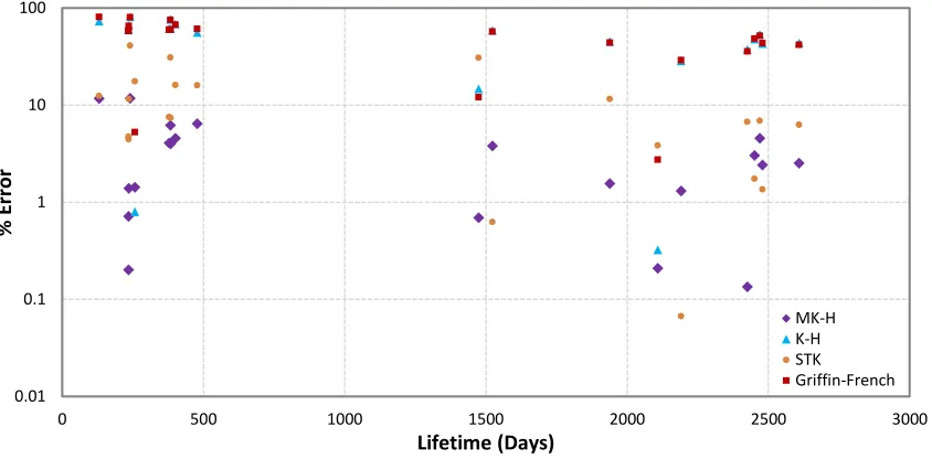
A lifetime analysis of each of the selected historical missions was completed using each of the comparison methods. The results are tabulated in Table 3 and plotted in Figure 4, which show the comparison of the Modified King-Hele method developed herein to the original King-Hele meth-od updated to include the CIRA density multiple curve mmeth-odel for average solar conditions (i.e. without the density index). Also included are the numerically produced STK model results for comparison. Finally included for comparison is the Griffin-French analytical method, which is similar to the original King-Hele method, and uses the CIRA density multiple curve model for average solar conditions to calculate lifetime using a standardized equation, however it’s deriva-tion limits its appropriate applicaderiva-tion to initially circular orbits.10

Table 3 – Comparison of Accuracy of Discussed Methods

Method Average % Error Standard Error Deviation

Modified King-Hele 3.46 3.25

Original King-Hele (CIRA density, no

Density Index) 49.45 22.11

STK 11.39 10.69

Griffin-French (CIRA density, no

Figure 4 – Accuracy Comparison of Discussed Methods (N.B. logarithmic y-axis)

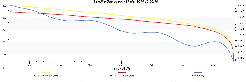
Table 3 shows that the modified King-Hele method produces the most accurate results. It is the only method that produces an average error of less than 10% including standard deviation; the next best method is STK, which has an average error of 11.4% and a standard deviation of 10.7%. Over the lifetime the perigee, apogee and eccentricity can be predicted to determine how the spacecraft deorbits; Figure 5 shows the results for one of the test cases, ODERACS-A, produced by the Modified King-Hele method while Figure 6 shows the results produced by STK.

Figure 5 – Modified King-Hele Method Orbit Decay Projected Progression of ODERACS-A

0.01 0.1 1 10 100

0 500 1000 1500 2000 2500 3000

%

E

rr

o

r

Lifetime (Days)

MK-H K-H STK Griffin-French

0 50 100 150 200 250

0 100 200 300 400

Time (days)

Altitud

e (k

m)

Oderacs-A

0 50 100 150 200 2500

1 2 x 10-3

Ecc

entri

city

Figure 6 – STK Orbit Decay Projected Progression of ODERACS-A

While the projected progression of the decay in the height of perigee and apogee match be-tween the two methods, the projected progression of the eccentricity is different. This difference is due to the STK solution being a numerical solution while the Modified King-Hele method is an average solution.

MONTE CARLO ANALYSIS

A major benefit of the Modified King-Hele Method is that a Monte Carlo Analysis can be ap-plied to it without drastically increasing the time taken to solve in relation to the time it takes to produce a similarly accurate numerical solution. While numerical solvers can take minutes to days to find just one solution, depending on the hardware and solution accuracy employed, the Modified King-Hele method took 8.5 seconds to run a Monte-Carlo analysis, of 210000 simula-tions, on the historical missions selected for validation. This test was done using MATLAB R2014a on a standard Windows 7 desktop computer, with an Intel i7-3770 @ 3.4 GHz with 8 cores and 16384 MB of RAM.

This offers a user the chance to see how the variation in parameters such as the initial eccen-tricity, the spacecraft mass or even the launch date will vary the lifetime produced. A Monte-Carlo analysis can also be used to provide confidence in the predicted lifetime by accounting for errors introduced by including variations in parameters such as solar flux thereby producing max-imum and minmax-imum bounds for a mission. The probabilities produced by the Monte Carlo analy-sis can then be fed into higher levels of analyanaly-sis, such as estimating mission costs or regulatory compliance checks.

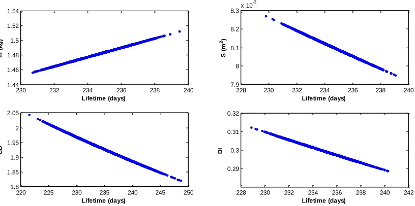
Figure 7 – Monte-Carlo Analysis of ODERACS-A Lifetime – Effects of Variations in Individual Pa-rameters

It can be seen that while the mass is directly proportional to the lifetime (increasing the mass while holding the other parameters constant will increase the lifetime), the cross-sectional area, and drag coefficient are both indirectly proportional. The relationship between the density index and lifetime is more complex, however there is a strong inverse correlation. It is seen here to have a relatively linear relationship, however this is not always the case. These relationships are as ex-pected as increasing the mass, and or decreasing the drag coefficient, and or the cross-sectional area will increase the potential forward momentum of the spacecraft leading to an increased life-time. Also a decrease in the density index implies a decrease in atmospheric density, which would lead to a longer lifetime.

Figure 8 – Monte-Carlo Analysis of ODERACS-A Lifetime – Probability Distributions Showing the Effects of Variations in Individual Parameters

230 232 234 236 238 240 1.44 1.46 1.48 1.5 1.52 1.54 Lifetime (days) m ( k g )

228 230 232 234 236 238 240 7.9

8 8.1 8.2 8.3x 10

-3 Lifetime (days) S ( m 2)

220 225 230 235 240 245 250 1.8 1.85 1.9 1.95 2 2.05 Lifetime (days) CD

228 230 232 234 236 238 240 242 0.29 0.3 0.31 0.32 Lifetime (days) DI

230 232 234 236 238 240 0 5 10 15 20 25 Lifetime (days) P ro b a b il it y ( % ) m

230 232 234 236 238 240 0 5 10 15 20 25 Lifetime (days) P ro b a b il it y ( % ) S

220 225 230 235 240 245 250 0 5 10 15 20 25 Lifetime (days) P ro b a b il it y ( % ) Cd

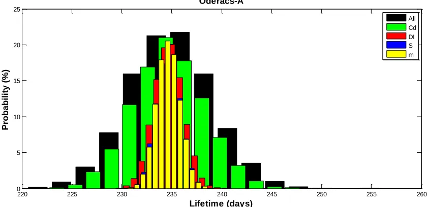
It should be noted that the launch date is actually a secondary parameter as it informs the den-sity index, which then directly affects the predicted lifetime. These individual variations can then be overlaid, as seen in Figure 9.

Figure 9 – Monte-Carlo Analysis of ODERACS-A Lifetime – Overlay of Individual Parameter Varia-tions Probability DistribuVaria-tions

This overlay highlights the effect that, for this case, the uncertainty in drag coefficient pro-duced the largest uncertainty in the lifetime predicted, while the uncertainty in mass propro-duced the smallest uncertainty in predicted lifetime. This can be attributed to the percentage error applied due to the directly proportional relationship between mass and lifetime. However upon examina-tion of the spread produced by the density index and drag coefficient, both of which had the same percentage error estimation it becomes clear that variations in the density index has a much smaller effect on the lifetime of this spacecraft due to the complex nature of it relationship to life-time.

For non-spherical spacecraft the cross-sectional area can be calculated based on the dimen-sions of the spacecraft and the projected tumbling mode. However, without knowing for certain how the spacecraft will tumble the area can only be determined with a degree of accuracy there-fore it is recommended to find a best case scenario and a worst case scenario to provide informed bounds for a Monte-Carlo simulation. Alternatively the ISO standard, with an estimated 20% er-ror, may be used. It should be noted though that this standard was originally created using a flat plate model, therefore it may not be the best representation of a specific spacecraft.

The density index cannot be directly measured rather it is inferred. It is recommended that in this case a fixed percentage error be applied to account for the largest range of possible errors. In the test cases a standard 5% error in the density index was assumed to produce the bounds for the Monte-Carlo simulation, however in some cases this error could be reduced or increased. For

ex-220 225 230 235 240 245 250 255 260

0 5 10 15 20 25

Lifetime (days)

Pr

ob

ab

ilit

y (

%)

Oderacs-A

Figure 9 shows that the lifetime is likely around 235 days, as also shown in Table 2, with a standard deviation of approximately 4 days. This means that the probability of the actual lifetime being in the range 231-239 days is approximately 68% (1σ), whilst the probability of the actual lifetime being in the range 227-243 days is approximately 95% (2σ) and the probability of the actual lifetime being in the range 223-247 days is approximately 99.7% (3σ); the actual lifetime of ODERACS-A was in fact 235 days. By improving the knowledge behind the estimation of pa-rameters, the standard deviation can be decreased and therefore the lifetime ranges produced can be narrowed.

Confidence intervals can be applied to the entire set of validation missions to further demon-strate the accuracy of the Modified King-Hele method. The 95% confidence interval can be seen in Figure 10, and the 99.7% confidence intervals can be seen in Figure 11.

Figure 10 – Monte-Carlo Analysis of all Validation Missions (red markers – true lifetime, blue mark-ers – predicted lifetime with attached 95% confidence interval)

Figure 11 – Monte-Carlo Analysis of all Validation Missions (red markers – true lifetime, blue mark-ers – predicted lifetime with attached 99.7% confidence interval)

0 500 1000 1500 2000 2500 3000

0 5 10 15 20 25

Lifetime (days)

Er

ror

(%)

0 500 1000 1500 2000 2500 3000

0 5 10 15 20 25

Lifetime (days)

Er

ror

In both figures the blue ranges given are the confidence intervals, with blue markers represent-ing the mean values, whilst the red markers show the true lifetime of the spacecraft. It can be seen that in approximately three-quarters of cases the true lifetime falls within the 95% interval whilst in all but two cases the true lifetime falls within the 99.7% interval. The 2 cases that exceed the 3σ interval are the same 2 missions that have errors above 10%, they are both short lifetimes therefore though they fall outside of the interval the difference between the mean and the true lifetime is within 15 days.

CONCLUSION

The Modified King-Hele method has been shown to compare favorably to other analytical methods and third party tools producing a significantly lower average error, at 3.46% and stand-ard deviation of 3.25%. It has also been shown that the modifications made to the original King-Hele method updated with CIRA density data reduced the average error from 49.45%; down roughly 14 times. Notably, STK produced predictions with an average error of 11.39% with standard deviation 10.69%.

The Monte-Carlo analysis that can be swiftly produced allows considerable confidence to be placed in the result. Whilst any special perturbations method can produce acceptable results, the overall process would be more costly.

REFERENCES

1

Cook, G. E., King-Hele, D. G., and Walker, D. M. C., “The Contraction of Satellite Orbits under the influence of Air Drag,” Proceedings of the Royal Society A: Mathematical, Physical and Engineering Sciences, vol. 257, 1960, pp. 224–249.

2

King-Hele, D. G., Satellite Orbits in an Atmosphere: Theory and Application, Springer Science & Business Media, 1987.

3

King-Hele, D. G., and Walker, D. M. C., The Prediction of Satellite Lifetimes, Royal Aircraft Establishment, Technical Report 87030, Farnborough: 1987.

4

Griffin, M. D., and French, J. R., Space Vehicle Design, Reston VA: American Institute of Aeronautics and Astronautics, Inc., 2004.

5

Xu, G., Tianhe, X., Chen, W., and Yeh, T.-K., “Analytical solution of a satellite orbit disturbed by atmospheric drag,” Monthly Notices of the Royal Astronomical Society, vol. 410, Jan. 2011, pp. 654–662.

6 _{Schatten, K. H., “Solar activity and the solar cycle,”}

Advances in Space Research, vol. 32, Aug. 2003, pp. 451–

460.

7

Schatten, K., Long-Range Solar Activity Predictions: A Reprieve From Cycle #24’s Activity, 2003.

8 _{Schatten, K., “Fair space weather for solar cycle 24,”}

Geophysical Research Letters, vol. 32, 2005, p. L21106.

9

Schatten, K., and Pesnell, W. D., Solar cycle #24 and The Solar Dynamo, 2007.

10 _{Berry, K., and Schatten, K., “Orbit decay prediction sensitivity to solar flux variations,”}

AIAA/AAS

Astrrodynamics Specialist Conference, Mackinac Isl: 2008, pp. 1–19.

11 _{Dikpati, M., and Gilman, P. A., “Simulating and Predicting Solar Cycles Using a Flux Transport Dynamo,”}

The

Astrophysical Journal, vol. 649, Sep. 2006, pp. 498–514.

12 _{Vallado, D. A., and Finkleman, D., “A critical assessment of satellite drag and atmospheric density modeling,”}

Acta Astronautica, vol. 95, 2014, pp. 141–165.

13 _{Stewart, J. Q., and Panofsky, H. A. A., “The Mathematical Characteristics of Sunspot Variations,”}

The

Astrophysical Journal, vol. 88, 1938, pp. 385–407.

18 _{Steering Group and Working Group 4, “IADC Space Debris Mitigation Guidelines (Revision 1),” 2007, pp. 1–10.} 19

ECSS Requirements & Standards Devision, Space Product Assurance: Safety, Noordwijk: 1996.

20

Commitee on Space Research, COSPAR International Reference Atmosphere - 2012, 2012.

21 _{Bowman, B. R., and Moe, K., “Drag Coefficient Variability at 175-500 km from the Orbit Decay Analyses of}

Spheres,” AAS/AIAA Astrodynamics Conference, South Lake Tahoe, California: 2005, pp. 117–136.

22 _{Qi, Y., Li, H., Xiang, J., and Man, H., “Periodic Variations of Drag Coefficient for the ANDE Spherical Satellites}

During its Lifetime,” Chinese Journal of Space Science, vol. 33, 2013, pp. 525–531.

23 _{Kelso, T. S., “CelesTrak NORAD Two-Line Element Sets Historical Archives” Available:}

https://celestrak.com/NORAD/archives/ Accessed: November 2014.

24

International Organisation for Standardisation, 27852:2010(E): Space systems — Estimation of orbit lifetime, 2010.

25 _{NASA, “Debris Assessment Software,” 2012.}

26 _{Oltrogge, D. L., and Leveque, K., “An Evaluation of CubeSat Orbital Decay,”}

25th Annual AIAA/USU

Conference on Small Satellites, Logan: 2011.

27 _{AGI, “STK,” 2014.} 28