City, University of London Institutional Repository
Citation:
Baronchelli, A. and Loreto, V. (2006). Ring structures and mean first passage
time in networks. Physical Review E - Statistical, Nonlinear, and Soft Matter Physics, 73(2),
doi: 10.1103/PhysRevE.73.026103
This is the unspecified version of the paper.
This version of the publication may differ from the final published
version.
Permanent repository link:
http://openaccess.city.ac.uk/2670/
Link to published version:
http://dx.doi.org/10.1103/PhysRevE.73.026103
Copyright and reuse: City Research Online aims to make research
outputs of City, University of London available to a wider audience.
Copyright and Moral Rights remain with the author(s) and/or copyright
holders. URLs from City Research Online may be freely distributed and
linked to.
City Research Online:
http://openaccess.city.ac.uk/
[email protected]
arXiv:cond-mat/0501669v2 [cond-mat.stat-mech] 8 Feb 2006
Andrea Baronchelli and Vittorio Loreto INFM and Dipartimento di Fisica,
Universit`a di Roma “La Sapienza” and INFM Center for Statistical Mechanics and Complexity (SMC),
Piazzale A. Moro 2, 00185 Roma, Italy
(Dated: February 2, 2008)
In this paper we address the problem of the calculation of the mean first passage time (MFPT) on generic graphs. We focus in particular on the mean first passage time on a nodesfor a random walker starting from a generic, unknown, nodex. We introduce an approximate scheme of calculation which maps the original process in a Markov process in the space of the so-called rings, described by a transition matrix of size O(lnN/lnhki ×lnN/lnhki), where N is the size of the graph and hkithe average degree in the graph. In this way one has a drastic reduction of degrees of freedom with respect to the size N of the transition matrix of the original process, corresponding to an extremely-low computational cost. We first apply the method to the Erd¨os-Renyi random graph for which the method allows for almost perfect agreement with numerical simulations. Then we extend the approach to the Barabasi-Albert graph, as an example of scale-free graph, for which one obtains excellent results. Finally we test the method with two real world graphs, Internet and a network of the brain, for which we obtain accurate results.
PACS numbers: PACS: 89.75.Hc, 05.40.Fb, 05.60.Cd
I. INTRODUCTION
Modern graph theory starts with the study of Erd¨ os-Renyi random networks in 1959 [1]. In more recent times it has regained a great amount of attention [2] since it has become evident that many different system can be described as complex scale free networks i.e assemblies of nodes and edges with nontrivial topological proper-ties [3, 4].
In this article we focus on the properties of random walks on generic graphs. It is well known that random walk is a fundamental process to explore an environ-ment [5, 6, 7, 8, 9, 10], and recently great attention has been devoted to the study of random walk on networks (see, for instance, [11, 12, 13, 14, 15, 16, 17, 18, 19, 20]). In this process a walker, situated on a given node at time
t, can be found with probability 1/k on any of the k
neighbors of that node at timet+ 1.
In particular we are interested in the mean first passage time (MFPT) on a nodesfor a random walker starting from a generic, unknown, nodex. It is important to note here that Noh and Rieger [14] have derived, exploiting the properties of Markov chains, an exact formula for the MFPTTsj of a random walker between two nodess
andj in a generic finite network.
In this paper, however, we do not trivially average Tsj
over all j 6= s, a very costly operation, but we use the concept of ring (see also [21]). In this perspective we study the graph as seen by node s, and partition it in rings according to the topological distance of the dif-ferent nodes from s (see also [16, 22]). This allows us to map the original Markov problem (of N states) in a new Markov chain of drastically reduced dimension (O(lnN/lnhki ×lnN/lnhki)) and, as a consequence, to calculate MFPT on a generic nodeswith a reduced
com-putational cost. On the other hand with the new process the identity of the single target nodesis lost, and all the nodes with the same connectivity (i.e. number of neigh-bors) are not distinguishable.
Our explicit calculation is almost free of approximations only for Erd¨os-Renyi random graphs, for which we obtain an excellent agreement between theory and numerical simulations. The more disordered scenario of other com-plex networks makes the extension of our approach pro-gressively more problematic. Nevertheless we find quite surprisingly that our approach is able to make very good predictions also for other synthetic networks, such as the Barabasi-Albert scale free networks [23], and at least two real world graphs. In all these cases, the considered net-works behave, with respect to the property studied, as if they were random graph with the same average degree. Finally our approach allows us to show that a random walker recovers rapidly the degree distribution of the net-work it is exploring.
2
II. THE NEW PROCESS - RINGS
All the information about a generic graph is contained in the adjacency matrixAwhose elementAij = 1 if nodes
i andj are connected, andAij = 0 otherwise. We shall
consider here only undirected graphs, i.e. Aij = Aji,
which do not contain any links connecting a node with itself (Aii = 0, ∀i). The degree of a node,k(i), is given by
k(i) =P
jAij. Finally, we shall concentrate only on the
case of connected graphs, i.e. graphs in which each pair of nodes i, j, withk(i), k(j)6= 0, are connected with at least one single path. From a random walk point of view the matrixAcan be interpreted as theN×N symmetric transition matrix of the associated Markov process [32].
We are interested in the problem of the average MFPT on a nodesof degreek(s) of a random walker that started from a different, unknown, nodex. Our idea is mapping the original Markov processAon a much smaller process
B which will be asymmetric and will contain self-loops (i.e. Bii 6= 0). More precisely we reduce the N ×N
matrix to aO(lnN/lnhki ×lnN/lnhki) matrix.
Given the target node s, we start by subdividing the entire network in subnetworks, orrings(see also [16, 22]),
rl, with the following property:
rl={nodes j|dsj=l} (1)
where dsj =djs is the distance between nodess andj,
i.e. the smallest number of links that a random walker has to pass to get from j to s. These rings will be the states of the new matrixB. Their number, being propor-tional to the maximum distance between any two nodes in the network, i.e. to the diameter of the network, is
O(lnN/lnhki) [24, 25] (where hki is the average degree of the nodes of the graph).
Other important quantities are the average number
mrl,rl+1≡ml,l+1of links that connect all the elements of
rlwith all the elements ofrl+1, and the average number
ml,lof links between nodes belonging to the samerl. We
have triviallyml,l−1=ml−1,l andml,k= 0 ifdlk >1.
We now have all the elements to define our new process. We are no more interested in the exact position of the random walker. The relevant information is now the ring in which the random walker is. The matrix of this process has size (lmax+ 1)×(lmax+ 1), wherelmax is the
diam-eter of the original graph. The matrix has the following structure [33] (for the caselmax= 6):
B =
0 0 0 0 0 0 0
b10 b11 b12 0 0 0 0
0 b21 b22 b23 0 0 0
0 0 b32 b33 b34 0 0
0 0 0 b43 b44 b45 0
0 0 0 0 b54 b55 b56
0 0 0 0 0 b65 b66
(2)
where bij = mij/(Pl
max
k6=i=0mik + 2mii) for i 6= j, and
0.5 1 1.5 e 0.5 1 1.5 e
0 2 4 6 8
l 0 200 400 nl simulation theory
0 2 4 6 8
l 0 200 400 nl 0 200 400 nl l 0 200 400 nl
0 2 4 6 8
l
0.5 1
e
0 2 4 6 8
[image:3.612.324.554.47.229.2]l 0.5 1 e k(s)=2 k(s)=4 k(s)=6 k(s)=8
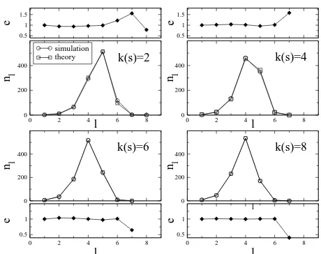
FIG. 1: Nodes nl per ring: Rings populations nd are
shown in this figure. Comparisons of theoretical previsions from eq.(6) and data from simulations for different values of
k(s) in a single E-R graph of size N = 103 andhki = 6 are
shown. The fractional errore, defined as the ratio between measured and calculated values, is also plotted for each rep-resented value ofk(s). Theoretical average quantities are in excellent agreement with single graph measurements.
bii= 2mii/(Pl
max
k6=i=0mik+ 2mii). bij thus represents the
probability of going from ringito ringj. By definition of rings it is clear that it is not possible to move from a ring to a non-adjacent other ring, while it is obviously possible to move inside a ring, and in this case the number of links must be doubled to take into account that each internal link can be passed in two directions. The elements of the first row of the matrix are set equal to 0 because we are interested in thefirst passage time in the target nodes. The probabilityPij(t)of going from stateito statej in t
steps is given by (Bt)
ij. If we setb01= 1, we would allow the walker to escape from nodes, while b00 = 1 should be used if we were interested in the probability that the walker reached node s before time t. The probability
Fk(s)(t) that thefirst passage on nodesoccurs at time t is then:
Fk(s)(t) =
lmax
X
l=1
nl
N−1 (B
t)
l0 (3)
where nl is the number of nodes belonging to the ring
rland each matrix term is weighted with the probability
that the random walker started in the ring corresponding to its row, i.e. nl/(N−1).
The average time MFPTτ(k(s)) can be calculated using eq.(3) as:
τ(k(s))) = ∞
X
l=1
0 2 4 6 8 l
2 4 6 8 10 12
<k(r
l
)>
[image:4.612.64.291.51.212.2]k(s)=2 k(s)=4 k(s)=6 k(s)=8 k(s)=10 k(s)=12 theory k(s)=6
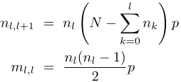
FIG. 2: Average ring degree: average degrees of nodes be-longing to different rings are shown in function of rings’ dis-tances for an ER random graph (N = 104nodes andhki= 6).
A dependence on ring’s distance appears clearly, as predicted by theory. Results for different values ofk(s) are shown (pre-dictions shown only for the casek(s) = 6).
III. EXPLICIT CALCULATION FOR RANDOM
GRAPHS
A. Static
A random graph is obtained in the following manner: given a finite set of isolatedNnodes, all theN×(N−1)/2 pairs of nodes are considered and a link between two nodes is added with probability p. This yields (in the limitN → ∞) to Poisson’s distribution for the degreek
of a node:
P(k) =hki
k
k! e
−hki (5)
with hki=p(N −1). It is clear that such a graph does not contain any relevant correlations between nodes and degrees, and this will allow us to obtain exact average relations for the quantities illustrated in the previous sec-tion.
The first important quantity to calculate is the average numbernl of elements ofrl. It holds
nl+1= N−
l X
k=0
nk !
(1−(1−p)nl
) (6)
wherenl+1is calculated as the expected number of nodes not belonging to any interior ring that are connected with at least a member of rl. Figure 1 illustrates that eq.(6)
is in excellent agreement with results from simulations. Obviouslyn0 = 1 and n1 = hki. However, if we know the degreek(s) of node swe can impose n1=k(s) and calculate the followingnl>1in the usual manner. In fact, this is the way in which we will use eq.(6).
For the average numbersml,l+1 of links that connect all the elements ofrl with all the elements ofrl+1, and
ml,l of links between nodes belonging to the samerl we
have:
ml,l+1 = nl N−
l X
k=0
nk !
p (7)
ml,l =
nl(nl−1)
2 p
where the fact that a link between two nodes exists with probabilitypis exploited. As a practical prescription we add that when eq. (7) yields to non-physical ml,l < 0
one has to redefine ml,l = 0. Also these expressions,
which are crucial for the construction of the B matrix of eq. (2), give predictions in excellent agreement with results from simulations (data not shown). As expected we have that, in the limitp→0,ml,l+1 →nl+1, while, whenp→1,ml,l+1→nl×nl+1. Note that from eq. (7) one has that nl <1 ⇒ ml,l <0 which has clearly no
physical meaning.
Before going on it is interesting to make a remark. It is known [22, 27] that the nearest neighbors of a generic node have particular properties, e.g. an average degree different from the hki of the graph. Our relations are able to predict this fact. Combining eq.(6) and eq.(7) it is easy to see that the average degree of the nodes be-longing to rl depends on l, being constant (and larger
thanhki) for low values ofl and decreasing rapidly forl
large enough. Data from simulation reported in Figure 2 show that this prediction is correct. This agreement is not surprising since eq.(6) and (7) are separately in ex-cellent agreement with simulations, thus being able to predict very accurately the value of the average degree of the nodes belonging to the same ring.
B. Dynamics
So far, we have shown that predictions of the above relations on the static properties of a random graph are correct. We now explore the predictions on the diffu-sion processes. Figure 3 shows, for different values of the degree k(s) of the target node, the comparison of the predicted values of Fk(s)(t), calculated with eq.(3) and results from simulations. Data from simulations are obtained by selecting randomly, for each of the approxi-matelyN ×N runs, one of the nodes of selected degree
k(s) present in the network to play the role ofs, and one of the remaining N −1 nodes to be the starting point of the random walker. The agreement between theory and simulations is very good. The exponential behav-ior, typical of finite ergodic Markov chains, has the form
[image:4.612.378.505.118.176.2]f(t) = (1/τ)exp(−t/τ).
4
0 5×10³
10-4
10-3
0 2×10⁴
4×10⁴
t
10-6
10-5
10-4
10-3
Fk(s)
(t)
[image:5.612.64.289.50.202.2]k(s)=1 k(s)=6 k(s)=11 theory
FIG. 3: First passage time distributions: FPT prob-ability distributions both measured and calculated for an ER graph with hki = 6 are presented for different val-ues of k(s). Theoretical predictions are in excellent agree-ment with data of random walk on a single graph. Theo-retical curves are obtained with eq.(3), and fit the relation
Fk(s)(t) = (1/τ)exp(−t/τ) withτ obtained with eq.(4). In
the inset the first part of the distribution is showed in more detail.
1 10
k(s)
103
104
τ
simulation theory
1 10
k(s) 1.00
1.05 1.10
e
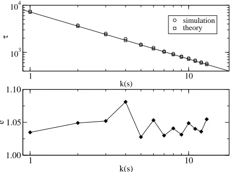
FIG. 4: Mean first passage times: in upper graph MFPT both measured and calculated (using eq.(4)) are reported for an ER graph of size N = 103 with hki = 6. Error bars on
measured values are not visible on the scale of the graph. The line τ(k(s)) ≃ τ(1)×k(s)−1 is also plotted. It holds τ(1)sim = 7413 andτ(1)calc= 7164 for values obtained
re-spectively from simulations and from calculation. It can be noted that the order of magnitude of τ(1) is given by 2M, whereM is the total number of links in the graph; in our case we have 2M≃ hki ×N = 6000. In lower graph the fractional errore, defined as the ratio between simulated and calculated MFPTs, is reported.
with those obtained in simulations. We shall return to the origin of the small disagreement between theory and simulations at the beginning of the next section.
The relation, found both in theory and simulations (see
0 10000 20000 30000 40000 t
0.5 1.0 1.5
e
0 10000 20000 30000 40000 10-8
10-7 10-6 10-5 10-4 10-3
P(t)
[image:5.612.325.556.50.207.2]theory simulation
FIG. 5: First passage time distribution - Average on
all target nodes s: The distribution of the FPT obtained
is shown (ER graph: N = 103,hki = 6). At each run both
the target nodesand the starting node of the random walker are randomly chosen. This means that in this distribution the degree of the target nodes is no more fixed. The non exponential curve is the result of the convolution of several exponential curves obtained for fixedk(s). The theoretical curve, obtained according to eq.(8), is in excellent agreement with data from simulation performed on a single graph. The fractional errore, defined as the ratio between simulated and calculated data, is also plotted. For large times poor statistics causes bigger fluctuations ofe.
also [14]),τ(k(s)) =τ(1)×k(s)−1, can be explained with elementary qualitative probabilistic arguments. In fact, since, as shown in Figure 2, the average degree of the nodes inr1 does not depend onk(s) (i.e. on the sizen1 of r1), also the MFPT on a node of r1 is independent fromn1. This means that, while the probability of pass-ing fromr1 to s does not depend on n1, a larger r1 is visited more often than a smaller one. Combining these observations, it seems plausible guessing that the MFPT on a target nodes with k(s)>1 will be 1/k times the MFPT of a nodeswithk= 1, and this behavior is indeed observed.
It is worth noting that both the k(s)−1 trend and the order of magnitude of τ(1) can be derived with a simple mean field approach [18, 19]. In fact, once neglected all the possible correlations in a graph, the whole random walk process can be approximated with a two state Markov process where the two states cor-respond to the walker being at the target node and on any other node. Easy calculations shows that the prob-ability for the walker to arrive at a node s is given by
q(s) =q(k(s)) =k(s)/2M, whereM is the total number of links of the graph. For a fully connected graph this relation gives the exact value ofτ=τ(N−1) =N−1. In a random graph the mean field approach gives bet-ter and betbet-ter results the larger is the mean degreehki. For small values ofhki, only the order of magnitude of
[image:5.612.64.293.340.509.2]based on rings, thought being less simple, is able to make more accurate predictions for all values of hki. Just for comparison we report here data shown in Figure 4 rela-tive to a network of N = 103 nodes with hki = 6 : we have τ(1)sim/τ(1)calc = 1.03 and τ(1)sim/2M = 1.24,
where τ(1)sim and τ(1)calc are MFPT obtained
respec-tively with simulations and with the ring method. All the results discussed above allow us to explain the curve presented in Figure 5, which represents the distri-bution P(t) of the MFPT in a graph when both s and the starting point of the walker are randomly chosen at each run. P(t) can be calculated here as the convolution of several exponential FPT distributions Fk(s)(t) corre-sponding to the different values of k(s), each weighted with the probability of encountering a node of degree
k(s) in the graph. More precisely, according to eq.(5), for each time stepteveryFk(s)(t) must be weighted with Poisson’s weightsc(kh(ksi))= hki
k(s)
k(s)! e−hki. We have:
P(t) = ∞
X
j=1
c(jhki)Fj(t)
= ∞
X
j=1
c(jhki)e(−t/τ(j))
1
τ(j) (8)
This relation can be written in a more compact way ex-ploiting the fact that τ(k(s)) =τ(1)×k(s)−1 [26]. De-finedZ=hki ×exp(−t/τ(1)), it holds:
P(t) = ∞
X
j=1
Z Z
j−1
(j−1)!
e−hki
τ(1) =cZe
Z (9)
wherec is the constant eτ−h(1)ki.
IV. EXTENSIONS OF THE THEORY
In the previous sections we have described a method that allows to calculate the average MFPT on a node s
of a walker that started from a generic other node of the graph. We have then obtained exact (average) expres-sions for the case of random graphs. Unfortunately, the analytical extension of the relations found for this kind of graphs to other graphs (such as, for example, scale free networks) is difficult. This is due to the fact that eq.(6) and eq.(7) exploit the knowledge of the rules ac-cording to which a random graph is generated. In other words the absence of correlations between nodes is the main feature those equations are based on. When corre-lations are present the calculation of the number of nodes of the second ring,n2, is already very difficult (for finite networks) and requires some empirical assumptions [27]. In addition there is a more subtle reason that makes our method difficult to extend. Given the set of all nodes of a graph with a certain degree k, their first rings, al-though having the same number of nodes, present two
0 5 10 15 20
<k(r
1)>
0 1000 2000
N(<k(r
1
)>)
Erdos-Renyi graph
10 100
<k(r
1)>
100
101
102
103
Barabasi-Albert graph
0 0.2 0.4 0.6 0.8 1
σ(r1)/k(r1)
0 200 400
Nσ
/k
0 0.5 1 1.5 2
σ(r1)/k(r1)
[image:6.612.324.553.51.238.2]0 500 1000
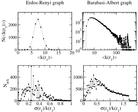
FIG. 6: First ring fluctuations: Fluctuations related to nodes of degree k = 3 are presented for ER (left) and BA (right) graphs of sizeN = 1×10⁵ andhki= 6. On the two
top figures global fluctuations are analyzed. Histograms of the number of nodes vs. the average degreek(r1) of the nodes
of the first ring r1 for ER graphs (top-left) and BA graphs
(top-right). Logarithmic scale for the ordinate of BA graph must be noted. In the two bottom figures local fluctuations are analyzed. Here the histograms represent the number of rings in function of the ratioσ(r1)/k(r1), whereσ(r1) is the
variance of the degree of the nodes belonging to eachr1 for
ER graphs (top-left) and BA graphs (top-right). It is evident the higher degree of fluctuations of the BA graphs.
kinds of fluctuations. On a global scale, the average de-gree k(r1) of the nodes of the first ring does not have a unique value, but in general is distributed accord-ing to some probability density. On a local scale, on the other hand, a single ring is not made by identical nodes, and its average degree has a certain variance σ. In Figure 6 we show global and local fluctuations for both a random graph and a Barabasi-Albert (BA) scale free graph [23]. The preferential attachment rule of the Barabasi-Albert network generates a graph with a scale free formP(k)≃k−c, withc= 3, for the degree
distri-bution. As it is evident from Figure 6, BA graphs have larger fluctuations than random graphs.
6
0.0 3.0
100 101 102 103 102
103 104 105
MFPT
BA ER brain internet
100 101 102 103 k(s)
0.0 3.0 0.0 3.0
e
[image:7.612.62.292.49.215.2]k(s)
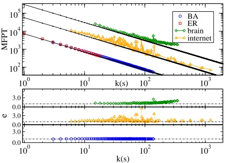
FIG. 7: Mean first passage times vs. the degree of
the target node for different networks. Continuous
lines with small filled points (upper graph) are obtained from eq.(4), i.e. for random ER graphs, while empty symbols of different shapes come from simulations. It is evident the ex-cellent agreement between theory and simulations both for ER graphs (circles) and, less obviously, for BA graphs (squares). Data from real networks are also reported: also in this case the agreement with theoretical predictions is good. Error bars are not visible on the scale of the graph. In lower graph frac-tional errors e, defined as the ratio between measured and calculated values, are reported both for real networks and BA graph. Dashed lines indicate correspond toe= 1.
for which our calculated MFPT are always smaller than those obtained from simulations.
Notwithstanding these difficulties in extending our the-ory, we found a quite surprisingly result, shown in Fig-ure 7: given a BA graph with a given average degreehki, the average MFPT for a walker starting from a generic node on a node s of degree k(s) is almost equal to the corresponding average MFPT of the same random walk on a random graph with the same average degree. This means that our theory continues to predict very well the MFPT (and hence its exponential distribution). It is re-markable that the theory predicts well also the MFPT on nodes with high degree, which are absent in the cor-responding random graph.
The ability of our theory to predict diffusion processes on BA graphs can be due to the modest presence of correlations between its nodes. Many properties of real networks, in fact, are not reproduced by the BA model. One important measure of correlations in a graph is the measure of the average degree of the nearest neighbors (i.e. of the nodes of the first ring) of vertices of degree
k, called knn [28]. While random and BA graphs have
a flat knn, indicating the absence of strong correlations
among nodes, many real networks exhibit either an as-sortative or disasas-sortative behavior. In the first case high degree vertices tend to be neighbors to high degree ver-tices, while in the second case they have a majority of low
degree neighbors. Another important measure of corre-lation is the clustering coefficient which is proportional to the probability that two neighbors of a given node are also neighbor of themselves. Again, BA and random graphs, in which clustering is very poor, do not reproduce the clustering properties of many real networks.
In order to check how far our theory can predict the MFPT on correlated graphs we have performed two sets of experiments on real networks. We have considered in particular a network of Internet at the level of Au-tonomous Systems [29, 30] which exhibits a disassorta-tive mixing feature and a recently proposed scale-free brain functional network [31] which exhibits an assor-tative mixing feature as well as a strong clustering coef-ficient.
The results for the MFPT for these two networks, as a function of the degree of the target node, are reported in Figure 7. Though the agreement between theory and simulation is not any more perfect, it remains good. In particular we find again the approximate trendτ(k(s)) =
τ(1)×k(s)−1.
Now we have all the elements to estimate the proba-bility of finding a random walker on a node of a given degreek. On the one hand, in fact, it seems obvious that this probability is related to the fractionf(k) of nodes of that degree in the network, while on the other hand we now know that the MFPT on such a node is propor-tional, on average, to 1/k. It is then reasonable arguing that the probability for a random walker being on a node of degreekis proportional to kf(k).
We have tested this hypothesis in an experiment reported in Figure 8. In the experiment a walker has explored a BA network and an ER random graph with N = 105 nodes for N time steps. At each time step the degree of the visited node was recorded and the normalized his-togram of the fraction of time spent on nodes of any de-gree is reported in Figure 8. In the limit of infinite time steps this histogram would indicate exactly the probabil-ity of finding the walker of a node of a givenk. According to our hypothesis, this histogram should be described by the functionP(k)k/hki, whereP(k) is the degree distri-bution of the considered network, and the Figure shows this is in fact the case, already after a relatively small number of time steps.
Finally, it is worth noting that the previous argument can be reversed. A walker able to record the degree of each node it traverses can be used to determine the degree distribution of the network it travels. In fact, ift(k) is the fraction of time spent on nodes of degreekit holds
f(k)∝t(k)/k. The average degree hki is then trivially obtained by requiring the normalization of the estimated
P(k).
V. CONCLUSIONS
100 101 102 103 k
10-4 10-3 10-2 10-1 100
t(k)
[image:8.612.65.290.53.211.2]BA graph P(k)*k/<k> (BA) ER graph P(k)*k/<k> (ER)
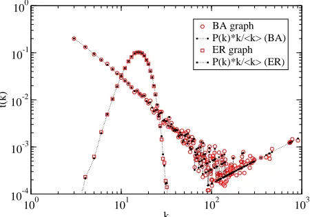
FIG. 8: Degree distribution exploration: a random walker explores the degree distribution of two networks: a BA graph of sizeN = 105 andhki= 6 and an ER random graph of sizeN = 105 andhki= 15. Simulations in which a walker
travels the networks forN time steps have been performed. Empty symbols in figure represent the fraction of time spent on a node of degree k. Filled symbols joined by light lines are obtained with the relationP(k)k/hki, where P(k) is the degree distribution of the considered network. Filled points fit well the experimental data, and, as it is obvious, a longer walking process would allow for better agreement. The prob-ability of finding a random walker on a node of a given degree
kis related to the degree distribution of the graph via the in-verse of 1/kMFPT scaling relation (apart from a normalizing factor). For BA graphs it holdsP(k)∝k−3. The first part
of the curveP(k)k/hkipresented in Figure is indeedc×k−2,
where cis a constant. The region of higher degrees, on the other hand, grows linearly due to the fact that in a finite size realization the statistics on high degree nodes is poor and the degree distribution in this region is flat. We avoided any bin-ning in experimental or theoretical data to make clear that the walker exploration of the network is not perfect.
s of random walkers starting from different nodes on a generic network. We have introduced a new approximate method, based on the concept of rings, which maps the original Markov process on another Markov process in a much smaller space. This allows for a drastic reduction of the computational cost. In the case of ER random graphs we have been able to analytically derive all the quantities of interest and we have shown that our method gives predictions, both for static and dynamic properties, in excellent agreement with results found in simulations. Even if this new method is promising, analytical results are difficult to obtain for non random graphs. However, quite surprisingly, we have found that MFPT calculated with our theory for ER graphs are in excellent agreement also with simulations of dynamics on BA networks and in good agreement with results obtained with random walkers on two real networks, thus making our method an easy tool to predict MFPT time related quantities in many cases. Acknowledgments: This research has been partly supported by the ECAgents project funded by the Future and Emerging Technologies program (IST-FET) of the European Commission under the EU RD contract IST-1940. The information provided is the sole respon-sibility of the authors and does not reflect the Commis-sion’s opinion. The Commission is not responsible for any use that may be made of data appearing in this publication. Brain data collection was supported with funding from NIH NINDS of USA (Grants 42660 and 35115). The authors are grateful to Claudio Castellano and Alessandro Taloni for many interesting discussions and Alain Barrat and Luca Dall’Asta for a careful read-ing of the manuscript.
[1] P. Erd˝os and A. R´enyi, Publ. Math. Debrecen 6, 290 (1959).
[2] B. Bollob´as,Modern Graph Theory(Springer, New York, 1998).
[3] R. Albert and A.-L. Barab´asi, Rev. Mod. Phys.74, 47 (2002).
[4] M. E. J. Newman,SIAM Review45, 167 (2003). [5] B. D. Hughes, Random Walks and Random
Environ-ments, (Clarendon Press, Oxford, 1996).
[6] S. Redner, A Guide to First-Passage Processes (Cam-bridge University Press, New York, 2001).
[7] L. Lov´asz, in Combinatorics, Paul Erd˝os is Eighty, Vol. 2 (eds. D. Mikl´os, V. T. S´os, T. Zs˝onyi), J´anos Bolyai Mathematical Society, Budapest, 1996, 353–398. [8] D. ben-Avraham and S. Havlin,Diffusion and Reactions
in Fractals and Random Systems, (Cambridge University Press, Cambridge, 2000).
[9] D. Aldous and J. A. Fill, Reversible Markov
Chains and Random Walks on Graphs.
http://stat-www.berkeley.edu/users/aldous/RWG/book.html. [10] W. Woess, Random Walks on Infinite Graphs and
Groups, (Cambridge University Press, Cambridge, 2000). [11] L. A. Adamic, R. M. Lukose, A. R. Puniyani, and B. A.
Huberman,Phys. Rev. E64, 046135 (2001).
[12] E. Almaas, R. V. Kulkarni and D.Stroud,Phys. Rev. E
68, 056105 (2003).
[13] M.E.J. Newman,Soc. Networks27, 39 (2005).
[14] J. D. Noh and H. Rieger, Phys. Rev. Lett. 92, 118701 (2004).
[15] L.K. Gallos,Phys. Rev. E70, 046116 (2004).
[16] V. Sood, S. Redner and D. ben-Avraham, J. Phys. A: Math. Gen.38109 (2005).
[17] E. M. Bollt and D. ben-Avraham, New J. Phys. 7, 26 (2005).
8
(2005).
[20] S.-J. Yang,Phys. Rev. E71, 016107 (2005).
[21] L. da F. Costa e-prints, arxiv:cond-mat/0408076 and arxiv:cond-mat/0412761.
[22] M.E.J. Newman,Social Networks25, 83-95 (2003). [23] A.-L. Barab´asi and R. Albert,Science286, 509 (1999). [24] F. Chung and L. Lu,Applied Math.26, 257 (2001). [25] F. Chung and L. Lu, Proc. Natl. Acad. Sci. 99, 15879
(2002).
[26] L. Dall’Asta,Private Communication(2005).
[27] M.E.J. Newman, in Handbook of Graphs and Networks, S. Bornholdt and H. G. Schuster (eds.), Wiley-VCH, Berlin (2003).
[28] R. Pastor-Satorras, A. Vazquez and A. VespignaniPhys.
Rev. Lett.87, 258701 (2001).
[29] Data have been downloaded from the site www.cosin.org. [30] R. Pastor-Satorras and A. Vespignani, Evolution and Structure of the Internet (Cambridge University Press, Cambridge, 2004).
[31] V.M. Egu`iluz, D.R. Chialvo, G.A. Cecchi, M. Baliki, and A.V. Apkarian,Physical Review Letters 94, 018102 (2005).
[32] A random walk can be seen as a Markov process with the identification position-state.