Time-frequency representation of earthquake accelerograms and inelastic structural response records using the adaptive chirplet decomposition and empirical mode decomposition

City, University of London Institutional Repository

Citation

:

representation of earthquake accelerograms and inelastic structural response records using the adaptive chirplet decomposition and empirical mode decomposition. Soil Dynamics and Earthquake Engineering, 27(7), pp. 675-689. doi: 10.1016/j.soildyn.2006.11.007

This is the unspecified version of the paper.

This version of the publication may differ from the final published

version.

Permanent repository link:

Link to published version

:

Copyright and reuse:

City Research Online aims to make research

outputs of City, University of London available to a wider audience.

Copyright and Moral Rights remain with the author(s) and/or copyright

holders. URLs from City Research Online may be freely distributed and

linked to.

City Research Online: http://openaccess.city.ac.uk/ [email protected]

Time- frequency representation of earthquake accelerograms and

inelastic structural response records using the adaptive chirplet

decomposition and empirical mode decomposition

Authors

P.D. Spanos1_,* _{A. Giaralis}2_{, N.P. Politis}3

Affiliations

1_{L. B. Ryon Chair in Engineering, Rice University, Houston, Texas}

2_{Ph.D. Candidate, Department of Civil Engineering, Rice University, Houston, Texas}

3_{Floating Systems Engineer, BP America Inc.}

Abstract

In this paper the adaptive chirplet decomposition combined with the Wigner-Ville

transform and the empirical mode decomposition combined with the Hilbert transform

are employed to process various nonstationary signals (strong ground motions and

structural responses). The efficacy of these two adaptive techniques for capturing the

temporal evolution of the frequency content of specific seismic signals is assessed. In this

respect, two near- field and two far- field seismic accelerograms are analyzed. Further, a

similar analysis is performed for records pertaining to the response of a 20-story steel

frame benchmark building excited by one of the four accelerograms scaled by appropriate

factors to simulate undamaged and severely damaged conditions for the structure. It is

shown that the derived joint time- frequency representations of the response time

* _{Pol D. Spanos, George R. Brown School of Engineering, L. B. Ryon Chair in}

Engineering, Rice University, MS 321, P.O. Box 1892, Houston, TX 77251, U.S.A.

histories capture quite effectively the influence of nonlinearity on the variation of the

effective natural frequencies of a structural system during the evolution of a seismic

event; in this context, tracing the mean instantaneous frequency of records of critical

structural responses is adopted.

The study suggests, overall, that the aforementioned techniques are quite viable

tools for detecting and monitoring damage to constructed facilities exposed to seismic

excitations.

Keywords: time-frequency representation; chirplets; empirical mode decomposition;

intrinsic modes; accelerograms; nonlinear structural response; damage detection

1. Introduction

Transient signals encountered in earthquake engineering and structural dynamics

are inherently nonstationary in the sense that both their frequency content and amplitude

vary with time. Typical earthquake accelerograms exhibit a time-evolving frequency

composition due to the dispersion of the propagating seismic waves, and a time-decaying

intensity after a short initial period of development. Structural systems are characterized

by their natural frequencies and modes of vibration, rendering their response to strong

ground motions a relative resonance phenomenon. Thus, capturing the time-varying

dominant frequencies present in a seismic accelerogram facilitates the assessment of its

structural damage potential. Furthermore, the time histories tracing certain structural

response quantities, such as floor displacements and inter-story drifts of a building under

evolving frequency content provides valuable information about the possible level of

global structural damage caused by the ground motion. Signals of this kind require a joint

time- frequency analysis.

Ordinary Fourier analysis has been used for several decades in earthquake

engineering for representing the frequency content of seismic events. In this regard there

are obvious limitations, since the Fourier transform can only provide an “average”

spectral decomposition of a signal. The availability of more powerful computers,

advances in applied mathematics [1-8], and the development of fast algorithms [7-12]

have facilitated the application of time-frequency analysis techniques in various

engineering fields over the past years. These techniques can be loosely divided into

adaptive and non-adaptive. It is the intention of this paper to exploit certain adaptive

methods for capturing the temporal variation of the frequency content of earthquake

accelerograms and of seismic structural response signals. However, it is emphasized that

techniques belonging to both the above categories constitute viable tools for the purpose.

To ensure completeness and to enhance the readability of the manuscript a

conspectus of the commonly used non-adaptive methods is first provided before focusing

on the adaptive methods that the present study considers.

Introduced by Gabor [13], the first and most widely used method for joint

time-frequency representation of non-stationary signals utilizes the so-called short-time

Fourier transform (STFT) to project a signal onto a family of appropriately shifted

(translated in time domain), and modulated (translated in frequency domain), copies of a

constant width window function. Then the spectrogram defined by the modulus of the

time-frequency plane. This gives rise to a non- adaptive analysis procedure with significant

time- frequency resolution limitations; once the window function is chosen, the frequency

and time resolutions are fixed for all frequency bands and all times [1,7].

A more flexible representation of a signal with non-constant windowing can be

achieved by the wavelet transform (WT) [2,3], which incorporates a family of oscillatory

functions generated by appropriately shifting and scaling a single “mother wavelet”

function of certain frequency content and of localized energy in time. The flexibility of

the WT stems from the scaling operation and the wave-like form of the mother wavelet:

dilating and contracting the support of a wavelet (scaling) allows the adjustment of its

time duration, while narrows and expands the bandwidth, respectively. The scalogram

defined in a similar way from the WT as the spectrogram from STFT yields enhanced

time resolution representations for short-lived high-frequency phenomena, and frequency

resolution for long-lasting low-frequency phenomena.

Obviously, the WT is a potent tool for analyzing and representing nonstationary

signals in the time-frequency domain. In a recent review article by Spanos and Failla [14]

an extensive reference list is provided citing numerous publications incorporating the

wavelet analysis for various structural engineering and vibration applications.

Alternatively, adaptive signal processing techniques can be adopted for

effectively capturing local variations of a much wider variety of signals and for the

efficient representation of signals by much fewer terms than the classic non-adaptive

methods. In this context, the matching pursuit (MP) algorithm [9-11] for the

decomposition of the signal on a Gaussian chirplet set of functions (Gaussian chirplet

case-specific data-driven decomposition of a signal into non predefined functions [6] are

exclusively used in the present work.

Chirplets can be construed as generalized wavelets, containing more “degrees of

freedom” than a wavelet since a chirplet waveform can be induced to “shear” and

“rotation” in the time-frequency plane, apart from translation and scaling [4,5]. In this

case, the adaptive character of the method stems from the fact that a Gaussian chirplet set

of functions is redundant (over-determined); not all functions of the set are necessary for

the representation of a particular signal and thus different subsets of chirplets is chosen

for the representation of different signals. The MP algorithm seeks the optimal unfolding

of any signal in the time-frequency plane. More importantly, the Wigner-Ville

distribution (WVD) of a signal decomposed by Gaussian chirplet functions [5] posses all

the attractive mathematical properties of the WVD [1] and yields a non-negative and

cross-term free bilinear distribution on the time-frequency plane of exceptional resolution

[7]. Further, the WVD lends itself to mathematical manipulations that lead to important

concepts like the mean instantaneous frequency (MIF) [7,14].

As far as the EMD is concerned, it decomposes any signal into several

monocomponent signals [1] extracted from the initial signal itself in the form of intrinsic

mode functions (IMFs) [5], for which the instantaneous frequency (IF) [1,15] has

physical meaning. Then, the MIF and the Hilbert spectrum of all IMFs can be computed

to reach an alternative time-frequency representation of the initial multicomponent signal.

The algorithm for the EMD is simple, iterative, and computationally demanding in the

case of long duration signals. Flandrin et al. [16] have used EMD in stochastic analysis to

self-similarity, quasi-decorrelation, and variance progression. However, there is no theoretical

definition of the decomposition in terms of analytic expressions for the IMFs which

depend on the settings of the EMD algorithm.

Wang et al. [17] considered the analysis of recorded earthquake accelerograms

via the adaptive chirplet decomposition to define a physically meaningful time and

frequency dependent envelop function in the context of defining appropriately an

evolutionary power spectrum. Hilbert spectra representations using IMFs have been used

to capture the spectral characteristics of earthquake accelerograms [18-21], in structural

damage detection [22-24], and in soil dynamics problems [25]. Many researchers have

compared the results of the EMD versus the traditional Fourier analysis and/or

non-adaptive methods for time-frequency representation such as the WT in the light of the

aforementioned and other applications in engineering [18,22,23,25-27].

Since the EMD is a purely numerical semi-empirical method it seems more

appropriate to evaluate its effectiveness for joint time-frequency representation of signals

by comparison with numerical results obtained from other adaptive methods, like the

adaptive chirplet decomposition. Herein, a detailed study of strong ground motions is

conducted by means of the adaptive chirplet decomposition and the EMD, to explore

their time-frequency representation capabilities, investigate their needed level of

sophistication, assess their comparative efficiency and extract information related to the

MIF as computed by both techniques. In this regard, joint time- frequency representations

are provided in the form of the WVD and Hilbert spectra respectively for two near- field,

and two far- field recorded seismic data [28,29], together with time-histories of the MIF.

Roesset [30], to capture the influence of nonlinearity on the variation of the effective

natural frequencies of a structural system during the evolution of a seismic event. For this

purpose nonlinear, step-by-step in time, analysis is performed for a benchmark 20- story

steel frame [28,29], excited by one of the above mentioned strong ground motions scaled

by various factors. Appropriate numerical results for certain structural response time

histories processed by the previously mentioned adaptive methods are given for

undamaged and severely damaged conditions, showing that the MIF can be considered as

a promising global structural damage detection tool.

2. Mean instantaneous frequency via the adaptive chirplet decomposition

In this section, closed formulas for the mean instantaneous frequency (MIF) and

for the adaptive periodogram (AP) are derived by application of the Wigner- Ville

distribution (WVD) on the decomposed signal. For the signal decomposition, Gaussian

chirplets and the Matching Pursue (MP) algorithm are utilized.

2.1 Signal decomposition: The Matching Pursue algorithm

Consider the Gaussian function

( )

g t e

π

⎧₋ ⎫

⎨ ⎬

⎩ ⎭

= (1)

The Gaussian chirplet h t_k

( )

( )

k k

k k

k k

a

t t i t t

i t t k

k

a

h t e e e

β ω π ⎧_{− −} ⎫ ⎧ ₋ ⎫ ⎨ ⎬ ⎨ ⎬ ₋ ⎩ ⎭ ⎩ ⎭ = (2)

This function involves scaling by the parameter αk, shifting in time and in frequency by tk

and ωk, respectively, and linear frequency modulation by chirprate βk [4]. Note that Eq.

successive transformations imposed on the Gaussian function. If there is no frequency

modulation, that is βk= 0, the Gaussian chirplet becomes a Gabor atom.

Consider a signal x t

( )

( )

condition

( )

E x t dt

∞

−∞

=

_∫

where E is the total energy of the signal.

Traditional Fourier analysis utilizes the Fourier Transform (FT), defined by

( )

( )

X ω x t e ωdt

∞

−

−∞

=

∫

to project the signal x t

( )

{ }

eω _ω∈ . By Parseval’s theorem, the FT preserves the signal energy, and thus the

modulus of the FT squared X

( )

can be viewed as a distribution of the energy of x t

( )

Sinusoids correspond to delta functions in the frequency domain, yielding the best

possible spectral resolution. However, they possess no localization capabilities in the

time domain, being functions of infinite support. Thus, the energy density spectrum

depicts the overall frequency content of a signal with the highest possible resolution, but

provides no information about the time that each frequency component was present in the

signal.

Developed independently by Mallat and Zhang [9], and Qian and Chen [10], the

(3)into a linear combination of any set of analyzing functions (dictionary) [8]. Note that

Gaussian chirplets attain finite effective support both in the time and in frequency

domain. They are capable of capturing the local characteristics of a signal in both

domains and, thus, are suited for the decomposition of highly nonstationary signals.

Employing a set (dictionary) comprising Gaussian chirplets, the MP yields the

following decomposition of the signal x t

( )

( )

( )

k

x t =

∑

The expansion coefficients Ak are determined sequentially via successive approximations

of the signal by orthogonal projections (inner products), on the elements of the

dictionary. This is equivalent to the solution of the optimization problem

( ) ( )

( ) ( )

2 2

2

max , max

k k

k k k k k

h h

A x t h t x t h t dt

∞

−∞

= =

∫

First, the original signal x t

( )

( )

dictionary and the coefficient A0 is determined from Eq. (6). Then, the residual xk+₁

( )

determined

( )

( )

( )

1

k k k k

x₊ t =x t −A h t (7)

This procedure, described above for the original signal, is repeated for the residual

iteratively, and the algorithm terminates when the energy of the residual reaches a desired

predefined level that obviously characterizes the quality of the approximation.

Note that the MP algorithm imposes no restrictions on the analyzing functions.

( )

( )

1

k k

h t h t dt

∞

−∞

=

_∫

Then it can be readily proved that the energy of the signal can be expressed as [14]

( )

k k

x t A

∞

=

=

∑

showing that the previously described decomposition preserves the signal energy.

The algorithm that was outlined by Eqs. (5)-(7) is based on a predetermined

dictionary, whose size influences the accuracy of the signal representation. More accurate

representations require larger dictionaries, and thus excessive computations. The efficient

and accurate numerical implementation of the MP algorithm is an open research area. In

the present study a refinement scheme introduced by Yin et al. [11], is adopted, which

allows the use of a coarse chirplet dictionary for a first estimate, and then refinement of

the analysis by a curve fitting process.

2.2 Wigner-Ville distribution of the decomposed signal

Upon expressing the signal x t

( )

suitable representation on the time-frequency plane must be established. In the present

work the bilinear Wigner-Ville distribution (WVD), is chosen. The WVD of a signal

( )

x t is defined by the equation [1]

( )

2 2 2

i x

WVD t ω x t τ x t τ e ωτdτ

π ∞ − −∞ ⎛ ⎞ ⎛ ⎞ = _⎜ + _{⎟ ⎜} − _⎟ ⎝ ⎠ ⎝ ⎠

∫

and has finite support both in the time and frequency domains. In terms of the STFT, the

signal is analyzed in this case by using a modulated and appropriately shifted window

which coincides with the signal itself after being time-reversed at each time instant t.

inventors of the WVD, it does provide an intuitive perspective on the formulation of the

distribution, and reveals its self-adaptive character.

For any finite energy signalx t

( )

distributions of the signal [1]. That is,

( )

( )

( )

( )

1

, ,

2π WVD tx ω ωd x t and WVD tx ω dt X ω

∞ ∞

−∞ −∞

= =

∫

∫

From Eq. (11) it is deduced that the WVD preserves the energy of the signal.

Further, x t

( )

( )

( )

x t = ⎡_⎣C t eϕ ⎤_⎦, (12)

where C t

( )

( )

conditional moment of time is expressed by the equation

( )

( )

( )

( )

( )

1 , 2 1 , 1 ₂ , 2 x x t x

WVD t d

WVD t d t x t

WVD t d

ω ω ω

π

ω ω ω ω ϕ

π ω ω π ∞ ∞ −∞ ∞ −∞ −∞ =

∫

∫

∫

and defines the mean instantaneous frequency (MIF) of x t

( )

( )

multicomponent signal; and the instantaneous frequency (IF) of x t

( )

( )

monocomponent signal [1,7,15]. In Eq. (13) and hereafter the dot over a symbol denotes

differentiation with respect to time.

The concept of the IF is interwoven with the study of non-stationary signals; it

serves as a tool to quantify the frequencies present in a signal at each time instant t. The

definition of the optimal mathematical measure of the temporal change of the frequency

though it is an intuitive concept. However, in the case of monocomponent signals, the IF

as defined in Eq. (13) is considered quite appropriate.

Besides the aforementioned attractive mathematical properties, the WVD exhibits

two general drawbacks.

The first drawback is that it often attains negative values in certain regions of the

time-frequency plane [1] rendering the physical interpretation problematic. This feature is

inherent in every bilinear distribution satisfying the marginal distributions, as expressed

by Eq. (11). Note however, that the Gaussian chirplet defined by Eq. (2) has the WVD

( )

{

}

i t t

a t t _a

h

WVD t e e

ω ω β

ω

⎧ ⎫

⎪_{− ⎡ − − − ⎤} ⎪

⎨ ⎣ ⎦ ⎬

− − _{⎪⎩ ⎪⎭}

= , (14)

which is non-negative everywhere; in this case the WVD leads to a valid time-frequency

density function of the signal.

The second main drawback of the WVD that in general limits its use in favor of

the spectrogram, is the so-called cross-term interference [1,7]. It is caused by the fact that

the WVD is non-additive. Indeed, application of the WVD in both sides of Eq. (5) yields

( )

( )

( )

, , ,

k k q

x k h k q h h

k k q

WVD t ω A WVD t ω A A WVD t ω

≠

=

∑

∑

where the first summation corresponds to the auto-WVD terms of the analyzing chirplet

functions, and the second summation corresponds to their cross-WVD terms. In many

practical cases, the latter terms, inherent in all multicomponent signals, corrupt the

time-frequency representation severely and induce poor resolution in the WVD. It is clear that

the extent of the cross-term interference depend on the decomposition of the signal. It can

be readily shown using the energy preservation properties of the MP and of the WVD

( )

k q

k q h h

k q

A A WVD t ω

≠

=

∑

Thus, the cross-term free adaptive spectrogram (AS) of the decomposed signal

( )

x t using the MP is defined as [10]

( )

( )

{

}

, , 2 k k _k k k k

k

t t

a t t _a

x k h k

k k

AS t A WVD t A e e

ω ω β

ω ω

⎧ ⎫

⎪_{− ⎡ − − − ⎤} ⎪

⎨ ⎣ ⎦ ⎬

− − _{⎪⎩ ⎪⎭}

=

∑

∑

Obviously, AS is always positive and preserves the energy of the original signal. Clearly,

it serves as a quite effective tool of representing any signal in the joint time-frequency

domain incorporating all the advantages of the WVD and none of its drawbacks.

2.3 Mean instantaneous frequency and adaptive periodogram

The adaptive periodogram (AP) of the analyzed signal x t

( )

closed form using Eqs. (11) and (17). That is,

( )

( )

( )2

2 2 2

, 2 ;

k

k _{k k}

x x k k

k k k

a

AP AS t dt A e

a

ω ω

γ β

π

ω ω γ

γ ⎧ ₋ ⎫ ⎪ ⎪ ∞ ⎨− ⎬ ⎪ ⎪ ⎩ ⎭ −∞ +

=

∫

∑

The MIF can be obtained as the conditional average of the WVD for a particular time t by

combining Eqs. (11), (13) and (15). Specifically, after some algebraic manipulation one

finds that

( )

( )

(

)

(

)

{

}

{

}

a t t

x _{k k k k k}

k

t _{a t t}

k k

x

k

WVD t d A a t t e

MIF A a e

WVD t d

ω ω ω π ω β

π ω π ω ω π ∞ − − −∞ ∞ _{− −} −∞ + − =

∫

∑

∑

∫

The analytical expressions derived herein for the AP (Eq. (18)), and the MIF (Eq. (19))

indeed the only quantities of interest, the computationally-demanding determination of

the AS can be circumvented.

3. Hilbert spectrum and mean instantaneous frequency via the Empirical Mode

Decomposition

The Empirical Mode Decomposition (EMD) is a numerical data-driven

algorithmic procedure for the decomposition of nonstationary signals into a finite number

of non predefined case-specific functions, the Intrinsic Mode functions (IMFs) [6]. An

IMF is defined in Huang et al [6] as a function which satisfies the following two

conditions: (a) the number of the zero crossings and the number of extrema must be

either equal or differ by one and (b) the mean value of the local minima envelope and the

local maxima envelopes of the function must be zero. Let a signal be heuristically

construed as a superposition of “fast” oscillations on top of “slower” oscillations. Then,

the EMD identifies locally the fastest oscillating IMF by an iterative “sifting” procedure,

subtracts it from the signal, and iterates on the residual [6,12,16]. Assuming that the

energy of the final residue is negligible, the EMD yields the following decomposition of

a finite energy signalx t

( )

( )

( )

1

N j j

x t b t

=

=

∑

where bj(t) is the jth IMF. Associated with each IMF is the analytic signal written in

polar form as

( )

( )

j j

where

( )

( )

( )

j j j

a t = b t +b t is the magnitude,

( )

( )

( )

ϕ = is the phase, and

( )

j

b t denotes the Hilbert transform of the jth IMF [1], given by the equation

( )

( )

b s

b t ds

t s

π

=

−

∫

_{. (22)}

The salient property of the IMFs is that they are monocomponent signals and

therefore, the IF of the jth _{IMF at time}

t is appropriately defined as the derivative of the

phase of its analytic signal [15]

( )

( )

( ) ( )

_{( )}

( ) ( )

_{( )}

j j j j

j j

j j

b t b t b t b t

t t

b t b t

ω =ϕ = −

+

. (23)

By making use of Eqs. (20) and (21) the analytic signal x tˆ

( )

( )

x t equals the sum of the analytic signals z t_j

( )

( )

( )

( )

( )

1 1

ˆ j

N N

i t dt

j j

j j

x t z t a t e ω

= =

∫

=

∑

∑

Then the Hilbert spectrum of x tˆ

( )

( )

(

)

( )

(

( )

)

1 1

( , ) N , N

x j j j j

j j

H t ω a t ω t a t δ ω ω t

= =

=

∑

∑

constitutes a time-frequency representation of the signal x t

( )

the individual Hilbert spectra of each of the analytic IMFs.

In this case, it is natural to define the MIF as the weighted average of the IFs

( )

j i t

( ) ( )

( )

a t t

MIF a t ω ω = = =

∑

∑

For discrete signals, a straightforward computation of the IF using Eq. (23) is

numerically sensitive since it requires the calculation of two additional derivatives.

Moreover, for noisy signals this approach yields IF of high variance which are not readily

amenable to physical interpretation. Better results can be obtained by using a numerical

differentiation method directly on the phase as given by Eq. (21), after applying a

low-pass filter to the analytic signal [31]. In this context, a fourth- order estimation

[ ]

[ ]

(

[

]

[

]

[

]

[

]

)

12

j n j n j n j n j n j n

ω =ϕ = ϕ − − ϕ − + ϕ + −ϕ + (26)

of the IF is adopted in the present study, and at the end-points the five- point formula

[ ]

[ ]

(

[ ]

[

]

[

]

[

]

[

]

)

12

j n j n j n j n j n j n j n

ω =ϕ = ± − ϕ + ϕ ± − ϕ ± + ϕ ± − ϕ ± (27)

is used, following Olhede and Walden [32].

It is emphasized that the IMFs are obtained by the application of an empirical algorithmic

procedure and, thus, cannot be analytically expressed. Their form depends primarily on

the settings and assumptions adopted, that is, intermittency frequency, interpolation

method, and stopping criteria, during the sifting operations that the EMD incorporates for

the extraction of the IMFs from the signal [26]. Besides the original algorithm introduced

by Huang et al. [6], there exist several other approaches in the literature regarding the

interpolation procedure and the stopping criteria [12,16,26]. In practice, a trial and error

procedure for the fine- tuning of these settings may not be feasible since the EMD is quite

Recently, Yan and Miyamoto [23] incorporated entropy concepts to obtain rational case-

specific values for the stopping criteria and various thresholds featured in the EMD

algorithm, instead of using the default values proposed by Rilling et al [12]. This

approach increases further the computational time by an amount that in many cases is

disproportional to the additional improvement achieved.

The EMD algorithm and the default stopping criteria proposed in [12], were

adopted for all the ensuing numerical analyses. Further numerical experimentation on the

EMD would considerably increase the requisite computations to the extent of rendering

the two methods incomparable.

4. Historic accelerograms and the benchmark structural system description

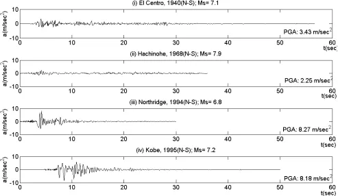
Four historic earthquake records are studied to assess the appropriateness of the

adaptive chirplet decomposition and the EMD to provide information about the

time-frequency characteristics of ground acceleration records pertaining to major earthquake

events. The El Centro (N-S component recorded at the Imperial Valley Irrigation District

substation in El Centro, California, during the Imperial Valley, California earthquake of

May 18, 1940), and the Hachinohe (N-S component recorded at Hachinohe City during

the Takochi-oki earthquake of May 16, 1968), earthquakes have been selected as far-field

examples. The Northridge (N-S component recorded at Sylmar County Hospital parking

lot in Sylmar, California, during the Northridge, California earthquake of January 17,

1994), and the Kobe (N-S component recorded at the Kobe Japanese Meteorological

earthquakes have been chosen as near-field examples [28,29]. Fig. (1) shows the

accelerograms of these strong ground motions.

The potential of the adaptive chirplet decomposition and the HHT for capturing

localized frequency content of nonlinear structural seismic responses is also examined.

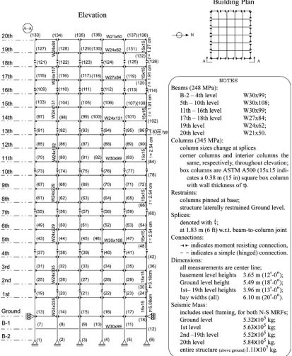
To this end, the nonlinear dynamic response of a benchmark 20-story steel frame [28,29]

to the above accelerograms is considered. It was designed by Brandow & Johnston

Associates for the SAC Phase II Steel Project and is part of a typical mid- to high-rise

building which meets the seismic code for the Los Angeles, California region.

The structural system consists of moment- resisting frames (MRFs), at the

perimeter to engage lateral loads, and simple framing in the interior. The columns are 345

MPa steel and the floors are composite with 248 MPa steel beams and concrete. The

model of the building along with information regarding various structural parameters is

shown in Fig. (2). The floors are assumed to be rigid in the horizontal plane and thus

diaphragmatic action holds. The inertia forces are assumed to be evenly distributed on the

two moment resistant frames. Symmetry allows an in-plane 2-D analysis of half of the

entire building and thus only one MRF along the weak N-S direction is considered. The

mathematic model described in Ohtori et al [28] is followed for the boundary conditions

and the discretization of the elastic and inertia properties of the frame. The first five

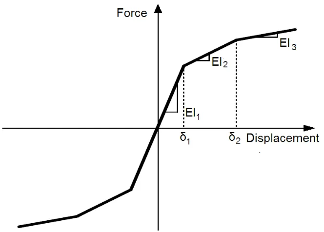
natural frequencies of the frame are 0.261, 0.753, 1.30, 1.83 and 2.40 Hz. A trilinear

hysteresis model for structural member bending, as the one shown in Fig. (3), is adopted.

More details on the trilinear model values considered for each member can be found in

5. Numerical results: Adaptive Chirplet Spectrograms and Hilbert Spectra

5.1 Seismic Accelerograms

Both the MP algorithm utilizing a Gaussian chirplet dictionary, and the EMD

algorithm have been employed to analyze the four accelerograms presented in Fig. (1).

Adequate representations of the earthquake signals were made possible by relatively

small numbers of terms: of order of fifty chirplet functions, and of less than ten intrinsic

modes, in all of the cases. Further, due to the adaptive nature of the decomposition

algorithms, the significant time-frequency characteristics of the earthquake signals were

captured by the very first few terms. Regarding the level of sophistication of the adaptive

chirplet decomposition, it is worth noting that the frequency modulation rate βk of the

chirplets hk was found to be negligible, as it has been reported before [23]. Thus, a

simpler dictionary of the three parametered Gabor atoms, instead of the four parametered

Gaussian chirplets, can be used yielding practically the same signal expansion. This

observation also suggests that the generation mechanisms of seismic events, the

propagation of seismic waves through the geological formations and the potential

influences of the surface soil layers do not produce signals whose complexity would

justify the use of Gaussian chirplets as analyzing functions.

Upon expanding the accelerograms into a series of chirplet functions, the WVD is

applied to yield the desired representation of these signals on the time-frequency plane.

Certain plots summarizing appropriate numerical results are provided in Figs. (4), (6), (8)

and (10), corresponding to the El Centro, Hachinohe, Northridge and Kobe earthquake

records, respectively. In the (a) plot of each figure the standard Fourier amplitude

chirplet spectrograms as computed by Eq. (17). In the (c) part of the aforementioned

figures contour plots of the adaptive spectrograms are presented to provide a more

efficient and practically useful joint time- frequency signal representation. The mean

instantaneous frequency (MIF) is superimposed, as obtained by the newly derived Eq.

(19), and the time histories of the accelerograms (d) are included, as well, to facilitate the

physical interpretation.

All surfaces shown in the (b) plots are exceptionally smooth throughout the

time-frequency plane and manifest the capacity of the Gaussian chirplets to represent the

signals considered with adequate resolution at all frequency bands of interest. By

comparing the corresponding (a) and (c) plots, it is obvious that the overall frequency

content provided by the Fourier amplitude spectra can equivalently be deduced by the

adaptive spectrograms. However, the latter capture, additionally, the evolution of the

frequencies present at every time instant of the records which illustrates the superiority of

a joint time-frequency analysis over the traditional Fourier analysis for earthquake

accelerograms. As expected, the higher frequencies prevail during the “growth phase” of

the accelerograms and then decay following a rate that is influenced by many parameters

whose consideration is beyond the scope of the present study.

In implementing the EMD, the basic algorithm and assumptions proposed by

Rilling et al [12], were adopted to balance precision versus computational cost, as it has

already been mentioned. The IMFs thus obtained yielded quite oscillating Hilbert spectra.

Low-pass filtering of the unwrapped phase of the IMFs and their associated amplitudes

by means of spline fitting was proved to be a necessity to achieve smoother results

spectra (Eq. (24)) and estimates of the MIF (Eq. (25)) based on the intrinsic mode

expansion are provided for the El Centro, Hachinohe, Northridge and Kobe earthquake

records, respectively.

As discussed earlier, the adaptive chirplet spectrogram enjoys a solid

mathematical background, which is not the case for the Hilbert spectrum based on the

IMFs. Evaluation of the performance of the EMD algorithm and of the smoothing

procedure of the IMFs is attempted by a qualitative comparison of the Hilbert spectra and

the MIF obtained by the IMFs with the corresponding adaptive spectrograms and the MIF

obtained by the Gaussian chirplets, for the four accelerograms considered. Specifically, it

can be seen from the figures provided, the two different types of time-frequency spectra

are consistent in the sense that the highest spectral values are attained at almost the same

time intervals and frequency levels. Furthermore, the trends of the temporal change of the

MIF exhibit a close similarity, even though the IMFs yield more oscillatory MIF

time-histories.

5.2 Structural response

Inelastic time-history dynamic analysis was performed for the 20- story steel

frame of Fig. (2) using as input the El Centro ground acceleration of Fig. (1) multiplied

by various factors. The standard β-Newmark algorithm with the assumption of constant

acceleration at each time step (values β=1/4, γ=1/2), was employed for the numerical

integration in time. In this manner, the non linear behavior of the frame stemming from

the adopted trilinear hysteresis model is properly taken into account, as described

The same decomposition algorithms used to analyze the seismic accelerograms

were next applied to the lateral displacement response signals of the first floor of the

frame under consideration as obtained by the above dynamic analysis. Herein, the

objective was to assess the potential of both methods for providing valid joint

time-frequency representations of non linear structural responses, for capturing the influence

of nonlinearity on the evolution of the effective natural frequencies of yielding structural

systems during a strong ground motion, and for demonstrating the effectiveness of the

MIF for global damage detection.

In the case of the adaptive chirplet expansion it has been observed that a

significantly smaller number of chirplets is required to fully describe the response signals

than in the case of the seismic accelerograms. This is due to the fact that structural

systems exhibit highly “resonant” transfer functions which filter the relatively broadband

earthquake signal inputs yielding response signals characterized by the structural natural

frequencies. Consequently, the MP algorithm readily locates the narrowband dominant

components present in the structural response signals by assigning appropriate weights to

the most similar analyzing functions to match efficiently these components. A Gabor

atoms dictionary yields practically the same decomposition of the structural response

signals as the one obtained by using Gaussian chirplets in the same way as it was noted in

the case of the analysis of the earthquake records.

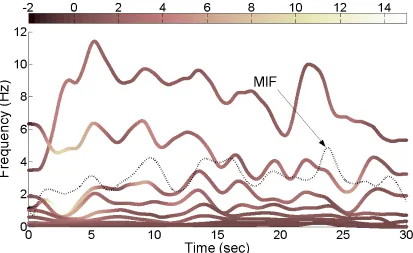
To demonstrate the potential of the MIF as analytical damage detection tool two

extreme cases are shown in Figs. (12) and (13) where the plots included are of the same

kind and order as in Fig. (10). In Fig. (12) the imposed excitation is the El Centro

Fig. (13) the El Centro accelerogram scaled by 2.50 is used as input and the frame suffers

structural damage witnessed by permanent deformation and a large offset component in

the Fourier spectrum. For reference purposes the first five natural frequencies of the

elastic frame are shown on the plots.

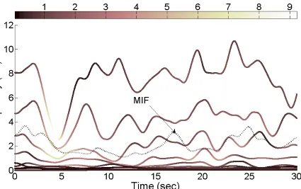
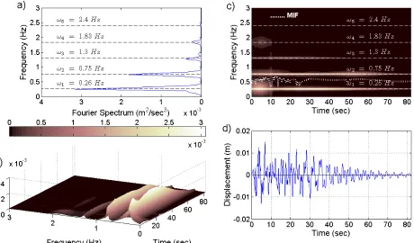
It is well known that structural systems forced to exhibit inelastic behavior are

characterized by gradually reduced effective natural frequencies, due to stiffness

degradation. Obviously, the variation in the “effective” natural frequencies of non linear

systems is reflected on the time-dependent transfer functions they attain and thus on the

output-response signals. In this context, the concentration of the energy of the response

signal about the natural frequencies of the frame which decrease when the frame

undergoes inelastic deformations can be readily seen in Figs. (12) and (13) in the

traditional Fourier spectrum plots (a), and in the adaptive spectrograms (b), (c).

Apparently, the joint time- frequency representation gives additional time localization

information about the effective frequencies of the response signals and adequately

captures their evolution in time.

More importantly, in this case the MIF can be interpreted as a global structural

damage indicator. The fundamental theorem of linear systems states that the spectrum of

the output signal is equal to the product of the Fourier transform of the input signal times

the transfer function of the system. Intuitively, for any particular effective temporal

segment defined such that the transfer function of the structure is assumed constant, the

MIF of the response averages this product over the frequency domain. Note that during

the first 25 seconds of both of the response signals examined in Figures (12c) and (13c)

MIF averages the product of the effective transfer function of the structure with the

spectrum of the excitation. Subsequently, the 30th second approximately marks the

effective duration of this particular input; practically the rest of the output signals

correspond to free vibration responses. As expected, after this time instant, the MIF

significantly decreases and remains in much lower levels for the scaled by 2.50 El Centro

input where the frame undergoes plastic deformations. However, in the elastic case, it

converges to a value similar to that attained at the beginning of the seismic event, since

the dynamic characteristics of the structure remain the same.

Prior to the application of the EMD, the response signals considered in this

analysis were limited to a bandwidth of approximately 0-5 Hz. The same algorithm was

applied as before and yielded again eight to ten IMFs for signal durations of 60 sec

sampled at the Nyquist frequency. Apparently, the number of the IMFs and the

computational cost of the EMD algorithm depend primarily on the length of the data and

not on the frequency content of the data which was the case for the MP algorithm and

adaptive chirplet decomposition, as was reported above.

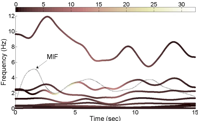
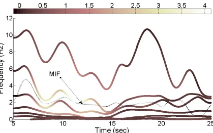
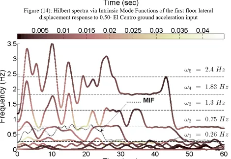
In Figs. (14) and (15), the Hilbert spectra of the decomposed lateral displacement

response of the first floor for the El Centro accelerogram input scaled by 0.50 and 2.50

are shown, respectively. The natural frequencies of the linear elastic system and the MIF

are also superimposed. The results show that the obtained IMFs are capable of capturing

the evolution of the natural frequencies of the structural system under consideration.

Nevertheless, the Hilbert spectra and the temporal variation of the MIF are not as smooth,

and amenable to physical interpretation compared to the corresponding adaptive

some IMFs are “attracted” by different natural frequencies during various time intervals.

This phenomenon can be reduced by introducing restrictions on the time interval between

successive extreme points attained by the IMFs based on the natural frequencies of the

analyzed system. Furthermore, additional low-pass filtering of the unwrapped phase and

amplitude of the IMFs can be used to yield less oscillating Hilbert spectra, at the expense

of poorer resolution. However, the later improvements require increased user/analyst

interaction in the form of parameter adjustments, rendering often the method less

appealing for practical purposes [27].

6. Concluding remarks

The present article has focused on the appropriateness, level of sophistication, and

comparative efficiency of certain adaptive signal analysis techniques for time-frequency

representation of non-stationary signals encountered in earthquake engineering problems.

In this regard, the adaptive chirplet transform (incorporating the MP algorithm), and the

EMD have been employed to analyze historic earthquake accelerograms and inelastic

structural response time histories to seismic signal inputs. Signals of this nature are

inherently non stationary as their intensity and frequency content varies with time and

thus require a joint time- frequency representation.

In this context, four ground acceleration records pertaining to two near-field and

two far- field major earthquake events have been decomposed into chirplet functions and

IMFs, and the WVD and Hilbert spectra of the decomposed signals have been obtained

respectively. A relatively small number of analyzing functions has been found to be

sufficient for the adequate approximation of the signals, while their main patterns and

found that a much simpler dictionary comprising Gabor atoms instead of Gaussian

chirplets yields an almost identical unfolding of the seismic signals in the time-frequency

domain and thus can be adopted to reduce the computational cost. The appropriateness of

the time-frequency representation to capture the evolving frequency content in time,

unlike the traditional Fourier amplitude spectrum, has been pointed out. Indeed, both

representations can be used as stand-alone time-frequency analysis tools. Note however

that despite the qualitative similarity of the two mathematically different representations,

the WVD is smoother and lends itself to easier physical interpretation compared to the

Hilbert spectrum.

Furthermore, both adaptive methods have been applied to the lateral displacement

response of the first floor of a 20-story steel frame exposed to one of the four

accelerograms scaled by appropriate factors to simulate undamaged and severely

damaged conditions for the structure. It has been found that significantly less chirplet

functions were sufficient to fully describe the response signals, than in the case of the

strong ground motion accelerograms, while the number of the required IMFs remained

practically the same, suggesting that the adaptive chirplet transform is much more

economical in terms of computational time. This observation can be attributed to the

highly resonant filtering effect of structural systems to broadband strong ground

excitations which facilitates the approximation of the response via chirp- type functions.

Furthermore, this concentration of the frequency content of the response signals about the

natural frequencies of the structure caused a characteristic mode-mixing in the IMFs

which obscures the physical interpretation of the Hilbert spectrum. This difficulty can be

during the EMD of the signal and by further smoothing the unwrapped phase and

amplitude of the resulting IMFs. Clearly, these measures require increased user/analyst

interaction in the form of parameter adjustments, and may render the adaptive chirplet

decomposition more attractive in practice vis-à-vis the EMD.

The potential of time-frequency representations of structural response signals as a

detection tool for global structural damage has been also pointed out. Specifically,

attention has been focused on the temporal evolution of the mean instantaneous

frequency. Indeed, if the structure is forced to exhibit inelastic behavior, the mean

instantaneous frequency reduces significantly reflecting the overall decrease of the

effective frequencies which is due to the structural stiffness degradation.

In conclusion, the findings of the present study show that both the adaptive

chirplet decomposition and the intrinsic modes decomposition are viable options for joint

time-frequency analyses of seismic signals. Furthermore, considering collectively these

two decompositions and the competing wavelet based decomposition, it is perhaps

premature to dispute any of the three as clearly the most advantageous for earthquake

engineering applications.

7. Acknowledgements

References

1. Cohen L. Time- Frequency Analysis. Upper Saddle River, NJ: Prentice-hall; 1995.

2. Burrus CS, Gopinath RA, Guo H. Introduction to wavelets and wavelet transforms- A

primer. Upper Saddle River, NJ: Prentice-hall; 1997.

3. Mallat S. A wavelet tour of signal processing. London: Academic Press; 1998.

4. Mann S, Haykin S. The chirplet transform: Physical considerations. IEEE Trans Signal

Process 1995;43(11):2745-2761.

5. Baraniuk RG, Jones DL. Wigner- based formulation of the chirplet transform. IEEE

Trans Signal Process 1996;44(12):3129-3135.

6. Huang NE, Shen Z, Long SR, Wu MC, Shih HH, Zheng Q, Yen NC, Tung CC, Liu

HH. The empirical mode decomposition and the Hilbert spectrum for nonlinear and

non-stationary time series analysis. Proc R Soc Lond A 1998;454:903-995.

7. Qian S. Introduction to time-frequency and wavelet transforms. Upper Saddle River,

NJ: Prentice-hall; 2001.

8. Chen SS, Donoho DL, Saunders MA. Atomic decomposition by basis pursuit. SIAM J.

Sci Comput 1998;20(1):33-61.

9. Mallat S, Zhang Z. Matching pursuits with time-frequency dictionaries. IEEE Trans

Signal Process 1993;41(12):3397-3415.

10. Qian S, Chen D. Signal representation via adaptive normalized Gaussian functions.

Signal Process 1994;36(1):1-11.

11. Yin Q, Qian S, Feng A. A fast refinement for adaptive gaussian chirplet

12. Rilling G, Flandrin P, Goncalves P. On empirical mode decomposition and its

algorithms. In: IEEE-EURASIP Workshop on nonlinear signal and image processing.

NSIP-03, GRADO(I); 2003.

13. Gabor D. Theory of communication. J. IEEE 1946;93(3):429-457.

14. Spanos PD, Failla G. Wavelets: Theoretical concepts and vibrations related

applications. Shock Vib Digest 2005;37(5):359-375.

15. Boashash B. Estimating and interpreting the instantaneous frequency of a signal. I.

Fundamentals. Proc IEEE 1992;80(4):520-538.

16. Flandrin P, Goncalves P. Empirical mode decompositions as data-driven wavelet-like

expansions. International Journal of Wavelets, Multiresolution & Information Processing,

2004;2(4):477-496.

17. Wang J, Fan L, Qian S, Zhou J. Simulations of non-stationary frequency content and

its importance to seismic assessment of structures. Earthquake Eng Struct Dyn

2002;31:993-1005.

18. Huang NE, Chern CC, Huang K, Salvino LW, Long SR, Fan KL. A new spectral

representation of earthquake data: Hilbert spectral analysis of station TCU129, Chi-Chi,

Taiwan, 21 September 1999. Bull Seism Soc Amer 2001;91(5):1310-1338.

19. Loh CH, Wu TC, Huang NE. Application of the empirical mode

decomposition-Hilbert spectrum method to identify near-fault ground-motion characteristics and

structural responses. Bull Seism Soc Amer 2001;91(5):1339-1357.

20. Zhang RR, Ma S, Hartzell S. Signatures of the seismic source in EMD-based

characterization of the 1994 Northridge, California, earthquake recordings. Bull Seism

21. Zhang RR, Ma S, Safak E, Hartzell S. Hilbert-Huang transform analysis of dynamic

and earthquake motion recordings. J. Eng Mech ASCE 2003;129(8):861-875.

22. Yang JN, Lei Y, Lin S, Huang N. Hilbert-Huang based approach for structural

damage detection. J. Eng Mech ASCE 2004;130(1):85-95.

23. Yan B, Miyamoto A. A comparative study of modal Parameter identification based

on wavelet and Hilbert-Huang transforms. Computer- aided civil and infrastructure

engineering. 2006;21(1):9-23.

24. Xu YL, Chen J. Structural damage detection using empirical mode decomposition:

Experimental investigation. J. Eng Mech ASCE 2004;130(11):1279-1288.

25. Zhang RR, Denmark LV, Liang J, Hu Y. On estimating site damping with soil

non-linearity from earthquake records. Int. J. Non-linear Mech. 2004;39:1501-1517.

26. Huang NE, Attoh-Okine NO, editors. The Hilbert-Huang transform in engineering.

Boca Raton, FL: CRC Press; 2005.

27. Kijewski-Correa T, Kareem A. Efficacy of Hilbert and wavelet transforms for

time-frequency analysis. J. Eng Mech ASCE 2006;132(10):1037-1049.

28. Ohtori Y, Christenson RE, Spencer BFJ, Dyke SJ. Benchmark structural control

problems for seismically excited nonlinear buildings. J. Eng Mech ASCE

2004;130(4):366-385.

29. Spencer BFJ, Christenson RE, Dyke SJ. Next generation benchmark control problems

for seismically excited buildings. In: Proceedings of the 2nd World Conference on

Structural Control. Kobori T et al. editors. Vol.2:1135–1360. Wiley, New York, 1999.

30. Roesset JM. Nonlinear dynamic response of frames. In: 8th Symposium on

31. Boashash B. Estimating and interpreting the instantaneous frequency of a signal. II.

Algorithms and applications. Proc IEEE 1992;80(4):540-568.

32. Olhede S, Walden AT. The Hilbert spectrum via wavelet projections. Proc R Soc

Figure (4): Joint time-frequency analysis of the El Centro accelerogram record via adaptive Gaussian chirplet expansion in conjunction with the Wigner-Ville distribution

Figure (6): Joint time-frequency analysis of the Hachinohe accelerogram record via adaptive Gaussian chirplet expansion in conjunction with the Wigner-Ville distribution

Figure (8): Joint time-frequency analysis of the Northridge accelerogram record via adaptive Gaussian chirplet expansion in conjunction with the Wigner-Ville distribution

Figure (10): Joint time-frequency analysis of the Kobe N-S accelerogram record via adaptive Gaussian chirplet expansion in conjunction with the Wigner-Ville distribution

Figure (12): Adaptive chirplet spectrogram of the first floor lateral displacement response to 0.50· El Centro ground acceleration input

Figure (14): Hilbert spectra via Intrinsic Mode Functionsof the first floor lateral displacement responseto 0.50· El Centro ground acceleration input