Exploring the relationship between population density and maternal health coverage

R E S E A R C H A R T I C L E

Open Access

Exploring the relationship between population

density and maternal health coverage

Michael Hanlon

, Roy Burstein

, Samuel H Masters

and Raymond Zhang

Abstract

Background:Delivering health services to dense populations is more practical than to dispersed populations, other factors constant. This engenders the hypothesis that population density positively affects coverage rates of health services. This hypothesis has been tested indirectly for some services at a local level, but not at a national level. Methods:We use cross-sectional data to conduct cross-country, OLS regressions at the national level to estimate the relationship between population density and maternal health coverage. We separately estimate the effect of two measures of density on three population-level coverage rates (6 tests in total). Our coverage indicators are the fraction of the maternal population completing four antenatal care visits and the utilization rates of both skilled birth attendants and in-facility delivery. The first density metric we use is the percentage of a population living in an urban area. The second metric, which we denote as a density score, is a relative ranking of countries by population density. The score’s calculation discounts a nation’s uninhabited territory under the assumption those areas are irrelevant to service delivery.

Results:We find significantly positive relationships between our maternal health indicators and density measures. On average, a one-unit increase in our density score is equivalent to a 0.2% increase in coverage rates.

Conclusions:Countries with dispersed populations face higher burdens to achieve multinational coverage targets such as the United Nations’Millennial Development Goals.

Keywords:Population density, Obstetric health coverage, Maternal and child health

Background

It has been recognized that some social services are more easily delivered to concentrated populations [1]. This argument has been implicitly applied to health ser-vices by two groups of researchers. The first group has used population density as an independent variable in analyses of coverage and outcomes. Studies of aggre-gated populations often incorporate population density as a continuous variable [2-4], while patient-level studies typically account for density as a binary, patient-level characteristic [5,6]. Generally, this literature includes population density as an afterthought, rather than a determinant of interest. A second group of researchers has estimated the effect of distance or travel time on service utilization [7-11]. This literature consistently

finds lower distances or travel times increase the utilization of some services. Yet travel times are a function of many factors, including how a population is distributed across space. Holding health system resources constant, a denser population is expected to face lower travel times than a dispersed population. So given the conclusions from the travel time literature, we hypothesize population density is an underlying de-terminant of some coverage rates.

An exhaustive test of this hypothesis would require data on coverage rates, population density, road networks and facility locations over time. To our knowledge, these data does not exist for any single country, let alone across countries. In this analysis, we conduct a cross-country, cross-sectional analysis of population density and coverage levels of three maternal health services. This is the first test of this relationship at a national level. We believe it is important because of the implica-tions for achieving multinational coverage targets such as * Correspondence:[email protected]

1

Institute for Health Metrics and Evaluation, University of Washington, 2301 5th Avenue, #600, Seattle, WA 98121, USA

Full list of author information is available at the end of the article

the United Nations’ Millennial Development Goals (MDGs) [12]. To the degree population density matters, countries with dispersed populations face higher burdens to achieve uniform targets like the MDGs.

Methods

We execute a cross-sectional analysis of 178 country-level observations. This is represented by equation (1),

in which the subscript c denotes a country-specific

variable. To hold the health system’s resources con-stant, we include per capita health expenditure and the number of hospital beds per 1,000 people in the coun-try. We further include the total fertility rate and the number of four-wheel vehicles per capita as determi-nants of demand. The hypothesis under consideration predicts β1> 0.

coveragec¼β0þβ1densityc

þβ2In health expenditureð Þ þβ3ðhospital bedscÞ

þβ4ðtotal fertility ratecÞ

þβ5ðfourwheel vehiclescÞ þεc ð1Þ

We use three different measures from 2009 as cover-age variables: (i) the percentage of pregnant women who complete four antenatal care visits prior to birth; (ii) the percentage use of a skilled birth attendant at delivery; and (iii) the percentage use of in-facility delivery ser-vices. These data series were produced by the Institute for Health Metrics and Evaluation (IHME) [13]. We chose IHME’s series because it is (to our knowledge) the most complete source of coverage estimates for these services at the national level. For health spending, we use the natural log of total per-capita health expenditure for 2009, as reported by the World Health Organization in real 2009 US dollars [14]. For the number of four-wheel vehicles, hospital beds and total fertility rate, we use data series from IHME [13]. These independent vari-ables are contemporaneous with the dependent variable because we expect little-to-no time lag in their effect on coverage levels.

A challenge with using population density is in identi-fying an appropriate metric to represent the concept. Prevailing density metrics may be inappropriate covari-ates in a cross-country analysis for a variety of reasons. For example, an unadjusted ratio of population-per-area at the national level includes uninhabited territory within a country’s borders. While those “empty spaces” may be relevant to some analyses, they are mostly irrele-vant to analyses of health service provision (service is not provided in areas without people). Therefore, the failure to discount uninhabited areas downwardly biases the population-per-area ratio in some countries. Metrics like the percentage of the population residing in an

“urban” or“dense”area are more appropriate to an ana-lysis of health service provision, but the definitions of

“urban” and “dense” can differ across countries [15,16]. There are attempts to reconcile these differences, but many approaches excessively conflate the relationship between density with wealth [17]. So it is unclear if pre-vailing metrics are appropriate for a cross-country com-parison, which may in part explain why so few analyses have considered population density’s effect on service provision [18].

To address this challenge, we separately use two mea-sures of population density: (i) percentage of the popula-tion residing in an “urban” area; and (ii) a novel metric designed for this analysis, which we denote as a coun-try’s “density score.” All these metrics are calculated using data from the Global Rural–urban Mapping Pro-ject (GRUMP) Alpha Version, from the year 2000 [19,20]. We choose to use GRUMP data for three rea-sons. First, we required a single dataset to provide popu-lation data at a global level. Second, in contrast to a dataset like LandScan, GRUMP is freely available to all users. Third, GRUMP provided extremely granular esti-mates in a consistently-measured scale. This is in con-trast to the Gridded Population of the World (GPW) dataset, which reported data at both higher and idiosyn-cratic levels of aggregation. For example, the GPW reports population and area by administrative unit, but the size of these units vary drastically across countries. In some countries vast tracts of unpopulated area were indistinguishable from population centers (Saudi Arabia’s territory was segmented into a mere thirteen units, most of which included both populous cities and large tracts of desert).

populations are assigned to uninhabited areas. This in-correct assignment is most likely to occur at the equa-tor because that is where grids are the largest. Yet even at the equator, grids are small enough (one square kilo-meter) that the magnitude of this problem is inherently limited. Also, metrics could be distorted if the grids were trivially small [22]. This is not a concern with this analysis because few consequential settlements exist above or below 65° latitude, let alone at the poles. This analysis is inherently global in perspective, and even for countries near the poles, the bulk of their population is measured in reasonably-sized grids of close to one square kilometer.

We employ GRUMP’s “unadjusted” population mates, which differ from published UN population esti-mates. An“adjusted”version of GRUMP exists in which population values are scaled so that country-level totals match published UN estimates. We use the unadjusted data, for two reasons. First, in percentage terms, the discrepancies were small. Second, the adjusted data was exposed to an additional transformation which was not relevant to this analysis. Moreover, it is unclear from the documentation precisely how that transformation was executed. The differences in estimates are not rele-vant to our findings, in that the“adjusted” metrics pro-duce the same results and lead to the same conclusions. Given the ambiguity of the adjustment process and its irrelevance to this analysis, we prefer the “unadjusted” metrics.

GRUMP identifies “urban” grids in the dataset. We use the population values assigned to those grids to cal-culate our first density metric, which is the percentage of the country’s total population residing in an urban area. However, GRUMP uses satellite imagery of night-lights to identify urban areas, which is potentially prob-lematic because nightlight usage has been shown to be strongly influenced by wealth [23,24]. This is an issue for this analysis because we attempt to identify density’s effect independently of wealth. So while this metric is generally accepted, it is uncleara priorihow appropriate its usage is in this analysis. This concern leads us to gen-erate country-level density scores.

To calculate a density score, we first use the GRUMP data to determine global density decile thresholds, such that each density decile contains 10% of the global population. Then for each country, we determine the percentage of the population residing in each global de-cile. In other words, we sum the population of each grid in a country assigned to each global decile, and then divide by the country’s total population. This is represented by equation (2), in which d and popc,d de-note the decile and the corresponding percentage of the population from country c in that decile. For each country, we calculate a weighted average in which the

weights increase along with the decile, per equation (3). This weighted average is a country’s density score.

popc;d¼

population residing in grids with density belonging to deciled

total population of countryc ð2Þ

scorec¼

X10

d1 d1

9 ∗popc;d

∗100 ð3Þ

Our method to calculate a density score is conceptu-ally similar to the procedure outlined by Craig (1984), who examined population density data in Great Britain [25]. Given these scores are based on global density dec-iles, it is effectively a relative ranking of density across countries. If a country’s entire population resides in the lowest global decile, its score is zero. If the entire popu-lation resides in the highest decile, its score is one hun-dred. If a country’s density mirrors the global density, such that one-tenth of its population resides in each de-cile, its score is fifty. We could have adopted a different quantile to generate the scores, such as using vigintiles or percentiles rather than deciles. Also, we could have adopted a different weighting scale, rather than the uni-form discounting in equation (3). An infinite number of options exist, many of which would have a marginal im-pact on the distribution (although not the order) of the scores. Given our regression model is most sensitive to the order, this choice has limited impact on this study. However, it could impact the magnitude of the effect, and therefore any policy implications (see the Discussion section).

Results

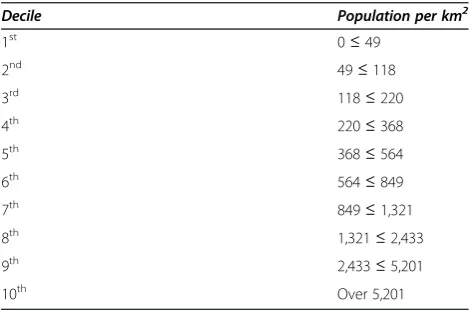
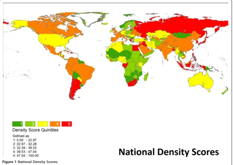
Table 1 reports thresholds for global population density deciles for the year 2000, as calculated from GRUMP data. From this data, 50% of the global population resided in an area with a population density exceeding 564 persons per square kilometer. Figure 1 is national-level map of density scores by quintile. Several countries

Table 1 Global population density deciles

Decile Population per km2

1st 0≤49

2nd 49≤118

3rd 118≤220

4th 220≤368

5th 368≤564

6th 564≤849

7th 849≤1,321

8th 1,321≤2,433

9th 2,433≤5,201

highlight how consequential our weighting process is to the results. Via an unadjusted calculation of population per area, Russia’s density is less than 10 persons per square kilometer and Egypt’s density is approximately 30 persons per square kilometer. By that metric, popula-tions in both countries seem extremely dispersed. Yet once uninhabited areas are discounted, both countries emerge as being very dense because their populations are condensed in relatively small areas.

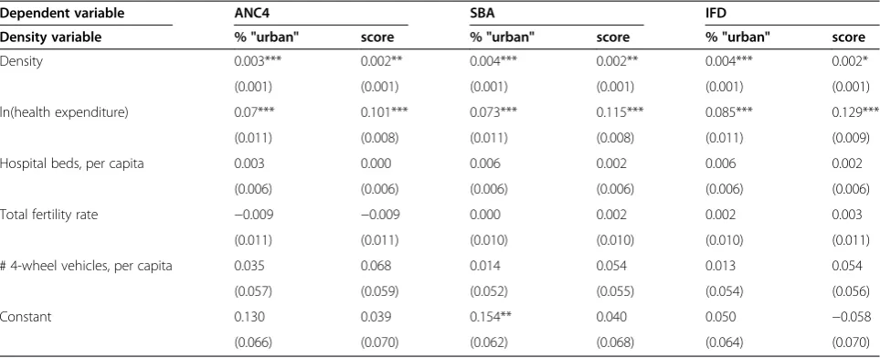
Table 2 reports descriptive statistics of the variables used in the regression analysis (the webappendix reports all the data used in this analysis at the country level). Re-gression results with robust standard errors are pub-lished in Table 3. Across the six regressions, a total of 10 observations were clearly outliers but the results are robust to their exclusion. When comparing our two density metrics, we find the “percentage urban” variable consistently has a larger (and thus more significant)

Figure 1National Density Scores.

Table 2 Descriptive statistics

Variable Mean Standard deviation Median Skewness

Antenatal visits (rate completing four) 0.693 0.218 0.787 −0.93

Skilled birth attendant (rate) 0.819 0.232 0.958 −1.28

In-facility delivery (rate) 0.793 0.249 0.941 −1.13

Percent population "urban" 52.8 24.6 55.2 −0.08

Density score 35.9 13.9 34.8 0.52

Log per capita health expenditure 6.0 1.4 6.1 0.00

Hospital beds, per 1000 population 3.7 3.0 2.7 0.97

Total fertility rate 2.9 1.5 2.4 0.90

effect on coverage rates than the density score. However, when using the“percentage urban”as a predictor, the ef-fect of health spending decreases. This may be due to the conflation of population density and wealth dis-cussed in the Methods section. This concern is sup-ported by the correlations in the density variables with health expenditure: it equals 0.73 for “percent urban” but decreases to 0.30 for the density score. This leads us to prefer the density score as the appropriate metric to represent density in this analysis.

Across the three regressions which use the density score, the effects of per-capita expenditure and the dens-ity scores were significantly positive. The model has an untransformed dependent variable, but expenditure is included as a natural log. So the interpretation is that an increase of e (2.7182. . .) in expenditure would produce an increase of β in coverage. Point estimates ranged from 0.101 for antenatal visits to 0.129 to in-facility de-livery. Therefore, on average, an increase in health ex-penditure per capita of 2.71 times is associated with a 12.9% increase in the use of in-facility delivery services. Regarding the density score, a one unit increase in a country’s score translates to a 0.2% increase in coverage for all three considered in this analysis. The number of hospital beds, the fertility rate and the number of vehi-cles failed to achieve statistical significance.

Discussion

Increasing the log of health expenditure per capita by one unit had the effect of increasing coverage roughly 11% across the three interventions. This implies that in-creasing health expenditure per capita by 1% has the ef-fect of increasing coverage by roughly 0.04%. In contrast, increasing the population density score by a

single unit had the effect of increasing coverage by 0.2%. This comparison highlights that population density mat-ters, but national policy makers’ability to manage dens-ity is constrained. So as a practical matter, health expenditure is a more important determinant of interest. Yet these results suggest different countries face differ-ent challenges in realizing multinational targets like the MDGs. For example, Benin and Mali have similar per capita expenditure on health. However, Benin’s popula-tion is far denser than Mali’s, and Benin’s coverage rates are considerably higher. Population density may in part explain that difference.

Density scores could be valuable to some policy makers if they were calculated at a regional or national level, rather than a global level. For example, analysts fo-cused on African societies could develop scores derived from African density deciles, or US states could be assigned density scores based on US population deciles. While policy makers do not control population density per se, they do control factors which are likely to affect it, such as road construction or building codes in devel-oped countries. Ultimately, the appropriate choice is a function of the specific analysis under consideration. Yet we believe the approach described in this analysis is a methodological improvement over the use of prevailing measures of population density, and thus merits consid-eration from analysts interested in controlling for popu-lation density.

As noted in the Methods section, the magnitude (al-though not the direction) of the reported results could be contingent on the method used to calculate the scores. Consider a weighting scale which discounted dif-ferences between the lowest deciles and exaggerated them between the higher deciles. For clarity, a priori

Table 3 Regression results

Dependent variable ANC4 SBA IFD

Density variable % "urban" score % "urban" score % "urban" score

Density 0.003*** 0.002** 0.004*** 0.002** 0.004*** 0.002*

(0.001) (0.001) (0.001) (0.001) (0.001) (0.001)

ln(health expenditure) 0.07*** 0.101*** 0.073*** 0.115*** 0.085*** 0.129***

(0.011) (0.008) (0.011) (0.008) (0.011) (0.009)

Hospital beds, per capita 0.003 0.000 0.006 0.002 0.006 0.002

(0.006) (0.006) (0.006) (0.006) (0.006) (0.006)

Total fertility rate ₋0.009 ₋0.009 0.000 0.002 0.002 0.003

(0.011) (0.011) (0.010) (0.010) (0.010) (0.011)

# 4-wheel vehicles, per capita 0.035 0.068 0.014 0.054 0.013 0.054

(0.057) (0.059) (0.052) (0.055) (0.054) (0.056)

Constant 0.130 0.039 0.154** 0.040 0.050 −0.058

(0.066) (0.070) (0.062) (0.068) (0.064) (0.070)

there is no sensible reason to adopt this strategy versus the one we employed. However, if an analyst’s objective was to exaggerate differences among the higher deciles, then an appropriate strategy might be to use the quad-ratic weight (d-1/9)2 rather than d-1/9. This would skew

the distribution of scores leftward (similarly, the square root of d-1/9 would exaggerate the difference between

the lowest deciles and skew the distribution rightward). Depending on the intervention under consideration, this skewness could impact (any likely impair) any statistical inference. It is important to note that skewness could lead to heteroskedasticity, and thus inefficient estimation [26]. In some cases, this could prevent an analyst from identifying an effect which exists in reality. Yet this ex-ample is not intended to suggest score distributions must necessarily be symmetric, or that exaggerating the difference between the lowest or highest deciles is uni-versally inappropriate. Rather, the key point is that the metric’s construction might be relevant to some ana-lyses, and analysts should consider those complexities when replicating our strategy to measure population density.

Conclusion

This analysis examines how population density influ-ences maternal health coverage. This is the first attempt to identify this relationship at a national level. We find that population density positively influences coverage, and the implications of this conclusion are significant for demographers, public health researchers and policy makers. Countries with low population densities face higher burdens to achieve coverage of some health ser-vices. Therefore, we predict those countries require more resources per capita to achieve multinational coverage targets such as the MDGs.

Competing interests

The authors have no competing interests to declare.

Authors_’contributions

MH devised the analytical strategy, including the notion of density scores, and authored the draft. RB processed geospatial data from GRUMP. SHM and RZ conducted the empirical analysis. All authors read and approved the final manuscript.

Acknowledgements

We owe thanks to Kelsey Moore for her project management. This research was supported by the Institute for Health Metrics and Evaluation’s core funding from the Bill & Melinda Gates Foundation.

Author details 1

Institute for Health Metrics and Evaluation, University of Washington, 2301 5th Avenue, #600, Seattle, WA 98121, USA.2_{Feinberg School of Medicine,}

Northwestern University, Seattle, USA.

Received: 8 June 2012 Accepted: 15 October 2012 Published: 21 November 2012

References

1. Rank MR, Hirschl TA:The link between population density and welfare participation.Demography1993,30(4):607–622.

2. Newacheck PW, Hung Yun Y, Park MJ, Brindis M, Irwin CE:Disparities in adolescent health and health care: does socioeconomic status matter? Health Serv Res2003,38(5):1235_–1252.

3. Wright JA, Polack C:Understanding variation in measles-mumps-rubella immunization coverage—a population-based study.Eur J Public Health 2005,16(2):137_–142.

4. Mitchell R, Popham F:Effect of exposure to natural environment on health inequalities: an observational population study.Lancet2008, 372(9650):1655–1660.

5. Terschuren C, Mensing M, Mekel OCL:Is telemonitoring an option against shortage of physicians in rural regions? Attitude towards telemedical devices in the North Rhine-Westphalian health survey, Germany.BMC Health Serv Res2012,12(95). doi:10.1186/1472-6963-12-95.

6. Lu,et al:Outcomes of prolonged mechanic ventilation: a discrimination model based on longitudinal health insurance and death certificate data.BMC Health Serv Res2012,12(100). doi:10.1186/1472-6963-12-100. 7. Lovett A, Haynes R, Sünnenbergand G, Gale S:Car travel time and

accessibility by bus to general practitioner services: a study using patient registers and GIS.Soc Sci Med2002,55.1:97_–111.

8. Tanser F, Gijsbertsen B, Herbst K:Modelling and understanding primary health care accessibility and utilization in rural South Africa: an exploration using a geographical information system.Soc Sci Med2006, 63.3:691–705.

9. Astell-Burt T, Flowerdew R, Boyle PJ, Dillon JF:Does geographic access to primary healthcare influence the detection of hepatitis C?Soc Sci Med 2011,72.9:1,472–1,481.

10. Alegana VA, Wright JA, Pentrina U, Noor AM, Snow RW, Atkinson PM: Spatial modeling of healthcare utilization for treatment of fever in Namibia.Int J Health Geogr2012,11:6.

11. Gabrysch S, Cousens S, Cox J, Campbell OM:The influence of distance and level of care on delivery place in rural Zambia: a study of linked national data in a geographic information system.PLoS Med2011,8.1:e1000394. doi:10.1371/journal.pmed.1000394.

12. United Nations:Millennium Development Goals Report 2011; June 2011, ISBN 978-92-1-101244-6, available at: http://www.unhcr.org/refworld/docid/ 4e42118b2.html [accessed 5 June 2012].

13. Institute for Health Metrics and Evaluation:Health Metrics Covariate Database. Seattle, WA: Institute for Health Metrics and Evaluation; 2011. 14. World Health Organization:National Health Accounts: Country Health

Information; Source (accessed April 2011): http://www.who.int/nha/ country/en/.

15. United Nations Statistical Division; Source (accessed October 2011): http:// unstats.un.org/unsd/demographic/sconcerns/densurb/densurbmethods.htm. 16. Haggblade S, Longabaugh S, Tschirley DL:Spatial patterns of food staple

production and marketing in South East Africa: implications for trade policy and emergency response.Unpublished manuscript: http:// econpapers.repec.org/paper/agsmidiwp/54553.htm.

17. Nations U:World Urbanization Prospects: The 2009 Revision. New York, NY: The United Nations; 2009.

18. Galea S, Freudenberg N, Vlahov D:Cities and population health.Soc Sci Med2005,60(5):1017–1033.

19. Center for International Earth Science Information Network, Columbia University; International Food Policy Research Institute; The World Bank; and Centro Internacional de Agricultura Tropical:Global Rural–urban Mapping Project (GRUMP), Alpha Version. Palisades: Socioeconomic Data and Applications Center, Columbia University; 2004. Data downloaded November 2010 from http://sedac.ciesin.columbia.edu/gpw.

20. Balk D:More Than a Name: Why Is Global Urban Population Mapping a GRUMPy Proposition?InGlobal Mapping Of Human Settlements: Experiences, Datasets and Prospects. Edited by Gamba P, Herold M. Boca Raton: CRC Press; 2009.

21. Haaland CM, Health MT:Mapping of Population Density.Demography 1974,11(2):321–336.

22. Stairs RA:The concept of population density: a suggestion.Demography 1977,14(2):243_–244.

24. Elvidge CD, Baugh KE, Kihn EA, Kroehl HW, Davis ER, Davis CW:Relation between satellite observed visible-near infrared emissions, population, economic activity and electric power consumption.Int J Remote Sensing 2010,18(6):1373–1379.

25. Craig J:Averaging population density.Demography1984,21(3):405–412. 26. Cameron CA, Trivedi PK:Microeconometrics: Methods and Applications.

Cambridge, UK: Cambridge University Press; 2005.

doi:10.1186/1472-6963-12-416

Cite this article as:Hanlonet al.:Exploring the relationship between

population density and maternal health coverage.BMC Health Services

Research201212:416.

Submit your next manuscript to BioMed Central and take full advantage of:

• Convenient online submission

• Thorough peer review

• No space constraints or color figure charges

• Immediate publication on acceptance

• Inclusion in PubMed, CAS, Scopus and Google Scholar

• Research which is freely available for redistribution