karya ini dan pada pandangan saya / kami karya ini
adalah memadai dari segi skop dan kualiti untuk tujuan penganugerahan
Ijazah Sarjana Muda Kejuruteraan Mekanikal (Design&Inovasi)
Tandatangan
:
Nama penyelia I
:
Tarikh
:
Tandatangan
:
Nama penyelia II
:
NURUL HAFIDZAH BINTI ROSLI
Laporan ini dikemukakan sebagai memenuhi syarat sebahagian daripada syarat
penganugerahan Ijazah Sarjana Muda Kejuruteraan Mekanikal (Design&Inovasi)
Fakulti Kejuruteraan Mekanikal
Universiti Teknikal Malaysia Melaka
“Saya akui laporan ini adalah hasil kerja saya sendiri kecuali ringkasan dan petikan yang
tiap-tiap satunya saya telah jelaskan sumbernya”
Tandatangan
:
Nama Penulis
:
ACKNOWLEDGEMENT
Greatest thanks to Allah Almighty for His blessings and giving me the
ability to finish this project, which hopefully can contribute in further research.
I would like to express my gratitude and appreciation to my respectful
lecturer supervisor, Mrs. Zakiah bt. Abd Halim for her supervision, invaluable
advice and inspiring encouragement in guiding me in completing this research.
Further acknowledgements also to all lecturers and technicians at Faculty
of Mechanical Engineering at UTeM for their technical support and help during
the completion of this work. Especially to Mr. Rizal from NDT Lab who help
sincerely throughout Ultrasonic Testing experiment. Not forgotten to Mr. Sahar
and all staff in Advanced Manufacturing Centre that help in manufacturing
process even though in their hectic schedule.
Last but not least, I would like to express my gratitude and affection to
my beloved family and friends for their unconditional support and smile during
developing the original version of this style document.
ABSTRACT
ABSTRAK
Kajian ini khusus untuk mengkaji kesan frekuensi pemindaharuh
ultrabunyi yang berbeza di dalam penggunaan pemeriksaan ultrabunyi. Dari
kajian literatur, kajian mengenai kesan penggunaan frekuensi pemindaharuh
ultrabunyi yang berbeza masih tidak jelas lagi dibincangkan sehingga ke hari
ini. Pemeriksaan ultrabunyi merupakan cabang Kajian Tanpa Musnah yang
digunakan secara meluas untuk mengesan kecacatan serta menguji kedalaman
spesimen tanpa memusnahkannya.
Dalam bab metodologi, bahan ujikaji telah
direka dan difabrikasi menggunakan mesin CNC Universal Milling Machine for
5-Axis. Untuk eksperimen ini, jenis pemindaharuh bunyi satu kristal akan
digunakan dengan pemindaharuh bunyi frekuensi sebagai pembolehubah yang
dimanipulasikan di mana 2 MHz, 4 MHz dan 5 MHz digunakan. Hasil
eksperimen ini ialah pantulan tenaga suara dari ‘A-scanned’. Dari pemerhatian,
pemindaharuh berfrekuensi tinggi mempunyai amplitud yang rendah, kurang
gangguan bunyi dan puncak yang tajam sementara pemindaharuh berfrekuensi
rendah menunjukkan amplitud yang tinggi, gangguan bunyi yang tinggi dan
puncak yang lebar.
Melalui keputusan ini, perbezaan ciri untuk setiap peringkat
frekuensi di mana tinggi (5 MHz) dan rendah (2MHz) dibincangkan.
Ciri-ciri
TABLE OF CONTENT
CHAPTER
INDEX
PAGE
ACKNOWLEDGEMENTS
і
ABSTRACT
іі
ABSTRAK
ііі
TABLE OF CONTENT
v
LIST OF TABLE
vііі
LIST OF FIGURE
x
LIST OF APPENDIX
v
CHAPTER 1
INTRODUCTION
1
1.1
Background of project
2
1.2
Problem statement
3
1.3
Objective
3
1.4
Scope
3
CHAPTER 2
LITERATURE REVIEW
4
2.1
An overview of Ultrasonic
4
2.1.1 Piezo-electric Effect
5
2.1.2 Ultrasonic Processors
6
2.1.3 Ultrasonic Probes
7
CHAPTER
INDEX
PAGE
2.2
Previous research
9
CHAPTER 3
METHODOLOGY
14
3.1
Introduction
14
3.2
Material
15
3.3
Research design
16
3.4
Design Analysis
17
3.5
Fabrication of Test Sample
19
3.6
Ultrasonic Testing
20
3.6.1 Equipments
21
3.6.2 Procedure
22
3.6.3 Parameter of Study
23
3.6.3.1 Objective: To investigate
effect of probe frequency
23
3.6.3.2 Objective: To investigate
the effect of test sample
material for probe
frequency selection
24
CHAPTER 4
RESULT
25
4.1
Effect of Probe Frequency
25
4.2
Effect of Test Sample Material for Probe
Frequency Selection
39
4.3
Crack Location
43
CHAPTER 5
DISCUSSION
44
5.1
Introduction
44
CHAPTER
INDEX
PAGE
5.3
Effect of Test Sample Material for Probe
Frequency Selection
47
5.4
Design Factor
49
5.5
Error Analysis
52
CHAPTER 6
CONCLUSION AND RECOMMENDATION
61
6.1
Conclusion
61
6.2
Recommendation
62
REFERENCES
63
BIBLIOGRAPHY
66
LIST OF TABLE
NUMBER TITLE
PAGE
3.1
Material Properties for Mild Steel
15
3.2
Material Properties for Aluminum
15
3.3
To Study Effect of Probe Frequency
23
3.4
To Study the Effect of Test Sample Material for Probe
Frequency Selection
24
4.1
Result of Backwall for Different Probe Frequency
27
4.2
Result of Crack 1 at Position A to B for Different Probe
Frequency
30
4.3
Result of Crack 1 at Position B to C for Different Probe
Frequency
31
4.4
Result of Crack 1 at Position C to D for Different Probe
Frequency
33
4.5
Result of Crack 3 at Position A to B for Different Probe
Frequency
NUMBER TITLE
PAGE
4.6
Result of Crack 1 at Position C to D for Different Probe
Frequency
38
4.7
Result of Backwall for Mild Steel and Aluminum
40
4.8
Result of Crack 1 at Position A to B for Mild Steel and
Aluminum
41
4.9
Result of Crack 1 at Position A to B for Mild Steel and
Aluminum
42
4.10
Result of Crack 6 for Mild Steel and Aluminum
43
5.1
Relative Error for Effect of Probe Frequency Experiment
53
5.2
Relative Error Calculation for Effect of Test Sample
Material for Probe Frequency Selection Experiment
56
5.3
Thickness Analysis of Mild Steel
58
5.4
Thickness Analysis of Aluminum
59
LIST OF FIGURE
NUMBER TITLE
PAGE
2.1
Acoustic Spectrum [1]
5
2.2
Ultrasonic Processor [4]
6
3.1
Overview of Research Methodology
14
3.2
Flow Process for Research Design
16
3.3
Final Test Sample Drafting and Cross Section
17
3.4
Layered Crack
18
3.5
CNC 5-Axis Face Milling (DMG-DMU250) [22]
19
3.6
Milling Machining Process[23]
20
3.7
Equipment for Ultrasonic Testing
21
3.8
IOW Calibration Block
22
4.1
2 MHz Result for Backwall
26
4.2
4 MHz Result for Backwall
26
4.3
5 MHz Result for Backwall
27
4.4
Crack 1 Cross Section
27
4.5
2 MHz Result for Crack 1 at Position A to B
28
4.6
4 MHz Result for Crack 1 at Position A to B
29
4.7
5 MHz Result for Crack 1 at Position A to B
29
4.8
2 MHz Result for Crack 1 at Position B to C
30
4.9
4 MHz Result for Crack 1 at Position B to C
30
4.10
5 MHz Result for Crack 1 at Position B to C
31
4.11
2 MHz Result for Crack 1 at Position C to D
32
4.12
4 MHz Result for Crack 1 at Position C to D
32
4.13
5 MHz Result for Crack 1 at Position C to D
33
4.14
5 MHz Result for Crack 2 at Position B to C
34
4.15
Cross Section of Crack 3
34
4.17
4 MHz Result for Crack 3
35
4.18
5 MHz Result for Crack 3
36
4.19
Cross Section for Crack 6
37
4.20
2 MHz Result for Crack 6
37
4.21
4 MHz Result for Crack 6
37
4.22
5 MHz Result for Crack 6
38
4.23
4 MHz Result for Aluminum Backwall
40
4.24
4 MHz Result for Aluminum for Crack 1 at Position A
to B
40
4.25
4 MHz A-Scan Result for Aluminum at Crack 3
41
4.26
4 MHz A-Scan Result for Aluminum at Crack 6
42
4.27
Crack Location and Shape
43
5.1
Graph Gain & Pulse Delay Versus Frequency for
Backwall
45
5.2
A-Scan Backwall for 2 MHz and 5 MHz
45
5.3
Graph Gain & Pulse Delay Versus Frequency for Crack
1 at Position A to B.
47
5.5
A-Scan Back Wall for Mild Steel and Aluminum
48
5.6
A-Scan Crack 1 at Position A to B for Mild Steel and
Aluminum
49
5.7
A-Scan Crack 2 at Position B to C for 2 MHz and 5
MHz
50
5.8
A-Scan at Crack 3 for 2 MHz and 5 MHz
50
LIST OF APPENDIX
NUMBER TITLE
PAGE
1A
GANTT CHART
67
3A
Test Sample Design
70
3B
Final Test Sample Design
72
3C
Crack Cross Section
73
3D
The CNC 5-Axis Face Milling Technical Specification
74
3E
Test Sample CATprocess File
75
3F
Programming
76
3G
Machining Process
107
4A
A-Scan Result Effect of Probe Frequency Experiment
108
4B
A-Scan Result for 4 MHz Aluminum
115
CHAPTER 1
INTRODUCTION
1.1
Background of the project
1.2
Problem Statement
Transducer or probe is one of the basic component for an ultrasonic testing
system. It is manufactured in variety of forms, shapes and sizes to suit for varying
applications. Selection of correct probe frequency is one of the critical parameter to
optimize the Ultrasonic Testing capabilities. Proper selection is important to ensure
accurate inspection data as desired for specific applications. Therefore, an investigation
is required to specify the suitability of different range of probe frequency.
1.3
Objective
This project is conducted to investigate the effect of selection of probe frequency
in Ultrasonic Testing results and specify the suitability of different range of probe
frequency in Ultrasonic Testing. In this project, the test sample for the experiment will
be design and the suitability of probe frequency in Ultrasonic Testing will be
investigated experimentally.
1.4
Scope
CHAPTER 2
LITERATURE REVIEW
2.1
An overview of Ultrasonic
Since the publication of Lord Rayleigh’s work on sound in “The Theory of
Sound”; this work explained the nature and properties of sounds waves which led to the
development of the techniques that are currently in use in nondestructive testing [2].
Ultrasounds or Ultrasonics is a sound that generated above the human hearing
range. Vibrations above 20 KHz are termed “Ultrasonic waves”. 0.5 MHz to 20 MHz is
the usual frequency range for ultrasonic flaw detection[2,3]. However, from [1], the
frequency range for ultrasonic nondestructive testing and thickness gage is 0.1 MHz to
50 MHz. The Piezo-Electric Effect is used to produce these high frequencies [2,4,5].
Although ultrasound behaves in a similar manner to audible sound, it has a much shorter
wavelength. This means it can be reflected off very small surfaces such as defects inside
materials. It is this property that makes ultrasound useful for nondestructive testing of
materials.
Figure 2.1: Acoustic Spectrum [1]
From the figure above, the part of the spectrum from zero to 16 Hz is below the
range of human hearing and is called the ‘Subsonic’, or ‘Infrasonic’ range. From 16 Hz
to 20 KHz is known as the ‘Audible’ range and above 20 KHz as the ‘Ultrasonic’ range.
Ultrasonic flaw detection uses vibrations at frequencies above 20 KHz.
Most flaw detection takes place between 500 KHz and 20 MHz although there
are some applications, for example in concrete, that use much lower frequencies and
there are special applications at frequencies above 20 MHz. In most practical
applications in steels and light alloys, frequencies between 2 MHz and 10 MHz
predominate. Generally the higher the test frequency, the smaller the minimum
detectable flaw, but it will be shown in following articles that higher frequencies are
more readily attenuated by the test structure. Choosing an appropriate test frequency
becomes a compromise between the size of flaw that can be detected and the ability to
get sufficient sound energy to the prospective flaw depth [3].
2.1.1 Piezo-electric Effect
energy to mechanical energy or vice-versa are called transducer which are incorporated
in device call probe. Usually this probe manufactured from a number of materials such
as quartz and ceramic. The vibrating crystal is used to produce ultrasonic compression
waves within the probe [3].
2.1.2 Ultrasonic Processors
Ultrasonic processors consists of three major components; power supply
(generator), a converter (transducer) and a probe (horn)[4].
Figure 2.2: Ultrasonic Processor [4]
From the Figure 2.2, power supply generates energy from the electrical power.
Then this electrical energy is convert to mechanical energy using transducer. To increase
amplitude, booster is used. Lastly, probe increases the amplitude and transfer the
vibrations to the tested blocks.
5
0
/6
0
Hz
Elect
rical
po
we
r
2
0
kHz
Elect
rical
e
n
erg
y
2
0
kHz
Vi
b
ratio
n
s
2
0
kHz
Vi
b
ratio
n
s
2
0
kHz
Vi
b
ratio
n
However, according to Heiller C.J. others termed to describe the transducer are
“probe”, “search unit”, and “test head” [2]. Throughout this research transducer will
refer as probe.
2.1.3 Ultrasonic Probes
Probes are also one-half-wavelength-long section that act as mechanical
transformers to increase the amplitude of vibration generated by the converter. Probes
are made to resonate at a specific frequency. 20 kHz probes are typically 5 inch and can
be made longer in 5 inch increments. 40 kHz probes are typically 2.5 inch long and can
be made longer in 2.5 inch increments [4].
2.1.4 Frequency
For frequency selection between varied instruments by respective manufactures
it is important to predetermined nominal frequency of the transducer operated based on
their thickness. Though the probe oscillates at its resonant frequencies, but other
frequency produce, some higher and some lower than the nominal center frequency.
Some undesirable frequencies are filtered out because they produce low-level noise and
by this can reduce “the signal-to-noise” ratio. The signal from a reflector must be visible
above the background noise caused by material grain and other factor such as instrument
circuit noise [2].
narrow band receivers is usually user-selectable. In this case, the user the user selects the
frequency nearest to that of the transducer being used. The effect is that receiver
processes only the frequency selected, within a certain “bandwidth”. This circuitry will
filter out frequencies outside this bandwidth. Another name for this type is “bandpass
filter”. There are other types of filters. Those that allow frequencies higher than a certain
value to be processed are called “low-pass filters”. When conducting a test on very
grainy material, low-frequency energy is used to help overcome the grain noise. In this
case, it is advantageous to use a low-pass filter to reject the scattered higher-frequency
energy. This usually helps to increase the signal-to-noise ratio and provide superior data
[2].
The frequencies of the probe element determines the wavelength of the
ultrasound within the test material. Combined with the geometry of the element, the
frequency also establishes the exent of the near-field or natural focusing point and the
amount of beam-spreading in the far-field or the points beyond the focal point [6].
The higher the frequency the greater the attenuation by absorption and scatter,
therefore, when working on coarse grain structures which cause high attenuation a lower
frequency probe is selected. Attenuation is the decreasion of sound pressure when a
wave travels through a material arising from absorption and scattering.
Lowering the frequency has the effect of increasing the beam angle. To
overcome this we can increase the crystal diameter.
A probe with good resolution will be able to detect small defects and will be able
to resolve defects which are close together [3].
The environment factors should be concern when using Ultrasonic Testing
devices. The factors consist of temperature, air turbulence and convection currents,
atmospheric pressure, humidity, acoustic interference, radio frequency interference and
splashing liquids. The other possible factor that will affecting Ultrasonic Testing
experiment are composition, shape, target orientation to sensor and averaging [7].
2.2
Previous research
A studies of Automation of Ultrasonic Testing Procedures has been conducted. It
involves the use of both longitudal and transverse high-frequency sound waves for the
exploration and/or mapping of both surface and sub-surface defect or irregularaties. The
aim for this studies is to determine the location of defects, the size of defects and
acceptability of the defects in the specimen. However this research is only focusing on
the procedure, so there are no discussion of the A-scan readings and potentials errors.
USD 15 ultrasonic flaw detector and 90° probe is used. The frequency that suggested is
0.5 MHz to 20 MHz [8].
According to the research of Ultrasonic detection of defects in strongly
attenuating structures using the Hilbert–Huang transform, the purpose of the studies is to
improve visualization of defects. Ultrasonic signals were processed using Hilbert-Huang
method. The probe that used is Panametric Transducer V308 aperture 19 mm. Using
plastic pipe as specimen, 5 MHz is set as the frequency. From this research it shows that
the higher frequency the greater attenuation, therefore detection and characterization of
defects of a similar size at different distances become complicated. Sound attenuation is
the decreased of sound pressure when a wave travels through a material arising from
absorption and scattering. As a conclusion, the experimental investigations demonstrated
a good performance of the proposed technique in the case of highly attenuating plastic
pipes [10].
A research of continuous-wave ultrasound reflectometry for surface roughness
imaging applications, using continuous-wave ultrasound reflectometry (CWUR) as a
novel nondestructive modality for imaging and measuring surface roughness in a
non-contact mode is made. In CWUR, voltage variations due to phase shifts in the reflected
ultrasound waves are recorded and processed to form an image of surface roughness.
The purpose is to work out new experimental methods and efficient tools for quantitative
estimation of surface roughness. The result of this experiment is an acrylic test block
with surface irregularities ranging from 4.22 µm to 19.05 µm as measured by a
coordinate measuring machine (CMM), is scanned by an ultrasound transducer having a
diameter of 45 mm, a focal distance of 70 mm, and a central frequency of 3 MHz. It is
shown that CWUR technique gives very good agreement with the results obtained
through CMM in as much as the maximum average percent error is around 11.5% [11].
signal in respect to the transmitted one are used to characterize the testing fluid. This
experiment is carried out at 1 MHz frequency at 25°C [12].
A weak ultrasonic signals identification method is experimented using the
optimal scale wavelet transform is proposed. The result is by using this technique, it
much simpler and effective to process heavy noised ultrasonic signals, and is greatly
time-saving comparing with other typical wavelet transform. Beside that, the central
frequency of the optimal scale wavelet is equal to that of the ultrasonic pulse, and the
frequency band of the ultrasonic pulse is within the support of the optimal scale wavelet.
This research done by using an offshore pipeline specimen that is applied in which a
series of man-made cracks are fabricated. Ultrasonic probe with 5 MHz central
frequency and 6 mm diameter wafer is used and water is selected as couplant. The flaw
echoes were recorded in the format of A-scan with a sample frequency of 100 MHz [13].
Another application of Ultrasonic Testing has been done purposely to
demonstrate the potentiality of air-coupled transducers to set up a contact-less,
single-sided technique for testing the moisture content and/or the micro-cracking of
carbon-epoxy composite wound around a Titanium liner. This research done by orienting probes
at opposite angles, y and _y, defined according to the Snell–Descartes law
to select one
particular mode in a given frequency domain, which is imposed by the frequency range
of the excitation and by the frequency bandwidth of the probes. Air-coupled system with
frequency around 100–350 kHz used mainly because composites as the specimen [14].
roughness) determine the probe parameters (frequency, crystal size, angle of incidence,
T/R or focus technique) required for analysis, and the evaluation methods. The probes
that been used in this research B2S-N: crystal diameter, 24 mm; frequency 2 MHz.
However the specimen have not been discussed in this research [15].
A research comparing between radiography versus ultrasonic testing and from
that, it shows that ultrasonic inspection can be 40% faster, 50% cheaper and
considerably safer than radiography; if a specialist is in charge of the inspection and the
equipment is correctly calibrated. Beside that, a statement has been said that ultrasonic
inspection is necessary where the critical crack length is small (twice the plate thickness)
where we consider lack of fusion and cracks equally. Otherwise, especially for thinner
plates it is highly probable that radiography will reveal unacceptable cracks [16].
From the research of the development of a new device to perform torsional
ultrasonic fatigue testing on ferritic-pearlitic steel 38MnV5S with frequency of 20 kHz,
thus the result of this research is it was shown that a loading train designed to vibrate
axial mode can be source of power over another body which has been calculated to
vibrate on torsion mode, then, if there is an existing ultrasonic machine working on
tension-compression testing, it can be used to characterize metallic alloys on torsion
cycling loading [18].
CHAPTER 3
METHODOLOGY
3.1
Introduction
[image:33.612.259.400.413.650.2]The methodology will cover for the experimental process that will be done for
this project. The step will be started with the experimental review and finished with
analysis of the test sample. The overall methodology is shown in the flow chart below.
3.2
Material
For this project, the test sample material is mild steel and aluminum. However,
mild steel is the main focus for UT test sample.
Table 3.1: Material Properties for Mild Steel
Composition
Iron alloy with 0.3% carbon
Properties
Malleable and ductile
Density (kg/m³)
7799.16 – 7900.08
Tensile strength (MPa)
410.03 – 1199.69
Young's modulus (GPa)
200.00 – 216.01
Material velocity (m/s)
5960
Table 3.1 above shows the material properties for mild steel. The advantages of
mild steel are cheap, with high stiffness and easy to machine and weld. But, the
disadvantage of this mild steel is their poor corrosion resistance.
Table 3.2 below shows the material properties for aluminum. Aluminum is
known for its ability to resist to corrosion and its low density. It is ductile, and easily
machined, cast, and extruded.
Table 3.2: Material Properties for Aluminum
Composition
Aluminum with alloying elements
Properties
Corrosion-resistant and easy to form
Density (kg/m³)
2500.41 – 2899.26
Tensile strength (MPa)
58.00 – 550.00
Young's modulus (GPa)
68.00 – 81.98
3.3
Research Design
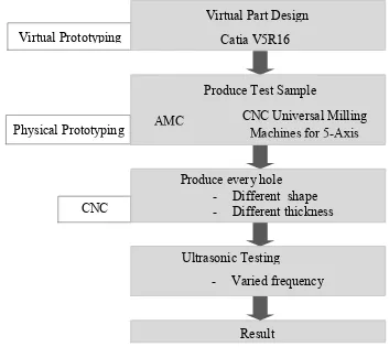
[image:35.612.131.484.311.626.2]Figure 3.2 below shows the flow process for research design. For test sample
virtual prototyping, Catia V5R16 software is used. Using an application of the same
software known as CATIA PROCESS, to do the programming for this test sample. The
physical prototyping is made using CNC Universal Milling Machines for 5-Axis which
is available in the Advanced Manufacturing Center (AMC). This test sample focuses on
different shape and thickness. Then, this test sample undergoes experiment using the
Ultrasonic Testing. These experiment objectives are to investigate the effect of probe
frequency and to investigate the effect of test sample material for probe frequency
selection.
Figure 3.2: Flow Process for Research Design
CNC
Result
Virtual Prototyping
Virtual Part Design
Catia V5R16
Physical Prototyping
Produce Test Sample
CNC Universal Milling
Machines for 5-Axis
AMC
Produce every hole
-
Different shape
-
Different thickness
Ultrasonic Testing
3.4
Design Analysis
There are four proposed test sample from the beginning of project till the last
submission which are accepted. The mainly focus of this design is to make artificial
defects which are different in size, shape and thickness. The design of the previous
design can be refer in Appendix 3A.
The material size for this test sample is 150x100x20.
The virtual prototyping of
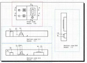
[image:36.612.157.502.345.595.2]the final design is made using Catia V5R16. This design vastly improves the previous
design especially in term of arrangement and purpose of the artificial defect. The
arrangement is important so that easy to use the UT. Fully design of this final test
sample can be refer in Appendix 3B.
Figure 3.3: Final Test Sample Drafting and Cross Section
industry. All of these cracks are varied to achieve different purpose. For the cross
section of this 6 cracks, please refer to appendix 3C.
[image:37.612.273.383.234.357.2]Four of these cracks are layered, which is purposely design to see the changes
signal at the different thickness. Beside that, to see either the vertical lines effect the
signal reading. Crack 2 is an example of layered crack which is shown in Figure 3.4
below.
Figure 3.4: Layered Crack
Some of the crack has a very small gap between each layer and the minimum of
the gap that are design in this test sample is 2 mm. The purpose of this small gap is to
see either the size of this gap effecting the reading and result of the UT.
One of the crack is design with the depth of 18 mm. However, the UT capability
to detect thickness is for minimum of 7 mm. So, this crack design is to show that the
capability of Ultrasonic Testing measurement for thickness that less than 7 mm. This
will give unclear signal where noise is near as a thickness.
A crack with chamfer is design to see the effect of this additional flat angle to the
result of UT. It is expected to see that when the probe reaches at the chamfer position,
display system will show an unclear signal.
3.5
Fabrication of Test Sample
Figure 3.5: CNC 5-Axis Face Milling (DMG-DMU250) [22]
Figure 3.5 above shows the CNC 5-Axis Face Milling that is used to fabricate the
test sample. This CNC machine is located at AMC. The information of this CNC 5-Axis
Face Milling can be referred in Appendix 3D. 5-Axis means that this machine has two
more axes in addition to three normal axis (XYZ) which allowing the horizontally
mounted workpiece to be rotated. This CNC system highly automated using CAD/CAM
programs. The programs produce a computer file that is interpreted to extract the
commands needed to operate a particular machine, and then loaded into the CNC
machines for production.
3F for H file. After the coding from H file is save in the CNC 5-Axis Face Milling, the
machining begun.
Both of aluminum and mild steel undergoes milling process. Figure 3.6 below
shows how the milling machine process is done. The type of machining operation that
done throughout this manufacturing is facing, pocketing, contouring and lastly surface
finish. There are four tools that been used, counterbore, ball nose and end mill toll size
Ø8 mm and Ø2 mm. Facing is done to machine the top face to provide the final
thickness of 20.00 mm, as per drawing. All of the cracks are done using pocketing
process. Contouring is done for filleted rectangular shape. Lastly, surface finish is a
compulsory for finishing. The machining process can be referred in Appendix 3G.
Figure 3.6: Milling Machining Process[23]
3.6
Ultrasonic Testing
3.6.1 Equipments
There are five basic equipments during Ultrasonic Testing Experiment. Which
are USD 30 ultrasonic flaw detector, 90° dual crystal probe with three different
frequency (2 MHz, 4 MHz and 5 MHz), test sample (mild steel and aluminum), lubricant
gel and IOW Calibration block. USD 30 ultrasonic flaw detector will give the result of
A-Scan. 90° dual crystal probe used as the type of probe because in theoretically, dual
crystal probe is better than single crystal because one for continually transmitting
ultrasonic waves and one for receiving. Test sample already fabricated is made by mild
steel and aluminum material. Lubricant gel is needed because solid to air interface
creates 100% reflection, so the sound goes straight back into probe without transmitting
into the metal. IOW Calibration steel block is important for calibrated for accurate
thickness measurement
Figure 3.7 below shows the equipment that use throughout Ultrasonic Testing
experiment. USD 30 ultrasonic flaw detector, 90° dual crystal probe, test sample and
couplant.
Figure 3.8: IOW Calibration Block
IOW Calibration Block that use during experiment is shown in Figure 3.8 above.
This Calibration Block is made from steel. Calibration is necessary every time the probe
is changed.
3.6.2 Procedure
The probe (2 MHz, 4 MHz, 5 MHz) is connected to the USD 30 and therefore an
ultrasonic beam was produced. First, using IOW Calibration block to calibrate. Some
lubricant gel is put on the surface of the block. The transducer is attached steadily and
softly on the lubricated surface and is moved towards edge of defect and stop when
significant echo is reached. The display system adjusted to A-scan display system. The
initial pulse set between 80-100% Full Screen Height (FSH) using the Gain Control.
Using pulse delay control, the initial transmission pulse is adjusted.
Figure 3.9: Reflected Sound Energy [24]
3.6.3 Parameter of Study
3.6.3.1 Objective: To investigate effect of probe frequency
Table 3.3: To Study Effect of Probe Frequency
Material
Frequency (MHz)
Parameter of Study
2
Pulse-Delay
Mild Steel
4
Gain
5
Sa
Table 3.3 above shows the parameter of study for effect of probe frequency. Mild
steel is used as the test sample. Three different frequency is used which is classified into
three class. Low (2 MHz), medium (4 MHz) and high (5 MHz). The result of the
experiment is A-scan graph that shows time base in x-axis and amplifier gain in y-axis at
the respective point. The important data that will be collected is pulse-delay, gain and
Sa.
3.6.3.2 Objective: To investigate the effect of test sample material for probe
frequency selection
Table 3.4: To Study the Effect of Test Sample Material for Probe Frequency
Selection
Frequency
(MHz)
Material
Material Velocity
(Mm/s)
Parameter of
Study
4
Mild Steel
Aluminum
5960
6400
Pulse Delay
Gain
Sa
CHAPTER 4
RESULT
4.1
Effect of Probe Frequency
An experiment for the effect of probe frequency has been conducted in the NDT
Lab. Probe frequency that used in this experiment are 2 MHz (low), 4 MHz (medium)
and 5 MHz (high). During this experiment, the parameters that will be control is the type
of probe, material of test sample and atmosphere condition. The type of probe that use
throughout this experiment is dual crystal probe. The test sample is made from mild
steel. The material velocity is set as 5960 Mm/s. Through out this experiment, some
steps are taken to avoid failure. The probe will be calibrated first using I.O.W steel
block. The initial pulse will be always set between 80-100% Full Screen Height (FSH).
FSH is the value of screen percentage. The probe will be moved towards edge of defect
and stop when significant echo is reach. Then, the display system shows the result that
discussed in this experiment for the effect of probe frequency, which is A-scan graph
that shows time base in x-axis and amplifier gain in y-axis at the respective point. The
defect echo feedback value will be search, and also the defect location will be detected.
noise detected quite high and all of the peak is quite width. The amplitude for the first
peak is 78% FSH. All of the general data is listed in Table 4.1.
Figure 4.1: 2 MHz Result for Backwall
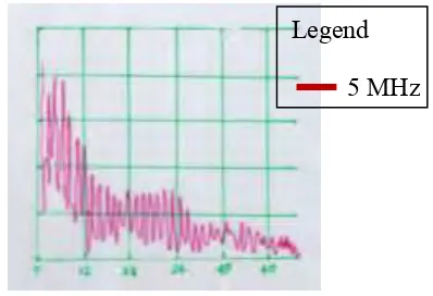
Figure 4.2 below shows the result for backwall signals in A-Scan for 4 MHz
probe. The initial pulse is roughly 96% FSH. There are 3 peaks that can be seen in this
60 mm full scale. The first backwall echo show that the value for Sa is 20.00 mm.
However from the graph, the noise detected is justifiable and all of the peak is sharper.
The amplitude for the first peak is approximately 62% FSH. All of the general data is
listed in Table 4.1.
Figure 4.2: 4 MHz Result for Backwall
Figure 4.3 below shows the A-Scan result for backwall signals of 5 MHz probe
frequency. The initial pulse is also approximately 90% FSH. There are 3 signals that can
be seen in this 60 mm full scale. The time base for this probe of the first back wall echo
Legend
2 MHz
Legend
value is 20.00 mm. However from the graph, the noise is little and the entire peak is
sharper. The amplitude for the first peak is around 41% FSH. All of the general data is
listed in Table 4.1.
Figure 4.3: 5 MHz Result for Backwall
Table 4.1: Result of Backwall for Different Probe Frequency
Frequency (MHz)
2
4
5
Material
Mild Steel
Gain (dB)
64.00
44.52
52.50
Pulse Delay (µs)
14.00
16.13
13.25
Sa (mm)
20.00
20.00
20.00
[image:46.612.271.382.570.667.2]Table 4.1 above shows the result of backwall analysis. From this table, the higher
frequency, lower the gain and pulse delay. However, for 4 MHz probe, the pulse delay is
higher than 2 MHz. All of the Sa value for backwall is 20.00 mm.
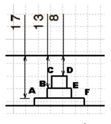
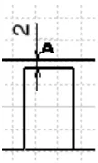
Figure 4.4: Crack 1 Cross Section
Legend
Figure 4.4 shows the cross section of Crack 1. Suppose when probe at the first
layer from A to B and C to D, the value of Sa will be 10 mm. The value Sa when the
probe move from B to C is 8 mm.
Figure 4.5 below shows the result for crack 1 signals the first layer of the crack,
which is from position A to B for 2 MHz probe. The initial pulse is roughly 88% FSH.
There are 6 peaks that can be seen in this 60 mm full scale. The first crack echo show
that the value for Sa is 10.00 mm. However from the graph, the noise detected is high
and most of the peak is width. The gain for the first peak is approximately 76% FSH. All
of the general data is listed in Table 4.2.
Figure 4.5: 2 MHz Result for Crack 1 at Position A to B
For 4 MHz probe, the result for back wall signals in A-Scan at the position from
A to B is as shown in Figure 4.6 below. The initial pulse is approximately 90% FSH.
There are 6 signals that can be seen in this 60 mm full scale. The first peak show that the
value for Sa is 10.00 mm. However from the graph, the noise detected is justifiable and
where not all peak is width. The amplitude for the first peak is 58% FSH. All of the
general data is listed in Table 4.2.
Legend
Figure 4.6: 4 MHz Result for Crack 1 at Position A to B
Figure 4.7 below shows the A-Scan result for back wall signals of 5 MHz probe
frequency. The initial pulse is also approximately 90% FSH. There are 6 signals that can
be seen in this 60 mm full scale. The time base for this probe of the first peak value is
10.00 mm. However from the graph, the noise is little and the entire peak is sharper. The
gain for the first peak is around 56% FSH. All of the general data is listed in Table 4.2.
Figure 4.7:
5 MHz Result for Crack 1 at Position A to B
Table 4.2 shows the result of Crack 1 at Position A to B general data analysis.
From this table, the higher frequency, lower the gain and pulse delay. All of the Sa value
for Back wall is 10.00 mm.
Legend
5 MHz
Legend
Table 4.2: Result of Crack 1 at Position A to B for Different Probe Frequency
Frequency (MHz)
2
4
5
Material
Mild Steel
Gain (dB)
60.50
55.00
46.50
Pulse Delay (µs)
15.77
13.09
12.93
Sa (mm)
10.00
10.00
10.00
Result of Crack 1 at position B to C for 2 MHz is shown in Figure 4.8 below.
The initial pulse is approximately 88% FSH. There are 8 peaks that can be seen in this
60 mm full scale. The first peak show that the value for Sa is 8.00 mm. However from
the graph, the noise detected quite high and all of the peak is quite width. The gain for
the first peak is 60% FSH. All of the general data is listed in Table 4.3.
Figure 4.8: 2 MHz Result for Crack 1 at Position B to C
Figure 4.9: 4 MHz Result for Crack 1 at Position B to C
For 4 MHz probe, the result for back wall signals in A-Scan at the position from
B to C is as shown in Figure 4.6 above. The initial pulse is approximately 86% FSH.
Legend
2 MHz
Legend
There are 5 signals that can be seen in this 60 mm full scale. The first peak show that the
value for Sa is 8.00 mm. However from the graph, the noise detected is acceptable and
where not all peak is width. The gain for the first peak is 58% FSH. All of the general
data is listed in Table 4.3.
Figure 4.10: 5 MHz Result for Crack 1 at Position B to C
Figure 4.3 above shows the A-Scan result for back wall signals of 5 MHz probe
frequency. The initial pulse is also approximately 82% FSH. There are 6 signals that can
be seen in this 60 mm full scale. The time base for this probe of the first peak value is
8.00 mm. However from the graph, the noise is little and the entire peak is sharper. The
gain for the first peak is around 54% FSH. All of the general data is listed in Table 4.3
below.
Table 4.3: Result of Crack 1 at Position B to C for Different Probe Frequency
Frequency (MHz)
2
4
5
Material
Mild Steel
Gain (dB)
59.00
55.00
43.00
Pulse Delay (µs)
15.77
13.18
12.58
Sa (mm)
8.00
8.00
8.00
Table 4.3 above shows the result of Crack 1 at Position B to C general data
analysis. From this table, the higher frequency, lower the gain and pulse delay. All of the
Sa value for first back wall echo is 8.00 mm.
Legend
When the probe moved from position C to D, the result for 2 MHz A-Scan is
shown in Figure 4.11 below. The initial pulse is approximately 92% FSH. There are 6
peaks that can be seen in this 60 mm full scale. The first peak show that the value for Sa
is 10.00 mm. However from the graph, the noise detected quite high and all of the peak
is width. The gain for the first peak is 62% FSH. All of the general data is listed in Table
4.4.
Figure 4.11: 2 MHz Result for Crack 1 at Position C to D
Figure 4.12 below shows the result of A-Scan for 4 MHz probe at Crack 1 at
position C to D. The initial pulse is roughly 92% FSH. There are 6 peaks that can be
seen in this 60 mm full scale. The first peak show that the value for Sa is 10.00 mm.
However from the graph, the noise detected is permissible and all of the peak is sharper.
The gain for the first peak is approximately 62% FSH. All of the general data is listed in
Table 4.4.
Figure 4.12: 4 MHz Result for Crack 1 at Position C to D
Legend
2 MHz
Legend
A-Scan result for crack 1 at position C to D for 5 MHz probe frequency is shown
in Figure 4.13 below. The initial pulse is also approximately 82% FSH. However, there
are only 4 peaks that can be seen in this 60 mm full scale. The time base for this probe of
the first peak value is 8.00 mm. However from the graph, the noise is little and the entire
peak is sharper. The gain for the first peak is around 54% FSH. All of the general data is
listed in Table 4.4 below.
Figure 4.13: 5 MHz Result for Crack 1 at Position C to D
Table 4.4: Result of Crack 1 at Position C to D for Different Probe Frequency
Frequency (MHz)
2
4
5
Material
Mild Steel
Gain (dB)
60.50
56.00
45.03
Pulse Delay (µs)
15.33
13.20
12.88
Sa (mm)
10.00
10.00
10.00
Table 4.4 above shows the result of Crack 1 at Position C to D general data
analysis. From this table, the higher frequency, lower the gain and pulse delay. All of the
Sa value for first crack echo is 10.00 mm.
Legend
The graph analysis and general data of result for crack 2, 4 and 5 are same as for
Crack 1. However, the only changes in this graph analysis is the crack echo value and
the noise. All of this A-Scan graph is asserted in the Appendix 4A.
However, there are some differences of A-Scan result for Crack 2 at position B
to C when using 5 MHz frequency. This result is shown in Figure 4.14 below.
Figure 4.14: 5 MHz Result for Crack 2 at Position B to C
[image:53.612.288.368.533.626.2]A-Scan result for crack 2 at position B to C for 5 MHz probe frequency is shown
in Figure 4.14 above. The initial pulse is approximately 90% FSH. The signal is quite
mess. The time base for this probe of the first peak value is suppose to be 13 mm, but the
value of Sa that achieved is 17 mm. All of the peak is sharp but the noise is regretfully
large that the crack echo is harder to read.
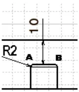
Figure 4.15: Cross Section of Crack 3
Figure 4.15 above shows the cross section of Crack 3 which have R2 chamfer.
Suppose when probe at the first layer from A to B, the value of Sa will be 10 mm.
Legend
For 2 MHz probe, the result for Crack 3 signals in A-Scan is as shown in Figure
4.16 below. The initial pulse is approximately 96% FSH. There are 3 peaks that can be
seen in this 60 mm full scale. The first peak show that the value for Sa is 10.00 mm.
However from the graph, the noise detected quite high and all of the peak is width. The
gain for the first peak is 48% FSH, with an amplitude that lower than the second peak.
All of the general data is listed in Table 4.5.
Figure 4.16: 2 MHz Result for Crack 3
For 4 MHz probe, the result for Crack 3 signals in A-Scan at the position from A
to B is as shown in Figure 4.17 below. The initial pulse is approximately 90% FSH.
There are 5 signals that can be seen in this 60 mm full scale. The crack echo show that
the value for Sa is 10.00 mm. However from the graph, the noise detected is acceptable
and where not all peak is width. The gain for the first peak is 58% FSH. However, the
first BWE echo is lower than second peak. All of the general data is listed in Table 4.5.
Figure 4.17: 4 MHz Result for Crack 3
Legend
2 MHz
Legend
Figure 4.18: 5 MHz Result for Crack 3
A-Scan result for crack 3 at position A to B for 5 MHz probe frequency is shown
in Figure 4.18 above. The initial pulse is also around 38% FSH. There are only 5 peaks
that can be seen in this 60 mm full scale. The time base for this probe of the first crack
echo value is 10.00 mm. From the graph, the noise is little and the entire peak is sharper.
However, the amplitude of the peak is cluttered. The gain for the first peak is around
54% FSH. All of the general data is listed in Table 4.5 below.
Table 4.5:
Result of Crack 3 at Position A to B for Different Probe Frequency
Frequency (MHz)
2
4
5
Material
Mild Steel
Gain (dB)
64.00
55.00
46.5
Pulse Delay (µs)
16.44
16.13
16.04
Sa (mm)
10.00
10.00
10.00
Table 4.5 above shows the result of Crack 3 at Position A to B general data
analysis. From this table, the higher frequency, lower the gain and pulse delay. All of the
Sa value for first BWE is 10.00 mm.
Figure 4.19 shows the cross section of Crack 6. With the size of 10 mmx10 mm,
this crack depth is 18 mm.
Legend
Figure 4.19: Cross Section for Crack 6
[image:56.612.255.452.288.428.2]When the probe moved to Crack 6, the result for 2 MHz A-Scan is shown in
Figure 4.20 below. The FSH value is 82%. The graph shows no crack echo due to the
noises. All of the general data is listed in Table 4.6.
Figure 4.20: 2 MHz Result for Crack 6
Figure 4.21 below shows the result for Crack 6 using 4 MHz probe frequency.
The noise is too high that no Sa reading can be figure
.
All of the general data is listed in
Table 4.6.
Figure 4.21: 4 MHz Result for Crack 6
Legend
2 MHz
Legend
The result of 5 MHz for Crack 6 is shown in Figure 4.22 below. The graph is
smoother but the Sa value still not shown. All of the general data is listed in Table 4.6
below.
Figure 4.22: 5 MHz Result for Crack 6
Table 4.6 below shows the result of Crack 1 at Position B to C general data
analysis. From this table, the higher frequency, lower the gain and pulse delay. There is
no Sa value detected.
Table 4.6:
Result of Crack 1 at Position C to D for Different Probe Frequency
Frequency (MHz)
2
4
5
Material
Mild Steel
Gain (dB)
40.00
46.5
47.00
Pulse Delay (µs)
16.55
16.17
13.00
Sa (mm)
-
-
-
Legend
4.2
The Effect of Test Sample Material for Probe Frequency Selection
To investigate the effect of test sample material for probe frequency selection, an
experiment has been conducted in the NDT Lab. To meet the objective of the
experiment, the probe frequency that used in this experiment is 4 MHz only. This is
because to see either the 4 MHz is more suitable for mild steel or aluminum. Beside
probe frequency, the parameters that will be control is the type of probe and atmosphere
condition. The type of probe that use throughout this experiment is still dual crystal
probe. However, the test sample is made from mild steel and aluminum. The material
velocity is set to be 6400 Mm/s. Throughout this experiment, some steps are taken to
avoid failure. The probe will be calibrated first using I.O.W steel block. The initial pulse
will be always set between 80-100% FSH. The probe will be moved towards edge of
defect and stop when significant echo is reach. Then, the display system shows the result
that discussed in this experiment for the effect of probe frequency, which is A-scan
graph that shows time base in x-axis and amplifier gain in y-axis at the respective point.
The defect echo feedback value will be search, and also the defect location will be
detected.
Figure 4.23: 4 MHz Result for Aluminum Backwall
[image:59.612.124.521.369.656.2]Table 4.7 below shows the result of backwall analysis for mild steel and
aluminum material when using the same probe frequency, which is 4 MHz. It is shows
that aluminum use lower gain and pulse delay from mild steel.
Table 4.7: Result of Backwall for Mild Steel and Aluminum
Frequency (MHz)
4
Material
Mild Steel
Aluminum
Gain (dB)
44.52
33.50
Pulse Delay (µs)
16.13
15.40
[image:59.612.182.431.426.654.2]Sa (mm)
20.00
20.00
Figure 4.24: 4 MHz Result for Aluminum for Crack 1 at Position A to B
Legend
4 MHz
Legend
Crack 1 result for mild steel test sample is in Figure 4.6. While result of the
aluminum test sample is shown in Figure 4.24 above. The initial pulse is roughly 90%
FSH. There are 5 peaks that can be seen in this 60 mm full scale. The first crack echo
show that the value for Sa is 10.00 mm. However from the graph, the noise detected is
justifiable and all of the peak is sharp. However the gain for first peak is short, around
42% FSH. All of the general data is listed in Table 4.8.
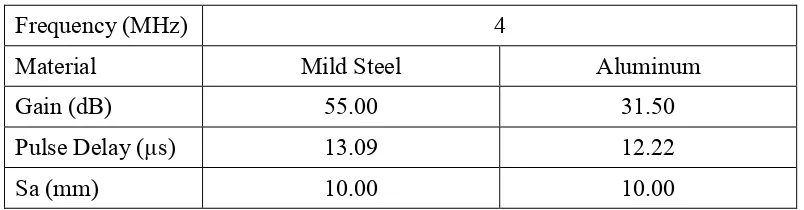
[image:60.612.127.529.317.422.2]Table 4.8 below shows the result of crack 1 analysis for mild steel and aluminum
material when using the same probe frequency, which is 4 MHz. It is shows that
aluminum use lower gain and pulse delay from mild steel.
Table 4.8: Result of Crack 1 at Position A to B for Mild Steel and Aluminum
Frequency (MHz)
4
Material
Mild Steel
Aluminum
Gain (dB)
55.00
31.50
Pulse Delay (µs)
13.09
12.22
Sa (mm)
10.00
10.00
[image:60.612.185.404.522.659.2]All of A-Scan result characteristic and general data for each crack and point is
nearly identical with an exception of Crack 3 and 6. All experiment result in term of
A-Scan graph is asserted in Appendix 4.
Figure 4.25: 4 MHz A-Scan Result for Aluminum at Crack 3
Legend
For Crack 3, the result of Crack 3 signals in A-Scan is as shown in Figure 4.25
above. The initial pulse is around 90% FSH. There are 3 peaks that can be seen in this
60 mm full scale. The first crack echo shows that the value for Sa is 10.00 mm. However
from the graph, there are some unsignificant signal, probably noise and the peak is
sharp. The gain for the first peak is 49% FSH, with an amplitude that slightly lower than
the second peak. All of the general data is listed in Table 4.9.
Table 4.9: Result of Crack 1 at Position A to B for Mild Steel and Aluminum
Frequency (MHz)
4
Material
Mild Steel
Aluminum
Gain (dB)
55.00
32.00
Pulse Delay (µs)
16.13
11.68
Sa (mm)
10.00
10.00
[image:61.612.185.404.460.598.2]The result of aluminum material for Crack 6 is shown in Figure 4.26 below. The
graph is smoother but the Sa value still not shown. All of the general data is listed in
Table 4.10 below.
Figure 4.26: 4 MHz A-Scan Result for Aluminum at Crack 6
Table 4.10 shows the result of crack 6 analysis for mild steel and aluminum
material when using the same probe frequency, which is 4 MHz. It is shows that
aluminum use lower gain and pulse delay from mild steel.
Legend
Table 4.10: Result of Crack 6 for Mild Steel and Aluminum
Frequency (MHz)
4
Material
Mild Steel
Aluminum
Gain (dB)
46.5
36.00
Pulse Delay (µs)
16.17
11.00
Sa (mm)
-
-
4.3
Crack Location
The test sample is drawn into grid of 10 mmx10 mm. The probe then will be
moved along the grid line and each time the signals change, the spot will be marked.
After that, the probe is slowly moved in each grid until the shape of crack defined.
Figure 4.27: Crack Location and Shape
Legend
X 2 mm
X 8 mm
X 10 mm
X 12 mm
CHAPTER 5
DISCUSSION
5.1
Introduction
From the experiment, the probe frequency that will be used are 2 MHz, 4MHz
and 5 MHz. This is because the probes are available from NDT Lab in Universiti
Teknikal Malaysia Melaka. This probe frequencies are categorized in three classes;
which are high (5 MHz), medium (4 MHz) and lastly low (2 MHz). It is important to
study the effect of the probe frequency from low to high signal. In this chapter, the result
of two experiment will be discussed in details. The first experiment is to investigate the
effect of probe frequency and the second experiment is to the effect of test sample
material for probe frequency selection
5.2
Effect of Probe Frequency
pulse are 96% FSH. So, it can be assumed that due to the initial pulse being too high,
the result of gain and back pulse of 4 MHz is affected.
Figure 5.1: Graph Gain & Pulse Delay Versus Frequency for Backwall
To compare the effect of probe frequency, the A-Scan result is trace using
transparent paper. This overlapping A-Scan is to compare the effect of frequency
between 2 MHz and 5 MHz. Black line indicates Scan of 2 MHz while red line is
A-scan for 5 MHz.
Figure 5.2: A-Scan Backwall for 2 MHz and 5 MHz
From Figure 5.2 above, it is observed that both of 2 MHz and 5 MHz have the
same thickness of 20.00. From the observation, all of 2 MHz peaks is wider than 5 MHz
Legend
2 MHz
[image:64.612.202.415.492.629.2]so, the peak for 5 MHz is sharper than 2 MHz. However, the amplitude for 5 MHz is
lower than 2 MHz. The noise is high for 2 MHz compare to 5 MHz.
All of the graph for every crack and position is similar to the Figure 5.2 in terms
of the width, amplitude and noise differences. All of this A-Scan result for 2 MHz and 5
MHz can be referred to in Appendix 5A.
The width of the peak is effected by beam that produce by transducer. 5 MHz has
a sharper peak than 2 MHz because higher frequency produce a narrow, well defined
beam.
The higher the test frequency, the greater attenuation and the less penetration that
can be achieved. So, the amplitude of the 5 MHz is supposed to be lower than 2 MHz
because of the less penetration that achieved by it.
Noise occurred when scattered energy (sound to reflect in random direction due
to grain boundaries in material) reach to receiver. Scatter decrease if frequency
decreased. However a higher frequency will result in higher attenuation. Even though
this attenuation limit the range of higher frequency, but the noise at the same higher
frequency is also less. Beam angle also helps to lower background noise interference by
limiting the probe’s noise sensitivity to area defined by the angle of the sensor. The
result that shows 2 MHz have more noise than 5 MHz in Figure 5.2 is proven.
Figure 5.3: Graph Gain & Pulse Delay Versus Frequency for Crack 1 at Position A to B.
5.3
Effect of Test Sample Material for Probe Frequency Selection
From Back wall general data, the chart for gain and pulse delay are made in
Figure 5.4 below. This chart shows that aluminum has lower gain and pulse delay than
mild steel.
0
10
20
30
40
50
Mild Steel
Aluminum
Material
Gain & Pulse Delay for Different Material
[image:66.612.164.446.522.643.2]Gain (dB)
Pulse Delay (µs)
To compare the effect material for probe frequency selection, the A-Scan result is
trace using transparent paper. This overlapping A-Scan is to compare result between
mild steel and aluminum using the same frequency, 4 MHz. Blue line indicates A-Scan
for mild steel while red line is A-scan for aluminum.
Figure 5.5: A-Scan Backwall for Mild Steel and Aluminum
Figure 5.5 above shows the A-Scan backwall for mild steel and aluminum.
However, the signals for backwall in Figure 5.5 above show little differences. It can be
seen that most of mild steel BWE is wider than aluminum so, the peak for aluminum is
sharper than mild steel. The amplitude for aluminum is lower than mild steel.
Both of these observations, chart in Figure 5.4 and graph in Figure 5.5 proved that
material factors effecting probe frequency selection. The ultrasonic sound beam
propagation is influenced by grain type, size and distribution of material. Large or
directionally oriented grains tend to scatter and otherwise absorb ultrasonic energy to a
greater extent than fine, randomly oriented grains. Beside that, another factor for this
experiment is the surface condition for test sample. Example surface condition will be
considered during this experiment is corrosion, surface roughness
Mild steel grain size is considered to be larger than aluminum and mild steel also
known for its poor corrosion resistance. So, theoretically, aluminum will have sharper
and narrow signals, less noise and high amplitude from mild steel. Mild steel also will
have less peak from aluminum. However, the result in Figure 5.5 shows that aluminum
has higher amplitude, this probably due to some error during the experiment. Most of
Legend
Mild Steel
result for experiment the effect of test sample material for probe selection shows the
exact outcome as theoretically.
Figure 5.6 shows the A-Scan result for mild steel and aluminum at Crack 1 when
positioned from A to B. Clearly, mild steel peak is wider than aluminum so, the peak
for aluminum is sharper than mild steel. The amplitude for aluminum is higher than mild
steel. This is example of the correct result suppose to get in theoretically.
Figure 5.6
:
A-Scan Crack 1 at Position A to B for Mild Steel and Aluminum
5.4
Design Factor
Crack shape and size affecting the reading of Ultrasonic Testing. After the
experiment is done using mild steel test sample, the suitable probe frequency will be
chosen specifically to each defect. This is the conclusion of probe frequency selection
for type of defect.
Crack 2 has a very small gap at position B to C and D to E, which is only 2 mm.
The purpose of this small gap is to see either the size of this gap effecting the reading
and result of the UT. During the experiment, to achieve the result of A-scan that
acceptable is hard due to its location, in the centre of three layered crack and gap for 2
mm only.
Legend
Mild Steel
Figure 5.7: A-Scan Crack 2 at Position B to C for 2 MHz and 5 MHz
The Figure 5.7 before shows the result of A-Scan Crack at Position B to C for 2
MHz and 5 MHz. Although the graph for 2 MHz has more noises, the right value Sa
which is 13 mm still can be detected. In contrast, the 5 MHz did detect this crack, but the
Sa that considered in this experiment is 17 mm. This experiment has proved that, low
frequency is more suitable to detect small size defect. When frequency increased,
attenuation will be increased too. Then, this lead to less penetration can be achieved. So,
smaller size defects harder to achieve.
A crack with chamfer is design to see the effect of this additional flat angle to the
result of UT. It is expected to see that when the probe reaches at the chamfer position,
display system will show an unclear signal.
Figure 5.8: A-Scan at Crack 3 for 2 MHz and 5 MHz
Legend
2 MHz
5 MHz
Legend
2 MHz
Figure 5.8 shows the result of A-Scan at Crack 3. From the graph, 2 MHz did not
achieved the Sa value 10 mm but 20 mm. However, the noise is still acceptable even for
2 MHz. This probably due to the radius of chamfer is small. It is suggested that in this
situation, higher frequency should be use. This is due to the attenuation that reduce the
noise.
Crack 4 designed to be rounded. Purpose of this design is to show the effect for
different type of crack. From theory, the square shape will give clearer signal because of
the flat wall while the rounded crack is not. This graph can be refer in Appendix 4A.
One of the crack is design with the depth of 18mm. Supposedly, UT can detect
thickness with minimum of 7 mm. So, this crack design is to show that the capability of
Ultrasonic Testing measurement for thickness that less than 7 mm. All of results showed
unclear signal where noise is near as a thickness. However, the result for A-Scan at
Crack 6 for 2 MHz and 5 MHz still be compared in Figure 5.10 below.
Figure 5.9: A-Scan at Crack 6 for 2 MHz and 5 MHz
From the Figure 5.8 above, even though both of the probe frequency shows
unclear signal, but the 5 MHz graph shows smoothe