Assessing the inner core nucleation paradox with atomic-scale simulations

Contents lists available atScienceDirect

Earth

and

Planetary

Science

Letters

www.elsevier.com/locate/epsl

Assessing

the

inner

core

nucleation

paradox

with

atomic-scale

simulations

Christopher

J. Davies

a

,

∗

,

Monica Pozzo

b

,

Dario Alfè

b

,

c

a_{SchoolofEarthandEnvironment,UniversityofLeeds,LeedsLS29JT,UK}

b_{DepartmentofEarthSciencesandThomasYoungCentre@UCL,UCL,GowerStreet,WC1E6BT,London,UK} c_{LondonCentreforNanotechnology,UCL,GowerStreet,WC1E6BT,London,UK}

a

r

t

i

c

l

e

i

n

f

o

a

b

s

t

r

a

c

t

Articlehistory:

Received22June2018

Receivedinrevisedform29September 2018

Accepted11November2018 Availableonline3December2018 Editor:B.Buffett

Keywords:

Earthcore innercorefreezing atomic-scalesimulations homogeneousnucleation classicalnucleationtheory

WeinvestigatetheconditionsrequiredtofreezeliquidironandironalloysnearthecentreofEarth’score. Itisusuallyassumedthatinnercoregrowthbeginsoncetheambientcoretemperaturefallsbelowthe melting temperatureofthe ironalloyatEarth’scentre;however,additional (under)coolingis required to overcomethe energybarrierassociated withcreating asolid–liquidinterface.Predictionsbasedon ClassicalNucleationTheory(CNT)haveestimatedarequiredundercoolingof∼1000 K,whichcannotbe reconciledwithpredictedcorecoolingratesof∼100 K Gyr−1_{.Thisapparentcontradictionhasbeencalled} the‘innercorenucleationparadox’.HereweaddressthreemajoruncertaintiesintheapplicationofCNT toinnercorenucleationusingatomic-scalesimulations.First,wesimulatefreezinginFeandFe–Oliquids atcoreconditionstoself-consistently constrainallparametersrequiredbytheCNT equations.Second, we test the basicvalidity ofCNT bydirectly calculatingthe waiting time toobserve freezing events inFeandFe–Oliquids.Third,weinvestigatetheinfluenceofwave-likeforcings appliedtotheatomic simulations,whichhavebeensuggestedasameanstosignificantlyreducetheenergybarrier.Ourresults areconsistentwithCNTinthecomputationallyaccessibleparameterregime,thougherrorestimateson the waiting timecan reach 50%of themeasurement atthe largest undercooling temperatures. Using CNT toextrapolatetoinner coreconditions yieldsestimatedundercooling of730±20 Kfor thepure ironsystemand675_±35 KfortheFe–Osystem.Forcingscorrespondingtolargepressurevariationsof

O(10)GPareducethesevaluesby∼100 K.Whileourundercoolingestimatesaresignificantlylowerthan previousestimatestheyarenotlowenoughtoresolvetheinnercorenucleationparadox.

©2018TheAuthors.PublishedbyElsevierB.V.ThisisanopenaccessarticleundertheCCBYlicense (http://creativecommons.org/licenses/by/4.0/).

1. Introduction

The formation of the solid inner core was a defining moment in Earth’s history. Continual freezing of the liquid core releases latent heat and lighter elements, the latter providing the gravitational energy that is the main power source maintaining the present ge-omagnetic field (Braginsky, 1963; Gubbins, 1977; Nimmo, 2015). Prior to inner core formation, higher cooling rates are needed to explain the existence of the geomagnetic field for the last 3.5 Ga (Tarduno et al., 2010). If the inner core is 400–700 Myrs old, as suggested by high core thermal conductivity values (Pozzo et al., 2012; de Koker et al., 2012; Gomi et al., 2013), then conventional thermal history models predict early core temperatures far above current estimates of the lower mantle solidus (Nimmo, 2015; Davies et al., 2015; Labrosse, 2015), implying widespread

melt-*

Correspondingauthor.

E-mailaddress:c.davies@leeds.ac.uk(C.J. Davies).

ing in early times. However, some studies have suggested that this rapid cooling scenario is unsustainable and argue that novel crys-tallization mechanisms powered the early magnetic field (O’Rourke and Stevenson, 2016; Badro et al., 2016; Hirose et al., 2017), slow-ing core coolslow-ing and allowslow-ing an inner core age of

>

1 Ga, though the efficiency of these processes has been questioned (Du et al., 2017). Clearly, the preferred scenario depends critically on the age of the inner core.

All current core thermal history models assume that the inner core nucleates when the melting curve for the liquid iron alloy falls below the core (adiabatic) temperature at Earth’s centre (e.g. Nimmo, 2015; Davies, 2015; Labrosse, 2015). However, freezing of solid from liquid requires the creation of a solid–liquid interface, with an associated free energy barrier. The size of the barrier is determined by the competition between the (negative) volumetric and (positive) interfacial free energy; the top of the barrier corre-sponds to the critical radius, beyond which crystals will continue to grow (e.g. Christian, 2002). The time required for crystals to reach the critical radius is infinite if the system is at the

melt-https://doi.org/10.1016/j.epsl.2018.11.019

ing temperature and therefore some undercooling is needed for the system to reach equilibrium with solid as the stable phase below the melting temperature. The effect of undercooling is to delay the onset of inner core nucleation compared to predictions from existing models; larger undercooling leads to greater delay. Determining the amount of undercooling is therefore crucial for predicting the inner core age, which in turn impacts estimates of the power available to the dynamo and the thermal evolution of the core.

Consequences of undercooling at the inner core boundary (ICB) have long been discussed, mainly in connection with the possi-ble existence of a mushy zone ahead of the ICB (e.g. Loper and Roberts, 1977; Fearn et al., 1981). Shimizu et al. (2005) used classi-cal nucleation theory (CNT) to investigate the formation of crystals in a slurry layer above the ICB. They found that the probability of forming a slurry by homogeneous nucleation (nucleation in the absence of solid surfaces) would be essentially zero and suggested that nucleation must begin heterogeneously (i.e. on a pre-existing surface). Huguet et al. (2018) used CNT to investigate the origin of the inner core and found that a critical undercooling

δ

Tc

∼

1000 K

is needed to bring the waiting time for generating a stable nu-cleus below O

(

1

)

Gyr. Since the core is cooling at O

(

100

)

K Gyr−1 (Davies, 2015), such a large

δ

Tc is clearly impossible. Moreover,

upon reaching an undercooling of

∼

1000 K most of the core would rapidly freeze since a large region would be below the melting point. The existence of the inner core coupled with the apparently impossibility of homogeneously nucleating solid near Earth’s cen-tre led Huguet et al. (2018) to label the problem the ‘inner core paradox’.

Huguet et al. (2018) considered several limitations of CNT, but still found that homogeneous nucleation cannot explain inner core nucleation. They considered various catalysts for heterogeneous nucleation, all with caveats; the least implausible scenario was considered to be delivery of solid to Earth’s centre from the man-tle. The difficulty here is that the solid must be dense enough to sink to Earth’s centre, which requires that it is composed of pure iron or iron alloyed with an element that is heavier than the main light elements in the core, thought to be silicon, sulphur and oxy-gen (Alfè et al., 2002b; Hirose et al., 2013). All viable alloys are thought to be highly soluble in liquid iron and so the solid would need to be large enough to avoid complete dissolution in either the lower mantle or core during its descent. Given the significant uncertainties with the existence and dynamics of this process it cannot be yet be considered a robust explanation for the inner core paradox.

In this paper we address three major uncertainties involved in the application of CNT to inner core nucleation using molecu-lar dynamics simulations. First, we calculate the quantities needed to evaluate CNT for pure iron and iron alloys at core conditions. Huguet et al. (2018) were forced to use highly uncertain estimates for the prefactor I0 and interfacial energy

γ

(defined precisely

be-low) required by the CNT equations since relevant estimates for iron alloys were not available. We focus on iron–oxygen alloys since O does not enter the solid at core conditions (Alfè et al., 2002b) and is therefore the element primarily responsible for the seismically-observed density difference between the solid and liq-uid core and the 600–700 K depression in the core melting temper-ature compared to the melting temperature of pure iron (Davies, 2015).

Second, we test the basic validity of CNT at core conditions us-ing two sets of simulations for each composition. In the first set we model freezing from a pure liquid and calculate the waiting time required to observe freezing events for a given undercooling with-out recourse to CNT. In the second set we model freezing from a seed, which is much less computationally demanding but requires CNT to relate the undercooling to the waiting time.

Third, we investigate the effect of external wave-like forcings applied to our simulations. Previous studies have found that such forcings can significantly reduce the nucleation barrier (see Huguet et al., 2018, for a discussion). A wide variety of waves exist in the liquid core, ranging from slow waves that arise from magnetic and rotational effects to seismic and electromagnetic waves (Moffatt, 1978). We consider an arbitrary forcing with prescribed amplitude that is not directly related to a particular wave-like motion in the core. The goal at this stage is simply to understand whether a wave-like forcing can reduce the undercooling for core materials at core conditions.

This paper is organised as follows. In Section 2we present rel-evant results from CNT and describe the atomic potentials used in our calculations of the Fe and Fe–O liquid systems. In Section3we present results for nucleation from a pure liquid and nucleation in the presence of a solid seed in both Fe and Fe–O systems and com-pare the results to CNT. We discuss the application of these results to Earth in Section4and provide conclusions in Section5.

2. Methods

2.1. Classicalnucleationtheory

At equilibrium a thermodynamic system is found in the state of minimum Gibbs free energy g. In particular, equilibrium between a solid and a liquid is obtained at the melting temperature Tm,

where gsl

=

gs

−

gl

=

0, with gs and gl the free energies of solid and liquid, respectively. If a liquid is cooled below Tmit will

even-tually solidify, but homogeneous solid nucleation is an activated process, because the formation of a solid embryo inside the liquid introduces a solid–liquid interface, with an associated positive free interfacial energy

γ

. The process is usually described by classical nucleation theory (CNT) (Christian, 2002). If the embryo is spher-ical with radius r then the Gibbs free energy change as it forms is:

G

=

4

3

π

r

3_gsl

₊

₄

_π

_r2

_γ

_.

₍₁₎

The number of embryos I

(

r

)

formed in the liquid per unit volume per unit time is proportional to exp

(

−

G

/

kBT

)

, where kB is the

Boltzmann constant and T is the temperature.

Above Tm both terms in equation (1) are positive and so

G

increases with r. The distribution of embryos is therefore confined to small radii, as the probability of forming an embryo of radius r is a decreasing function of r. Below Tm the first term in

equa-tion (1) is negative, and therefore

G increases at first, reaches a maximum, and then decreases monotonically. If we define rc to be

the critical embryo radius corresponding to the maximum of

G, then I

(

rc

)

is minimum and an embryo of that size will be unstable,

having equal probability of either remelting or growing. If the em-bryo starts to grow beyond rc, the probability of growing further

increases exponentially, and the whole system solidifies.

The condition to determine rc is obtained by setting d

G

/

dr

=

0, which gives rc

= −

2

γ

/

gsl. Near Tm we can write:

gsl

hf

δ

T Tm

hc

(δ

T

),

(2)

where hf is the enthalpy of fusion,

δ

T

=

T

−

Tm is the

undercool-ing and hc

(δ

T

)

is a correction that accounts for the non-linear

be-haviour of the solid–liquid free energy difference as

δ

T increases. In standard CNT hc

=

1, but we found that for

δ

T

∼

1000 K hc can

be as large as 1

.

06 and is therefore not completely negligible. By analysing our free energy data for pure iron (Alfè et al., 2002c) we found that a correction of the type hc

(δ

T

)

=

1

−

7

.

046

×

10−5

×

δ

T

equation (2) to less than 1% up to

δ

T

= −

2000 K. Note that the correction is positive, meaning that the same value of

G is ob-tained for somewhat lower

δ

T.

The critical radius can thus be re-written as

rc

−

2

γ

Tm hfhc

(δ

Tc

)δ

Tc

,

(3)

and is therefore a function of the interfacial energy

γ

and the crit-ical undercooling temperature

δ

Tc: the closer the temperature to

Tm the larger the critical radius. By substituting equations (2) and

(3) into equation (1) we obtain the value of the height of the free energy barrier to nucleation:

Gc

=

16 3

π γ

3T_m2

δ

Tc2h2_f

[

hc

(δ

Tc

)

]

2

.

(4)

The number of embryos of critical size rc per unit volume per unit

time is

I

=

I0exp

−

16

3

π γ

3_T2

m kBT

δ

Tc2h2f

[

hc

(δ

Tc

)

]

2

,

(5)

where I0 is a prefactor which is related to the number of atoms

per unit volume and an attempt frequency of bringing atoms to-gether to form a solid embryo.

Since they are at the top of the free energy barrier, on average half of these embryos will re-melt, and the other half will grow and lead to a freezing event.1_{The average waiting time to observe} a freezing event,

τ

v (units of s m3), is therefore

τ

v

=

1 2I0

exp

16 3

π γ

3_T2

m kBT

δ

T2ch2f

[

hc

(δ

Tc

)

]

2

.

(6)

This discussion suggests two possible ways to study homoge-neous freezing via molecular dynamics simulation: freezing from a pure liquid and freezing with a seed. In each case we consider both pure iron and iron–oxygen alloys. In the case of freezing a pure liquid, described in Section 3.1, we simulate the liquid at different temperatures below the melting temperature until it freezes and measure the time for these freezing events to occur. This method provides a direct test of CNT using equation (6). In the case of freezing with a seed, described in Section3.2, we fix the seed size and vary temperature until the seed melts. This method does not directly test CNT via equation (6); instead it tests the linear rela-tion given by equation (3), which can be used to infer

γ

. In the following two subsections we describe the technical details of the pure iron and the iron oxygen potentials, including the prediction of their melting properties.

2.2.Pureiron

In the pure iron system we use an embedded atom model (EAM) (Daw and Baskes, 1983; Sutton and Chen, 1990) developed in Alfè et al. (2002a), in which the total energy has the form

Etot

=

i

Ei

,

(7)

where the atomic energies Eiconsist of two parts:

Ei

=

Erepi

+

F

(

ρ

i

)

=

i<j

(

a

/

ri j

)

n

−

C

ρ

i1/2

.

(8)

1 _{Inrealitytheprobabilityofre-meltingorgrowingintoalargersolidarenot}

ex-actlyequal,asthefreeenergyprofileinequation (1) isnotsymmetricwithrespect torc,butdeviationswillonlymarginallyaffectthepre-factorandcanbeignored.

Here Erep_i is a purely repulsive function of the interatomic dis-tances ri j and F

(

ρ

i

)

is an embedding term accounting for the

metallic bonding, with the densities

ρ

i

=

j=i

(

a

/

ri j

)

m. The

val-ues of the parameters are: n

=

5

.

93

,

=

0

.

1662 eV, C

=

16

.

55, a

=

3

.

4714 Å and m

=

4

.

788 (Alfè et al., 2002a). We performed simu-lations with two system sizes, including 7776 and 40960 atoms. The volume was 7

.

04285 Å3/atom, giving pressures p close to 323 GPa at the temperatures of interest. We prepared the systems by melting and equilibrating them close to the melting tempera-ture. These initial configurations were then given random velocities drawn from a Maxwellian distribution. All simulations were per-formed in the microcanonical ensemble (constant number of atoms N, constant volume V and constant energy E), using the Verlet al-gorithm with a time step of 1 fs. We extended each simulation by up to 2 ns, which resulted in a maximum accumulation of the drift in the constant of motion of no more than 10 K.

2.3. Iron–oxygenmixtures

To simulate iron oxygen mixtures we have constructed a more general EAM potential of the form

Etot

=

iFe EiFe

+

iO EiO

+

iFeO

EiFeO

,

(9)

where iFeruns over the iron atoms, iOover the oxygen atoms and iFeOover the whole list of atoms. The atomic energies are

EiFe

=

E

rep

iFe

+

FFe

(

ρ

iFe

)

=

i<j

(

a

/

riFejFe

)

n

₋

_C

_ρ

1/2

iFe

,

(10)

EiO

=

E

rep

iO

+

FO

(

ρ

iO

)

=

i<j

O

(

aO

/

riOjO

)

nO

−

OCO

ρ

_i1_O/2

,

(11)

and

EiFeO

=

E

rep

iFeO

=

1

/

2

iFe=jO

FeO

(

aFeO

/

riFejO

)

nFeO

_,

₍₁₂₎

with densities

ρ

iFe

=

jFe=iFe

(

a

/

riFejFe

)

m

₊

jO

(

aFeO

/

riFejO

)

mFeO ₍₁₃₎

and

ρ

iO

=

jO=iO

(

aO

/

riOjO

)

mO

+

iFe

(

aFeO

/

riFeiO

)

mFeO ₍₁₄₎

The bonding term FOis not essential, but we keep it for generality.

To obtain the values of the parameters we used a 30 ps tra-jectory in a system containing 127 iron and 30 oxygen atoms at a temperature of 6350 K and a pressure of 240 GPa using den-sity functional theory (DFT). The simulation was performed with the vasp code (Kresse and Furthmüller, 1996) using the techni-cal parameters in Davies et al. (2018). The accuracy of the DFT description of iron at Earth’s core conditions has been demon-strated in previous work, which showed good predictive power for its high pressure static, dynamic and thermodynamic prop-erties (Alfè et al., 2000, 2001, 2002a; Gillan et al., 2006). We extracted Nl

=

6000 configurations (one every 5 fs) and

calcu-lated DFT energies U

(

l

)

and pressures p

(

l

)

for each configurationl. With these we constructed the quantities

δ

U

(

l

)

=

Etot

(

l

)

−

U

(

l

)

and

δ

p

(

l

)

=

pEAM

(

l

)

−

p

(

l

)

, where pEAM

(

l

)

is the pressure computed

with the EAM model. The parameters of the EAM were then ob-tained by minimising the quantities

δ

U2

=

1

/

Nl

l

(δ

U

(

l

)

−

δ

U

)

2

,

δ

U

=

1

/

Nl

l

[image:4.612.322.533.55.204.2]

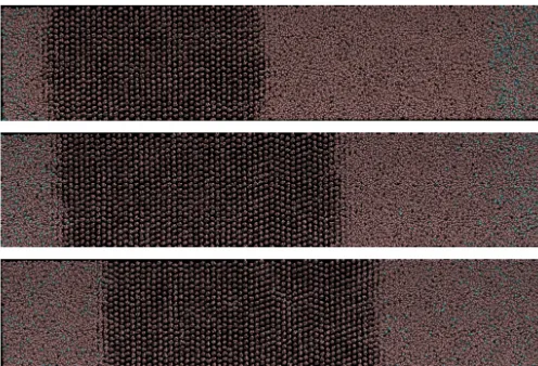
Fig. 1.Exampleofsolid–liquidcoexistenceinaniron–oxygenmixtureatapressure of323GPa.Initially,the cellisbuiltwithsolidandliquid ironincoexistenceat thepureironmeltingtemperatureof6215K.Thesimulationisthenstopped,1000 ironatoms(outofatotalof40,000)intheliquidaretransformedtooxygens(blue dots),andthesimulationisresumedwithnewrandomvelocities(toppanel).Inthis particularexamplethevelocitiesaredrawnfromaMaxwelliandistributionwitha temperatureof5000K.Sincethetotalenergyofthesystemhasbeenreduced,the pureironpartofthecellstartstofreeze(middle),andthereleaseoflatentheat increasesthe temperature.Thetemperatureisabovethemeltingtemperatureof themixture,andthisstartstomelt(leftsideofthecell),whilethepureironside ofthecellkeepsfreezinguntilthetemperaturereachesthemeltingtemperatureof themixture(bottom).Thesnapshotsaretakenatt=0,0.1,0.3 ns,respectively.(For interpretationofthecoloursinthefigure,thereaderisreferredtothewebversion ofthisarticle.)

and

δ

p2

=

1

/

Nl

l

(

pEAM

(

l

)

−

p

(

l

))

2

.

(16)

The value of the parameters n,

, C, a, and m were left un-changed to those of the pure iron system. The other parame-ters were nO

=

9

.

17,

O

=

0

.

0885 eV, C

=

16

.

4, aO

=

2

.

602 Å, mO

=

7

.

483, nF e O

=

4

.

796,

F e O

=

0

.

2172 eV, aF e O

=

3

.

408 Å and

mF e O

=

4

.

731. With these parameters the mean root square of the

fluctuations in the energy differences is

δ

U2

_/

_k

BT

=

0

.

36, which

is about 50% larger than the value found for the EAM for pure iron, but still small.

2.4. Iron–oxygenmeltingpointdepression

To study the waiting time as a function of undercooling in the Fe–O system we first computed Tm as a function of oxygen

con-centration. We used the coexistence approach, in which solid and liquid are simulated side by side in a large simulation cell contain-ing 40,000 atoms in the NVE ensemble. Startcontain-ing with the pure iron system to establish solid–liquid coexistence, we then transmuted 1000 iron atoms into oxygen in a portion of the liquid neigh-bouring the solid on one side (see Fig.1(a)) and removed some kinetic energy from the system by restarting the simulation with lower velocities. This process causes the temperature to fall below the melting temperature of the pure system and the iron solid– liquid interface to move into the liquid as the solid phase grows (Fig. 1(b)), while oxygen also starts to diffuse in the liquid. Re-lease of latent heat causes the system to heat up: solid continues to grow on the pure iron side of the simulation, which remains below its melting temperature, while solid iron neighbouring the liquid–oxygen mixture starts to melt due to the reduced melting temperature (Fig.1(c)). Once oxygen is well mixed throughout the liquid and the temperature has settled to the melting temperature of the mixture the system reaches equilibrium, with the amount of solid and liquid remaining roughly constant. Note that almost

Fig. 2.Meltingtemperatureoftheiron–oxygenmixtureat323GPaasfunctionof oxygenconcentration.Blackcircles:coexistencesimulations.Redline:Tm=6215× (1−cO/Sls),where6215 KisthemeltingtemperatureofthepureironEAM,cOis

theoxygenconcentrationandSls_=0.82k

B/atom theentropyofmeltingofthepure

ironEAM.Thelinearapproximationforthedepressionofmeltingtemperature(see equation(12)inAlfèetal.,2002c)asfunctionofconcentrationiscloselyfollowed uptocO0.075,andstartstodeviateforlargerconcentrations.(Forinterpretation

ofthecoloursinthefigure,thereaderisreferredtothewebversionofthisarticle.)

no oxygen penetrates the solid, in agreement with the predictions of Alfè et al. (2002c).

Changing the amount of energy given to the system alters the fraction of solid and liquid, and therefore the concentration of oxy-gen in the liquid, cO. Simulations were repeated with initial

tem-peratures of 6200, 5000, 4000, 3000, 2600 and 2200 K, for which the values of cO were 3.1%, 4.8%, 7.4%, 12.5%, 14.3% and 19.6%

re-spectively. The resulting melting temperatures are plotted in Fig.2, corrected by adding a term

(

p

−

323

)

×

dTm

/

dpK to account for the

changing pressure, where, dTm

/

dp

=

9 K GPa−1 is the slope of the

melting curve at these conditions (Alfè et al., 2002d). The melting temperature of the mixture with respect to the melting temper-ature of pure iron, 6215 K at 323 GPa, is described well by the linear approximation Tm

=

6215

×

(

1

−

cO

/

Sls

)

(equation (12) in

Alfè et al., 2002c) up to liquid oxygen concentrations cO

0

.

075,

where Sls

=

0

.

82kB

/

atom is the entropy of melting of pure iron.

3. Results

3.1. Freezingthepureliquid

In this approach we simulate the liquid at different tempera-tures T below Tm until it freezes and measure the time for these

freezing events to occur. We can therefore directly relate the rate of freezing to the undercooling without requiring CNT. We as-sume that a freezing event is a stochastic process with a distri-bution of waiting times

τ

w. At a given T we typically performed

a set of M

=

128 simulations, though for the highest tempera-tures M

=

2300 was used. Within each set all simulations had the same kinetic energy, but statistically independent initial veloc-ities. An example of 4 simulations using the 7776-atom system is shown in Fig.3. After a short transient (not visible in the graph), the temperature settled around an initial value T

4190 K. All simulations froze at different times and settled around different finite temperature values because of different distributions of de-fects and stacking faults present in the solids, which change the average potential energy of the system. The effect of these defects and stacking faults also affects the pressure, though to a lesser ex-tent.

Parameter values at the reference pressure of 323 GPa are pre-sented in Table 1. To define the undercooling temperature

δ

Tc

=

T

−

Tm requires Tm at the pressure of the simulation, which can

[image:4.612.34.282.56.225.2]

[image:5.612.83.527.55.224.2]

Fig. 3.(a)Temperatureof4differentsimulations,allstartedwiththe sameinternalenergy,givinginitialtemperaturesand pressuresequalto4190Kand323.1GPa. (b) Histogramofwaitingtimes

τ

wbeforethesolidnucleationforsystemsin(a).Redlineshowsanexponentialfunctionfittedtothedata.(Forinterpretationofthecolours

[image:5.612.327.548.271.425.2]

inthefigure,thereaderisreferredtothewebversionofthisarticle.)

Table 1

Parametervaluesused(topsection)andobtained(bottomsection)incalculationsof freezingFeandFe–Oliquidswithnoperturbationsappliedtothesimulations.Tmis

themeltingtemperatureandhf istheenthalpyoffusion,bothat323 GPa,hc(δT)

isacorrectiontohf thataccountsforthenon-linearbehaviourofthesolid–liquid

freeenergydifferenceasδTincreases,I0istheprefactorintheCNTdetermination

ofthewaitingtimetoobservefreezingevents,

γ

istheinterfacialenergyandδTc

(IC)ispredictedcriticalundercoolingat innercoreconditionsextrapolatedusing CNTandthevaluesof

γ

andI0.Seetextfordetails.

Name Units Fe Fe–O

Tm K 6215 5600

hf J m−3 0.98×1010 0.98×1010

hc 1−7.05×10−5×δTc 1−7.05×10−5×δTc

I0 s−1m−3 0.71±2.9×10−48 0.79±4.0×10−45

γ J m−2 _{1.08±0.02 1.02±0.04} δTc(I C) K 675±35 730±20

for each simulation using Tm

=

6215

+

(

p

−

323

)

×

dTm

/

dpK. When

the system freezes the pressure drops, and the release of latent heat causes a temperature increase as can be seen clearly in Fig.3. The rapid temperature increase allows us to accurately identify the onset of freezing in each simulation, from which we obtain realisa-tions,

τ

j, of

τ

w. The waiting time multiplied by volume defined in

equation (6) can be obtained as

τ

v

=

τ

w

×

V, where V is the

vol-ume of the simulation cell. Similarly to the case of homogeneous melting (Alfè et al., 2011), the distribution of waiting times is well approximated by an exponential form 1

/

τ

0exp

(

−

τ

w

/

τ

0

)

with

av-erage waiting time

τ

0 (Fig.3). This form is expected for a random

process with a constant probability per unit time 1

/

τ

0 of

occur-ring, given that it has not already occurred.

For each undercooling

δ

Tc we obtained the average waiting

time as follows:

τ

0

=

1

Nfrozen

j=1,M

τ

j (17)

where

τ

j is either the time taken by simulation number j to

freeze, or the total time of the simulation if no freezing event is observed, and Nfrozenis the number of simulations that ended up

freezing. The error bar is

σ

0

=

τ

0

/

√

Nfrozen.

The approach described above was applied to pure Fe and Fe– O liquid. In both cases high (negative) values of

δ

Tc yielded short

waiting times and all simulations froze in the total time allowed. As

δ

Tc is reduced the waiting time grows very quickly, and some

[image:5.612.41.294.352.427.2]

simulations ran their whole course without freezing. At the low-est

δ

Tc

= −

1720 K we observed only two freezing events in 2300

Fig. 4.Meanwaitingtimetoobservefreezingeventsmultipliedbysimulation vol-ume,

τ

v,plottedagainstundercoolingtemperatureδTc.Solidlinesarefitstothe

Fe(blue) and FeO (purple)data usingequation (6). Errorson τv are givenby σ0=τ0/√Nfrozen (seetext).ErrorsonδTc are5 K forthe pureFesystemand

20 KfortheFe–OsystembasedontheuncertaintyinTm.(Forinterpretationof

thecoloursinthefigure,thereaderisreferredtothewebversionofthisarticle.)

separate simulations, for a total simulation time of 1.8 μs, on the 40960-atom system.

Fig. 4 shows waiting times as a function of undercooling for pure Fe and Fe–O systems (data are provided in Supplementary Table 1). For pure Fe the systems with 40960 and 7776 atoms show only minor differences and so to study Fe–O we only used the 40960-atom system. It is clear that the behaviour of the Fe and Fe–O systems is very similar. Fig. 4 also shows the fit to equation (6) with

γ

and I0 treated as free parameters. The

fit-ted parameters and values of Tmand hf used in the fits are listed

in Table1. The values of I0 are somewhat lower than typical

val-ues of 10−42_s−1 _m−3 _{(Christian, 2002), while the values of}

_γ

_are

slightly lower than those obtained by Zhang et al. (2015). Never-theless, CNT provides a reasonable fit to the data.

3.2. Freezingwithaseed

A seed of radius rc has roughly 50% probability of growing into

a solid at the corresponding critical undercooling

δ

Tc defined by

equation (3). A series of simulations performed at different tem-peratures can therefore be used to identify

δ

Tc. Computationally,

[image:6.612.75.518.62.247.2]

Fig. 5.(a)Fraction f ofembryosthatgrowinto asolidasfunctionofundercoolingtemperatureδT.Theembryosarequasi-sphericaland haveradiirc=10 Å(black),

rc=15 Å(red)andrc=20 Å(green).Chainedlinesshow±1σ confidencelevels.(b)Criticalradiusrc plottedversusundercoolingtemperatureδTc and1000/δTc.(For

interpretationofthecoloursinthefigure,thereaderisreferredtothewebversionofthisarticle.)

direct relation between nucleation rate and undercooling temper-ature and therefore does not provide results that can be extrap-olated to core conditions. Instead, this method provides a test of equation (3), which predicts a linear relationship between rc and

δ

T−1

c . If this relationship is borne out by the data then equation (3)

can be used to compute

γ

.

We performed simulations using cells containing 40960 atoms, and seeds with radii equal to 10 (575 atoms), 15 (1965 atoms) and 20 Å (4679 atoms). At each temperature we performed at least 10 statistically independent simulations, and obtained the fraction f that ended up freezing. Since it represents uncorrelated events, f is a random variable following a Poisson distribution, which has mean value 0.5 at

δ

Tc, and approaches zero and one above and

below

δ

Tc, respectively.

For the pure iron system f changes from 0 to 1 roughly lin-early (Fig. 5a), which yields the results for

δ

Tc shown in Fig. 5b

(data are provided in Supplementary Table 2). While our data are not obviously in conflict with the linear relationship predicted by equation (3), the deviation of the fit from the data is quite large; the standard deviation based on the sum of squares of errors is 2.2 Å, or 10–20% of the measurement. The small number of points precludes a robust error estimate, but also means that this test does not provide compelling support for equation (3).

If we assume that equation (3) holds then we obtain

γ

=

1

.

13–1

.

26 J m−2, for the three size embryos. There is some vari-ability, which arises because the product rc

δ

Tc is not a monotonic

function, as can be seen from Fig.5b; again, this behaviour likely reflects the low number of data points. Taken together, the range of values is consistent with the value of 1

.

2 J m−2 _{reported by Zhang}

et al. (2015) and used by Huguet et al. (2018).

To study freezing of Fe–O we used the 40960-atom system containing 36960 iron atoms and 4000 oxygen atoms (concentra-tion near 10%) randomly distributed and inserted a pure iron solid seed of radius rc

=

10 Å. The melting temperature of this system

at 323 GPa is

5600 K (Fig. 2). We found that the system al-ways melted for T

>

4150 K and the seed grew into a solid for T

<

4100 K, giving

δ

Tc

−

1475 K, which is very close to the value

found for pure iron for a similar sized seed (Fig.5b).

3.3. Freezingwithanaddedperturbation

To explore the effect of perturbations on the nucleation pro-cess we repeated the investigations of Section 3.1 by adding an imposed sinusoidal force. We used the 7776-atom cell and as the

simulations progressed we subjected each atom at position 0

≤

(

x

,

y

,

z

)

≤

1 to an additional planar force of the form Asin

(

2

π

z

)

with A

=

1

.

0 eV/Å. These simulations were performed using the canonical ensemble (NVT) and a Nosé thermostat (Nosé, 1984) to fix the temperature. With these arbitrary values, chosen purely to illustrate the potential effect of a perturbation on the nucleation rate, the amplitude of the additional force is less than 10% of the typical forces acting on each atom due to thermal motion. A full analysis of the behaviour of the system as function of A is beyond the scope of this study, but we did perform a limited number of simulations with A

=

0

.

75 and A

=

0

.

5 eV/Å.

Fig. 6a and the data provided in Supplementary Table 3 show that the presence of the perturbation has a dramatic effect on the nucleation rate. For A

=

1

.

0 similar nucleation rates are obtained at almost half the undercooling temperature compared to the un-forced system. Increasing Aby 0

.

25 eV/Å decreases

δ

Tc by around

300 K at similar nucleation rates, a significant effect.

The effect of the perturbation on the nucleation rate is shown clearly by considering the atomic density. The change in density across the box is large in all simulations with a perturbation, about 10% of the mean value for the example shown in Figs. 6b and c. Freezing occurs where the density is highest (in the middle of the box in Fig. 6c), which corresponds to a region of high pressure and hence high melting temperature. Since the temperature in the simulation is fixed, regions of high atomic density correspond to regions of anomalously high

δ

T. Nucleation occurs preferentially in these regions because the energy barrier is lowest: the increase in Tm that would enhance

G is more than compensated by the

increase in

δ

Tc which lowers

G.

The calculated

δ

Tcfor each simulation (as shown in the figures)

is based on the average pressure (see Section 3.1) and therefore underestimates the actual

δ

Tc required for nucleation. The

pertur-bation does not act to reduce the overall energy barrier to nu-cleation; instead it provides an additional mechanism for locally increasing the undercooling to the required level. This result may depend on the thermostat used in our simulations to control the temperature. Without the thermostat, perturbations of the kind considered here could generate an increase in temperature, which would reduce the predicted undercooling.

4. Discussion

appro-Fig. 6.(a)SameasFig.4,butwiththeadditionaldataobtainedbyincludinga per-turbationinthesimulationsofthetype f=Asin(2πz)(seetext).(b)showsthe atomicdensityinarunwithA=0.5 eV/Åand(c)isasnapshotoftheMD simula-tionforthesamesimulationshowingthatthecentralhighdensityregionisfrozen, whilethelowdensityregionsattheedgeoftheboxarestillliquid.The simula-tionswiththeperturbationemployed7776atoms,exceptthatshownin(b)and(c) whichused15,552atoms(twotimeslongerinthezdirection)forillustrative pur-poses.(Forinterpretationofthecoloursinthefigure,thereaderisreferredtothe webversionofthisarticle.)

priate for the inner core, assuming a waiting time of 1 billion years which is probably near the upper limit of plausible esti-mates, is approximately

τ

ic

v

∼

Vic

τ

ic

=

7

.

6

×

1018

×

3

.

155

×

1016

=

2

.

3

×

1035 _{s m}3_{. Evidently the simulated waiting times are over}

[image:7.612.47.298.47.589.2]

60 orders of magnitude lower than appropriate for the inner core;

Fig. 7.Waitingtimes

τ

vobtainedbyfreezingFeandFe–Oliquidsystemswithand

without imposingwave-likeperturbations,extrapolatedto innercore conditions usingCNT.Simulationswithimposedperturbationsaredistinguishedbythe am-plitude Aoftheperturbation.Theblacklineshowsthevalueof

τ

v fortheinner

corebasedonitspresent-dayvolumeandanassumedageof1billionyears.(For interpretationofthecoloursinthefigure,thereaderisreferredtothewebversion ofthisarticle.)

with no hope of achieving these extreme values in the near future using our current approach, a means of extrapolating to core con-ditions is required. It is therefore important to consider whether classical nucleation theory (CNT) is suitable for this task.

Our results lend some support to the use of CNT for estimating nucleation barriers at core conditions. The calculations with a solid seed of radius rc in Section3.2are compatible with the CNT

rela-tion between rc and

δ

Tc, but the limited size of the dataset and

significant (though also uncertain) error of 10–20% on the best-fitting line means that we cannot rule out substantial deviations from CNT. The pure liquid calculations in Section 3.1 also show that the relation between

τ

v and

δ

Tc predicted by CNT can be fit

by our data, though our estimate of I0

∼

10−46s−1m−3 (Table1)

is quite different from the CNT prediction of I0

∼

10−42s−1m−3.

The pure liquid calculations only confirm that the data can be fit by CNT; they do not require that the CNT relation

Gc

∼

(δ

Tc

)

−2 holds. Tests have revealed that empirical relations of the

form

Gc

∼

δ

Tc and

Gc

∼

(δ

Tc

)

−1 can fit our data just as well

as the CNT relation. The relation

Gc

∼

δ

Tc could be realised if

the growing solid has a surface area to volume ratio that is a pos-itive power of r, rather like a sponge. However, in this situation the energy barrier grows with the crystal size, which is unphysi-cal. The relation

Gc

∼

(δ

Tc

)

−1 does not seem to have a physical

interpretation and so it does not seem sensible to use it for ex-trapolation. We therefore recourse to CNT to extrapolate to core conditions, noting that the reservations above still stand.

Fig. 7 shows extrapolations of our data to Earth’s core con-ditions using CNT. In the absence of perturbations, nucleation of the solid requires undercooling of 730

±

20 K for the pure iron system and

δ

Tc

=

675

±

35 K for the Fe–O mixture. Interestingly,

δ

Tc

/

Tm

≈

0

.

12 in both cases, demonstrating the similar behaviour

between Fe–O alloy and pure metal systems. On the one hand, this is a significant reduction from the value of

δ

Tc

∼

1000 K predicted

[image:7.612.331.542.54.250.2]

Extrapolating the simulations that were subjected to wave-like perturbations shows a drastic reduction in the undercooling, with

δ

Tc

≈

280 K for the most extreme case (Fig. 7). However, in the

simulations the density fluctuations induced by the perturbation are

∼

10%, which is comparable to the density difference across the liquid outer core. The density fluctuations associated with con-vection are thought to be about 9 orders to magnitude smaller than the mean density (Stevenson, 1987), while even the den-sity changes caused by seismic waves are insignificant compared to this value. The problem is that the perturbations we have con-sidered do not significantly reduce the surface energy

γ

, which is the key factor in equation (1); instead, nucleation is induced lo-cally in regions of anomalously high density. Perturbations of this magnitude seem unlikely to exist in Earth’s core. Moreover, such perturbations would likely be accompanied by heating, an effect that is removed by the thermostat in our simulations, thus reduc-ing the predicted undercoolreduc-ing. The extrapolations based on these simulations shown in Fig. 7 are therefore unrealistic and do not resolve the large required undercooling. Perturbations driving pres-sure changes of several GPa reduce the undercooling by

∼

100 K.

As expected, our simulations show that the nucleation rate with a solid seed is significantly faster than from a pure liquid, effec-tively removing the barrier if the undercooling

δ

T is higher than the critical undercooling

δ

Tc defined in Eq. (3). Extrapolating the

results in Supplementary Table 2 shows that a seed of O

(

103

₎

_Å

is needed to reduce the undercooling to a few tens of Kelvin. The problem remains to explain how such a seed could have survived inside the core. If this seed was introduced to the core from the mantle, the analysis of Huguet et al. (2018) shows that it would rapidly dissolve before reaching the centre of the planet.

5. Conclusions

We have investigated homogeneous nucleation of iron and iron alloys at core conditions using atomic-scale simulations. We have directly calculated the time to observe freezing events as a func-tion of undercooling below the melting temperature in simulafunc-tions of a pure liquid and established the relationship between the criti-cal radius for nucleation and undercooling in a suite of simulations containing a solid seed. Our simulations are limited to conditions that are far-removed from those in Earth’s core and so we have considered classical nucleation theory (CNT) as a means to bridge the gap. In both cases we find reasonable agreement with CNT, but also some important discrepancies. Future work should look to further test CNT at lower undercooling temperatures than we have been able to achieve here.

Assuming CNT we find undercooling temperatures of

δ

Tc

=

730

±

20 K for the pure iron system and

δ

Tc

=

675

±

35 K for the

Fe–O system at inner core boundary conditions (Table 1). These values are about 300 K lower than those obtained by Huguet et al. (2018), but are still much too large to be achieved in the Earth’s core, which cools at only

∼

100 K Gyr−1 _{and so our calculations}

confirm the existence of the ‘inner core paradox’ as described by Huguet et al. (2018).

Of the

∼

600–700 K required for homogeneous nucleation of the inner core, at most 200 K could plausibly come from the long-term cooling of the core, leaving another mechanism to facilitate the remainder. Our calculations have shown that wave-like perturba-tions represent another mechanism, independent from cooling, for providing undercooling. A plausible future direction for resolving the inner core paradox is to consider the role of different kinds of perturbations in the nucleation process. It may be that fur-ther reductions in the required homogeneous supercooling can be achieved via mechanisms we have not considered.

Acknowledgements

We are grateful to Renaud Deguen and Jim Van Orman for detailed and constructive reviews that helped improve the manu-script. CD acknowledges a Natural Environment Research Council personal fellowship, reference NE/L011328/1. DA and MP are sup-ported by Natural Environment Research Council grant numbers NE/M000990/1 and NE/R000425/1. Calculations were performed on the UK National service ARCHER (via allocation through the Min-eral Physics Consortium), University College London (UCL) Research Computing and the MMM hub EP/P020194/1, and Oak Ridge Lead-ership Computing Facility (DE-AC05-00OR22725). DA thanks S. Ba-roni for stimulating discussions.

Appendix A. Supplementarymaterial

Supplementary material related to this article can be found on-line at https://doi.org/10.1016/j.epsl.2018.11.019.

References

Alfè,D.,Cazorla,C.,Gillan,M.,2011.Thekineticsofhomogeneousmeltingbeyond thelimitofsuperheating.J.Chem.Phys. 135(2),024102.

Alfè,D.,Gillan,M.,Price,G.,2002a.Complementaryapproachestotheabinitio cal-culationofmeltingproperties.J.Chem.Phys. 116,6170–6177.

Alfè,D.,Gillan,M.,Price,G.,2002b.CompositionandtemperatureoftheEarth’score constrainedbycombiningabinitiocalculationsandseismicdata.EarthPlanet. Sci.Lett. 195,91–98.

Alfè,D.,Gillan,M.,Price,G.,2002c.Abinitiochemicalpotentialsofsolidandliquid solutionsandthechemistryoftheEarth’score.J.Chem.Phys. 116,7127–7136. Alfè,D.,Kresse,G.,Gillan,M.,2000.Structureanddynamicsofliquidironunder

Earth’scoreconditions.Phys.Rev.B 61,132.

Alfè,D.,Price,G.,Gillan,M.,2001.Thermodynamicsofhexagonalclosepackediron underEarth’scoreconditions.Phys.Rev.B 64,045123.

Alfè,D.,Price,G.,Gillan,M.,2002d.IronunderEarth’scoreconditions:liquid-state thermodynamicsand high-pressuremeltingcurve fromabinitiocalculations. Phys.Rev.B 65,165118.

Badro,J.,Siebert,J.,Nimmo,F.,2016.Anearlygeodynamodrivenbyexsolutionof mantlecomponentsfromEarth’score.Nature 536(7616),326.

Braginsky,S.,1963.StructureoftheFlayerandreasonsforconvectionintheEarth’s core.Sov.Phys.Dokl. 149,8–10.

Christian,J.W.,2002.TheTheoryofTransformationsinMetalsandAlloys.Newnes. Davies, C.,2015. CoolinghistoryofEarth’s corewithhighthermalconductivity.

Phys.EarthPlanet.Inter. 247,65–79.

Davies,C.,Pozzo,M.,Gubbins,D.,Alfè,D.,2015.Constraintsfrommaterial proper-tiesonthedynamicsandevolutionofEarth’score.Nat.Geosci. 8,678–687. Davies,C., Pozzo,M., Gubbins,D.,Alfè,D.,2018.Partitioningofoxygenbetween

ferropericlaseandEarth’sliquidcore.Geophys.Res.Lett. 45.

Daw,M.S.,Baskes,M.I.,1983.Semiempirical,quantummechanicalcalculationof hy-drogenembrittlementinmetals.Phys.Rev.Lett. 50(17),1285.

deKoker,N.,Steinle-Neumann,G.,Vojtech,V.,2012.Electricalresistivityand ther-malconductivityofliquidFealloysathighPandTandheatfluxinEarth’score. Proc.Natl.Acad.Sci. 109,4070–4073.

Du, Z., Jackson, C., Bennett, N., Driscoll, P., Deng, J., Lee, K., Greenberg, E., Prakapenka,V.,Fei,Y.,2017.InsufficientenergyfromMgOexsolutiontopower earlygeodynamo.Geophys.Res.Lett. 4,2017GL075283.

Fearn,D.,Loper,D.,Roberts,P.,1981.StructureoftheEarth’sinnercore.Nature 292, 232–233.

Gillan,M.J.,Alfè,D.,Brodholt,J.,Vo˘cadlo,L.,Price,G.,2006.First-principles mod-ellingofEarthandplanetarymaterialsathighpressuresandtemperatures.Rep. Prog.Phys. 69,2365–2441.

Gomi,H.,Ohta,K.,Hirose,K.,Labrosse,S.,Caracas,R.,Verstraete,V.,Hernlund,J., 2013.ThehighconductivityofironandthermalevolutionoftheEarth’score. Phys.EarthPlanet.Inter. 224,88–103.

Gubbins,D.,1977.EnergeticsoftheEarth’score.J.Geophys. 43,453–464. Hirose,K.,Labrosse,S.,Hernlund,J.,2013.CompositionalstateofEarth’score.Annu.

Rev.EarthPlanet.Sci. 41,657–691.

Hirose,K.,Morard,G.,Sinmyo,R.,Umemoto,K.,Hernlund,J.,Helffrich,G.,Labrosse, S., 2017.Crystallizationofsilicondioxideandcompositional evolutionofthe Earth’score.Nature 543(7643),99–102.

Huguet,L.,VanOrman,J.A.,Hauck,S.A.,Willard,M.A.,2018.Earth’sinnercore nu-cleationparadox.EarthPlanet.Sci.Lett. 487,9–20.

Labrosse,S.,2015.Thermalevolutionofthecorewithahighthermalconductivity. Phys.EarthPlanet.Inter. 247,36–55.

Loper,D.,Roberts,P.,1977.Onthemotionofaniron-alloycorecontainingaslurry: I.Generaltheory.Geophys.Astrophys.FluidDyn. 9,289–321.

Moffatt,H.,1978.MagneticFieldGenerationinElectricallyConductingFluids. Cam-bridgeMonographsonMechanicsandAppliedMathematics.Cambridge Univer-sityPress.

Nimmo,F.,2015.Energetics ofthecore.In: Schubert,G.(Ed.),Treatiseon Geo-physics,vol.8,2ndedn.Elsevier,Amsterdam,pp. 27–55.

Nosé,S.,1984.Aunifiedformulationoftheconstanttemperaturemolecular dynam-icsmethods.J.Chem.Phys. 81(1),511–519.

O’Rourke,J.G.,Stevenson,D.J.,2016.PoweringEarth’sdynamowithmagnesium pre-cipitationfromthe core.Nature 529(7586),387–389.

Pozzo,M.,Davies,C.,Gubbins,D.,Alfè,D.,2012.Thermalandelectricalconductivity ofironatEarth’scoreconditions.Nature 485,355–358.

Shimizu,H.,Poirier,J.,LeMouël,J.,2005.Oncrystallizationattheinnercore bound-ary.Phys.EarthPlanet.Inter. 151(1–2),37–51.

Stevenson,D.,1987.LimitsonlateraldensityandvelocityvariationsintheEarth’s outercore.Geophys.J.Int. 88,311–319.

Sutton,A.,Chen,J.,1990.Long-rangeFinnis–Sinclairpotentials.Philos.Mag.Lett. 61 (3),139–146.

Tarduno,J.,Cottrell,R.,Watkeys,M.,Hofmann,A.,Doubrovine,P.,Mamajek,E.,Liu, D.,Sibeck,D.,Neukirch,L.,Usui,Y.,2010.Geodynamo,solarwind,and magne-topause3.4to3.45billionyearsago.Science 327,1238–1240.